Hilda Pari Soto
[email protected]Maria Laura Martins-Costa
[email protected] Laboratory of Theoretical and AppliedMechanics – LMTA Mechanical Eng. Graduate Program – PGMEC Fluminense Federal University – UFF 24210-240 Niterói, RJ, Brazil
Cleiton Fonseca
[email protected]Sérgio Frey
[email protected] Laboratory of Applied and Computational Fluid Mechanics – LAMAC Mechanical Engineering Department Federal University of Rio Grande do Sul – UFRGS 90050-170 Porto Alegre, RS, BrazilA Numerical Investigation of Inertia
Flows of Bingham-Papanastasiou
Fluids by an Extra
Stress-Pressure-Velocity Galerkin Least-Squares
Method
This article is concerned with finite element approximations for yield stress fluid flows through a sudden planar expansion. The mechanical model is composed by mass and momentum balance equations, coupled with the Bingham viscoplastic model regularized by Papanastasiou (1987) equation. A multi-field Galerkin least-squares method in terms of stress, velocity and pressure is employed to approximate the flows. This method is built to circumvent compatibility conditions involving pressure-velocity and stress-velocity finite element subspaces. In addition, thanks to an appropriate design of its stability parameters, it is able to remain stable and accurate in high Bingham and Reynolds flows. Numerical simulations concerning the flow of a regularized Bingham fluid through a one-to-four sudden planar expansion are performed. For creeping flows, yield stress effects on the fluid dynamics of viscoplastic materials are investigated through the ranging of Bingham number from 0.2 to 100. In the sequence, inertia effects are accounted for ranging the Reynolds number from 0 to 50. The numerical results are able to characterize accurately the morphology of yield surfaces in high Bingham flows subjected to inertia.
Keywords: viscoplasticity, Bingham model, Papanastasiou regularization, inertia effects, multi-field Galerkin least-squares method
Introduction
1Although the majority of fluids in the biosphere present Newtonian behavior, non-Newtonian behavior is observed in most industrial synthetic and non-synthetic fluids and in biological fluids, such as human blood and saliva. To quote a few examples, crude oil and drilling muds from the oil industry, paints, cosmetics, glues, soaps, detergents and many food products. Among them, an important class of non-Newtonian materials presents a yield stress limit which must be exceeded before significant deformation can occur – the so-called viscoplastic materials. In order to model the stress-strain relation in these fluids, some fitting have been proposed such as the linear Bingham equation and the non-linear Herschel-Bulkley and Casson models.
In this article, the Bingham fluid is employed to describe the viscoplastic behavior of the material. Many researchers have performed and analyzed numerical simulations for these flows. Papanastasiou (1987) introduced a continuous regularization for the viscosity function which has been largely used in numerical simulations of viscoplastic fluid flows, thanks to its easy computational implementation. As a weakness, its dependence on a non-rheological (numerical) parameter, which controls the exponential growth of the yield-stress term of the classical Bingham model in regions subjected to very small strain-rates, may be pointed. Abdali et al. (1992) simulated Bingham-Papanastasiou fluid flows through a one-to-four sudden contraction, in axisymmetric and planar channels, by a finite element methodology. The authors also considered exit flows aiming to determine yielded and unyielded regions in extrusion dies. Alexandrou et al. (2001) studied the influence of inertia, viscous and yield stress effects in the filling process of a cavity with Bingham fluids, identifying and mapping the distinct flow patterns as functions of Reynolds and Bingham numbers. Liu et al. (2002) simulated creeping flows of Bingham
Paper accepted July, 2010. Technical Editor: Mônica Feijo Naccache
fluids around a rigid sphere, regularized by two different approaches, the Papanastasiou (1987) and Bercouvier and Engelman (1980) ones, accounting for the effect of the regularization parameter on both the convergence and the topology of material yield surfaces. Peric and Slijpcevic (2001) used a mixed Galerkin least-squares (GLS) method to study the evolutionary behavior of Bingham fluids through a three-to-one planar sudden contraction, leading to the conclusion that the GLS methodology was able to deal with viscoplastic flows of industrial relevance such as those employed in the extrusion process. A mixed GLS formulation is employed, too, by Zinani and Frey (2007) to approximate creeping flows of Bingham fluids regularized by the Papanastasiou equation, flowing through planar and axisymmetric sudden expansions subjected to two-to-one aspect ratio. The authors concluded that the increasing of Bingham number leads to a significant pressure drop increase, due to the growth of unyielded material regions throughout the expansion channel. This geometry is also considered by Mitsoulis and Huilgol (2004) in the simulation of entry flows of Bingham fluids via finite element method, ranging Bingham and Reynolds numbers to take into account yield-stress and inertia effects, respectively. Roquet and Saramito (2007) used an anisotropic and self-adaptive finite element method, to simulate Pouseuille flow of Bingham fluids through square ducts, imposing slip boundary conditions on walls and identifying different flow regimes. Singh and Denn (2008) simulated, via a finite element method, the motion of bubbles and drops in a Bingham fluid regularized by the Bercovier and Engelman (1980) equation, observing that multiple bubbles and droplets require smaller body forces to move than a single bubble or droplet, a behavior analogous to the motion of bubbles and drops in a Newtonian fluid.
two-field problems are the same. In another work, Marchal and Crochet (1987) introduced finite elements composed by several sub-elements, obtaining stable results for velocity and stress fields. Fortin and Pierre (1989) proved that the element proposed by Marchal and Crochet (1987) satisfied the Babuška-Brezzi condition for stress and velocity sub-spaces. Franca and Stenberg (1991) introduced a three-field stabilized formulation based on the Galerkin formulation for the Stokes problem, establishing the convergence and stability properties. Behr et al. (1993) improved these results, using a very similar stabilized formulation, but incorporating inertia terms and using a stability parameter that is a function of the local grid Reynolds number and of the element mesh size, as proposed by Franca and Frey (1992). Bonvin et al. (2001) presented a stabilized three-field formulation for the Stokes problem based on a linear version of the Oldroyd-B model, splitting the viscosity function in polymeric and solvent portions (as first suggested by Crochet and Keunings, 1982). Ruas and co-workers (see Araujo and Ruas (1998) and references therein) proposed new mixed elements and performed the numerical analysis of a multi-field formulation for the Stokes problem. Zinani and Frey (2008) employed a Galerkin least-squares multi-field formulation, based on Behr et al. (1993) scheme, to simulate Carreau fluid flows through abrupt contractions.
In the present work a multi-field finite element method is used to simulate Bingham fluid flows regularized by the strategy proposed by Papanastasiou (1987). The employed multi-field finite element method is the Galerkin least-squares (Hughes et al., 1986), which modifies the classical Galerkin formulation no longer requiring the satisfaction of the compatibility conditions involving the finite element sub-spaces for the pairs pressure-velocity and stress-velocity. Besides, the method remains stable even in the approximation of advective-dominated fluid flows, due to a proper design of the stability parameters of the least-squares terms of the balance equations for the fluid problem (Franca et al., 1992). This method is employed to carry out some numerical simulations of inertia flows of Bingham-Papanastasiou fluids through a one-to-four sudden planar expansion. The influence of yield-stress and inertia on the morphology of yielded and unyielded material regions are taken into account through the ranging of the Bingham number from 0.2 to 100 and the Reynolds number from 0 to 50. The numerical results attested the good stability proprieties of the employed formulation and are in accordance with the related literature.
Nomenclature
B = GLS three-field form Bn = Bingham number
C0 = space of continuous functions Cp = Euler pressure coefficient Ck = inverse estimate constant
D = strain rate tensor F = GLS functional
f = body force vector H1 = Sobolev functional space H = characteristic length
I = identity tensor
J = Jacobian matrix h K = element size K = element domain L2 = Hilbert functional space Lr = reattachment length m = regularizing parameter m = k interpolation parameter
n = outward normal unit vector p = pressure field
P = pressure functional space
q = pressure variation function
R = residual vector Re = Reynolds number ReK = grid Reynolds number
S = virtual extra-stress field
t = stress vector
U = vector of degrees of freedom
u = admissible velocity field
uj = velocity component in the j direction ui = inlet velocity
uo = outlet velocity
V = velocity functional space
v = virtual velocity field x1, x2 = Cartesian coordinates
Greek Symbols
α = stability parameter for motion equation β = stability parameter for material equation δ = stability parameter for continuity equation
γ
&= magnitude of tensor D
Γ = domain boundary η = viscosity function ηp = plastic viscosity ρ = mass density
Σ = extra-stress functional space τ = magnitude of stress
τ = admissible extra-stress field, extra-stress tensor τ0 = yield stress
Ω = problem domain ξ = upwind function
Subscripts
g Dirichlet boundary condition h Neumann boundary condition k,l,m degrees of polynomial interpolation K finite element
Superscripts
h finite element approximation
*
dimensionless
The Mechanical Model
The laws of balance for mass and momentum are postulated regardless the considered material, thus requiring constitutive assumptions to describe the behavior of the body under the action of forces. Supposing that the external efforts are given by the gravitational field, the internal efforts – performed by a given portion in the body over neighboring portions – are expressed through the Cauchy stress tensor, relating the forces to the deformation.
In Fluid Mechanics, when non-Newtonian inelastic fluids are concerned, the deviatoric portion of Cauchy tensor, the extra-stress tensor τ, depends on the rate of strain tensor D and on the shear viscosity, η γ
( )
& , that depends on the magnitude of the tensor D,(
2)
1/ 22tr
γ&= D . A very useful class of non-Newtonian fluids, widely
employed in industrial application, is the generalized Newtonian fluids (GNL) (Bird et al., 1987), which may be expressed by the following constitutive equation:
( )
2η γ=
The Viscoplastic Equation
The internal structure of viscoplastic fluids presents a shear-stress limit τ0, which must be overcome in order that the material
starts to flow; otherwise, when this limit is not exceeded, it behaves as a rigid body. Examples of real viscoplastic are toothpaste, mayonnaise, blood and some particle suspensions.
The Bingham model (Bird et al., 1987) is the simplest and most employed viscoplastic model in industrial applications. Its fundamental features are the yield limit τ0 – beyond which the
material flows as a Newtonian fluid – and a constant viscosity ηp,
0
0
if 0
0, if
p
τ τ η γ τ
γ = + τ τ≥
⎧
⎨ = <
⎩
&
& (2)
where the shear-stress τis the Frobenius norm of tensor : τ
(
2)
1/ 21 / 2 tr
τ= τ (3)
From the GNL viscosity concept (Bird et al., 1987) and Eq. (2), the Bingham viscosity function is obtained by
0
0
0
, if
, if
p τ
η η γ τ τ
η τ τ
⎧ = + ≥
⎪ ⎨
⎪ = ∞ <
⎩
& (4)
According to Eq. (2), due to the discontinuity on shear stress field, when the stress level is below τ0, no information is available
concerning the stress distribution in the material rigid zones. In order to amend this weakness, Papanastasiou (1987) introduced a purely viscous approximation in which the rigid zones are replaced by very high (but finite) viscous ones. Thanks to this assumption, a continuous shear-stress distribution on the whole shear-rate domain is obtained, valid for both the yielded material regions and the unyielded ones. In order to do so, Papanastasiou (1987) employs an exponential function, controlled by a non-rheological parameter m, acting on the yield stress term of Eq. (4) that guarantees its boundedness for very small values of the shear rate. The regularized shear-stress and viscosity functions proposed by Papanastasiou are written as
(
)
0 1 exp
p m
τ η γ τ= &+ ⎡⎣ − − γ& ⎤⎦ (5)
( )
0(
)
1 exp
p m
τ
η γ η& = +γ ⎡⎣ − − γ& ⎤⎦
& (6)
In Fig. 1, dimensionless flow curves (τ τ τ*= / 0) parametrized
by the regularizing parameter m are illustrated. It may be noticed, from Eq. (5) that for high values of m, the classical Bingham model is recovered; otherwise, as the parameter m tends to zero, Eq. (6) reduces to the linear Newtonian fluid.
Remark:
A very detailed discussion is carried out in Liu et al. (2002) concerning the influence of viscoplastic regularizing parameters on the yield surface topology. Using the benchmark of the flow around a solid sphere, the authors compare and analyze two different regularizing approaches for the Bingham model – namely, a variation of the equation introduced by Bercovier and Engelman (1980) and the Papanastasiou (1987) equation. Even the authors achieving that both methodologies qualitatively produce similar results
for yielded surface topologies, they obtained quantitative differences both in the yield surfaces and in the drag coefficient. The authors verified that, for small values of the regularized parameter, two interior unyielded regions were captured, i.e. a polar cap and an island over the cylinder equator. In the Bingham limiting case – as the regularizing parameter tends to zero – both unyielded regions increased in size; however, quoting the authors, “… it is not possible to make a definitive statement (due to computational constraints) about the limiting behavior (of the yielded surface)”.
Figure 1. The flow curve for Bingham-Papanastasiou fluids, for m = 10-4 -105
.
A Multi-Field Boundary-Value Problem
A multi-field boundary-valued problem, in terms of extra-stress, pressure and velocity, for steady Bingham-Papanastasiou fluid flows may be obtained combining mass and momentum balance equations and the regularized viscosity function defined by Eq. (6):
( )
(
) ( )
[
]
0
div in
2 1 exp 0 in
div 0 in
in
on p
g g
h h
p
m
p
ρ ρ
τ
η γ γ
∇ + ∇ − = Ω
⎛ ⎞
− ⎜ + ⎡⎣ − − ⎤⎦⎟ = Ω
⎝ ⎠
= Ω
= Γ
− = Γ
u u τ f
τ D u
u
u u
τ I n t
& &
(7)
where τ,τ η γ0, p, &and m have the foregoing meaning, ρ is the fluid density, u is the velocity, p is the hydrostatic pressure, f is the body force per unit mass and th is the Cauchy stress vector. Besides, Γgis the portion of boundary of the flow region on which Dirichlet velocity condition u
Ω
g is imposed, and Γh is the boundary of Ω on which the Neumann stress condition th is imposed.
Multi-Field Finite Element Modeling
The finite element approximation for the multi-field problem defined by Eq. (7) is built with usual finite subspaces for pressure (Ph), velocity (Vh) and stress (∑h
( )
( )
{
}
( )
{
}
( )
{
( )
( )
}
{
0 0 2 1 0 1 0 2 ( ), ( ) ,( ) , , on
, , 1, ( ) ,
h h
K l
N
h N h
K m
N
h N h
g K m g g
NxN NxN
h NxN
ij ji K k
q C L q R K K
H R K K
H R K K
C L S S i j N S R K
Σ
= ∈ Ω ∩ Ω ∈ ∈Ω
= ∈ Ω ∈ ∈Ω
= ∈ Ω ∈ ∈Ω = Γ
= ∈ Ω ∩ Ω = = ∈
P
V v v
V v v v u
S
}
h
K∈Ω
(8)
in which Rl, Rm, and Rk denote, respectively, polynomial spaces of degree l, m and k (Ciarlet, 1978), represents the space of
continuous functions in and the function spaces
( )
0
C Ω
Ω 2
( ) ( )
20
, L Ω L Ω ,
and H1
( )
Ω ,H01( )
Ω , stand for Hilbert and Sobolev spaces,respectively (Rektorys,1975):
( )
{
}
( )
{
( )
}
( )
{
( )
( )
}
( )
{
( )
( )
}
2 2 2 2 0 1 2 21 1 2
0 0 , 1, 0, 1, i i x x
L q q d
L q L
H v L v L i N
H v H v L v i N
Ω Ω
Ω = Ω <
Ω = ∈ Ω
Ω = ∈ Ω ∂ ∈ Ω =
Ω = ∈ Ω ∂ ∈ Ω = =
∫
∫
q dΩ =0(9)
Starting from finite sub-spaces definitions introduced by Eqs. (8)-(9), a Galerkin least-squares multi-field approximation for the multi-field boundary-value problem defined by Eq. (7) is stated in the following way:
Find the triple
(
h, h, h)
h h h gp ∈ × ×P
τ u ∑ V such that
(
) (
(
)
, , , , , , ,
, ,
h h h h h h h h h
h h h h h h
)
g
B p q F q
q P
=
∀ ∈ ×
τ u S v S v
S v Σ ×V
(10)
where(
)
(
)
( )
( )
( )
(
)
1 0 , , ; , ,2 1 exp
( ) ( )
div div
Re div div
div
p
k h
h h h h h h
h h
h h h h h h h
h h h h h h
h h
K
h h h h
K
B p q
m d
d d
p d q d p q d
d p
τ
η γ γ
ρ ε δ ρ α − Ω
Ω Ω Ω
Ω Ω Ω
Ω
Ω ∈Ω
=
⎛ ⎛ + ⎡ − − ⎤⎞⎞ ⋅ Ω ⎜ ⎜⎝ ⎣ ⎦⎟⎠⎟
⎝ ⎠
− ⋅ Ω + ∇ ⋅ Ω + ⋅
− ⋅ Ω + Ω + Ω
+ Ω + ∇ + ∇ − ⋅
∫
∫
∫
∫
∫
∫
∫
∫
∑ ∫
τ u S v
τ S
D u S u u v τ D v
v u
u v
u u τ
& &
( )
(
( )
)
( )
dΩ(
)
(
)
1 0 1 0 Re div2 2 1 exp (
2 1 exp ( )
h h h h
K h h p h h p q d m m d ρ τ
η γ β η γ γ
τ
η γ γ
−
Ω
−
∇ + ∇ − Ω
⎛⎛ ⎛ ⎞⎞ ⎞ ⎜ ⎟ + ⎜⎜⎝ ⎝⎜ + ⎡⎣ − − ⎤⎦⎟⎠⎟⎠ − ⎟ ⎝ ⎠ ⎛⎛ ⎛ ⎞⎞ ⎞ ⎜ ⎟ ⋅⎜ ⎝⎝⎜ ⎜ + ⎡⎣ − − ⎤⎦⎠⎟⎟⎠ − ⎝
∫
v u S
τ D u
S D v
& & & & & ) Ω ⎟⎠
)
Ω(11)
and(
)
( )
(
( )
, , div
Re div
K h
h h h h h
h
h h h h
K K
F q d d
q d
α ρ
Ω Ω
Ω ∈Ω
= ⋅ Ω + ⋅ Ω
+ ⋅ ∇ + ∇ −
∫
∫
∑ ∫
S v f v t v
f v u S (12)
in which the positive constant ε is very small
(
ε<<1)
, the stability parameter for viscoplastic equation β is set as 0.5 (according Behr et al. (1993)) and the stability parameters for motion and continuity equations, α(
ReK)
and δ( )
ReK , respectively, are given by Franca and Frey (1992),( )
Re( )
Re 2K
K K
p h
α = ξ
u (13)
( )
ReK p( )
ReKδ =χu ξ (14)
( )
Re , 0 Re 1 Re1, Re 1
K K
K
K
ξ = ⎨⎧ ≤ ≥ <
⎩ (15)
(
)
0
Re
4 1 exp
k p K K
p
m h
m τ
η γ γ
= ⎛ + ⎡ − − ⎤⎞ ⎜ ⎣ ⎦⎟ ⎝ ⎠ u & & (16)
[
]
min 1 / 3, 2
k k
m = C (17)
( )
2( )
2 20, 0
div ,
k h
h h h h
K
K K
C h
∈Ω ≤ ∀
∑
D u D u u ∈V (18)with hK representing the mesh size,χa scalar positive constant, the parameter mk derived from the error estimates introduced in Franca and Frey (1992) and the operator | |P denoting the p-norm on
N
ℜ .
Remark:
Setting the stability parameters a, bandδequal to zero in Eqs. (10)-(18), the GLS formulation mimics the classical three-field Galerkin formulation for Eq. (7), which fails to approximate high advective fluid flows, even for a combination of finite element interpolations for extra-stress, pressure and velocity, satisfying the compatibility conditions involving the finite element sub-spaces for these variables.
Incremental Newton equation
Substituting the trial and test functions for extra-stress, pressure and velocity present in the GLS formulation defined by the Eqs. (10)-(18), for the product of their respective shape functions and degrees of freedom, the following discrete residual equation may be achieved:
(
)
( )
( )
(
)
(
( )
)
( )
(
( )
)
(
)
( )
(
)
(
( )
)
1 1 ,
, 1 , , T T p α α α α
β η γ β η γ
η γ β β
η γ η γ
⎡ + + − + ⎤ ⎣ ⎦ 0 ⎡ ⎤ +⎣ + + − + − + ⎦ ⎡ ⎤ +⎣ + + ⎦ − − =
E H E u τ
N u N u K H G M u
G G u ε F F u
& &
&
& &
(19)
Denoting Eq. (19) simply by – with
denoting the degree of freedom vector evaluated at every nodal point of the finite element mesh – this residual equation is solved by a quasi-Newton incremental method in which a frozen gradient strategy is used. At each quasi-Newton iteration, the algorithm solves the linear system , for the incremental vector A, where the Jacobian matrix of the residual system, in a generic iteration k, is given by
( )=0
R U U=
[
τ, ,pu]
T1
( k) k+ = − ( k)
J U A R U
( )
( )
k kk
∂ =
∂
R U J U
U (20)
In the sequence, the algorithm continuously updates the degree-of-freedom vector,
,
until the imposedconvergence criterion is satisfied, e.g.
1
k+ = k+ k
U U A +1
7
( k) 10
−
<
R U . In addition, the algorithm employs a continuation procedure on the geometrical and material non-linearity terms of Eq. (19); such a strategy allows achieving high values of Bingham and Reynolds flows – see Zinani and Frey (2008) for details of the entire algorithm.
Numerical results
Figure 2. Flow through a 1:4 sudden expansion: problem statement.
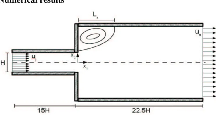
In this section, the multi-field GLS formulation defined by Eqs. (10)-(18) is used to approximate Bingham-Papanastasiou fluids flowing through a sudden planar expansion, as sketched in Fig. 2. The flow domain is described using a Cartesian system in terms of axial x1 and transversal x2 coordinates, with the origin on the centerline of expansion plane. Besides that, taking advantage of the geometry symmetry, only half the channel is simulated. In all computations, the channel aspect ratio is fixed as one-to-four and the lengths of both channels are sufficiently large to avoid entry flow effects – with H = 1 m. In addition, the symbol Lr defines the reattachment length.
A grid independence procedure is performed comparing both the Euler pressure coefficient (
(
)
20
2 /
p i
C = p−p ρu ), with standing
for a reference pressure at the channel outlet and
u
0p
i for the inlet velocity, and the dimensionless shear stress (τ τ τ*= / 0). Three different meshes are considered: (i) M1 with 10,550 Lagrangian bi-linear finite elements; (ii) M2 with 19,800 elements and (iii) M3 with 20,920 elements – for the details of this procedure see Fig. 3, which is subjected to relative errors for the shear stress from 0.09% to 2.84% and for the Euler coefficient from 0.09% to 2.76%. Figure 4 shows details in the expansion vicinity of the selected mesh (M2) with 19,800 elements and 121,686 degrees-of-freedom.
(a)
(b)
(c)
(d) Figure 3. Mesh independence procedure for Re = 0 and Bn = 20 – full view of: (a) Cp and (b) τ
*
; blow-up view of: (c) Cp and (d) τ *
.
As usual in internal flows, no-slip and impermeability boundary conditions are imposed on channel walls, symmetry conditions
2 1 2 12 0
xu u τ
Figure 4. Flow through a 1:4 sudden expansion: detail of the employed finite element mesh at the expansion vicinity.
In order to obtain the dimensionless groups that govern the viscoplastic fluid flow, Eq. (7) may be written in a non-dimension form scaling all Cartesian coordinates by H, all velocities by ui, the pressure by 2
i u
ρ and the shear stress by the material yield stress τ0.
Applying such dimensionless quantities to Eq. (7), one obtains that the governing dimensionless groups for such a flow are the Bingham and Reynolds numbers:
0
Bn p i
H u τ η
=
(21)
Re i
p u H ρ
η
=
(22)
(a)
(b)
(c)
(d)
(e)
(f)
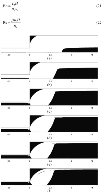
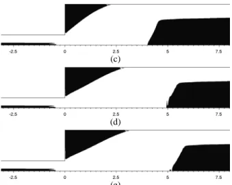
Figure 5. Yielded and unyielded regions for Re=0: (a) Bn = 0.2; (b) Bn = 2; (c) Bn = 20; (d) Bn = 30; (e) Bn = 60; (f) Bn = 100.
The yield stress effect and the inertia effect are taken into account respectively by the Bingham (Eq. (21)) and the Reynolds (Eq. (22)) numbers. The former expressing the relationship between the yield and shear stresses and the latter denoting the relationship between inertia and viscous forces acting on the fluid flow.
Figure 5 investigates the yield stress limit influence on the morphology of yielded (white zones in the pictures, in which
0
* /
τ τ τ= >1) and unyielded (black ones, in which * 1τ < ) material regions, for creeping flows. As Bingham number increases, both the unmoving and moving unyielded zones monotonically increase too – see Figs. 5(a)-5(f). The morphology of yielded and unyielded regions in Bingham flows is related to the yield stress of the material – namely the higher the yield limit is, the greater the unyielded regions are; or, in other words, the easier for the condition
* 1
τ < to occur throughout the flow. Some comments ought to be added to this overall rule. First, for the lowest viscoplastic flow (Bn = 0.2, Fig. 5(a)), while the moving unyielded regions (hereafter, called plug-flows) in the smaller channel are still incipient, the larger channel already presents well-developed plug-flows around the channel centerline and unmoving unyielded regions (hereafter, called dead zones) at the expansion corner. This behavior may be credited to a combination of two factors, namely the higher local shear-rate experimented in the smaller channel and the low yield limit of the flow, Bn = 0.2. These two factors combined generate very low local Bingham numbers along the smaller channel. Next, the monotonic growth of unyielded regions with the increasing of Bingham number seems to be damped when Bingham reaches the value 20 (Fig. 5(c)), after which both the plug-flow and dead zone in the larger channel are almost insensitive to the Bingham increase. Note that the same does not apply to plug-flows in the smaller channel, which still experiment some enlargement even for the highest viscoplastic flows (see Fig. 5(e) and Fig. 5(f)). In addition, it is worth pointing out that plug-flow distance from the expansion plane, in the larger channel, decreases with Bingham increase only for Bingham values less than 20 (Fig. 5(c)). Thereafter, it seems to be almost insensitive to the Bingham growth (Figs. 5(d)-5(f)) – for the same reasons already reported in the comments on the morphology of these regions.
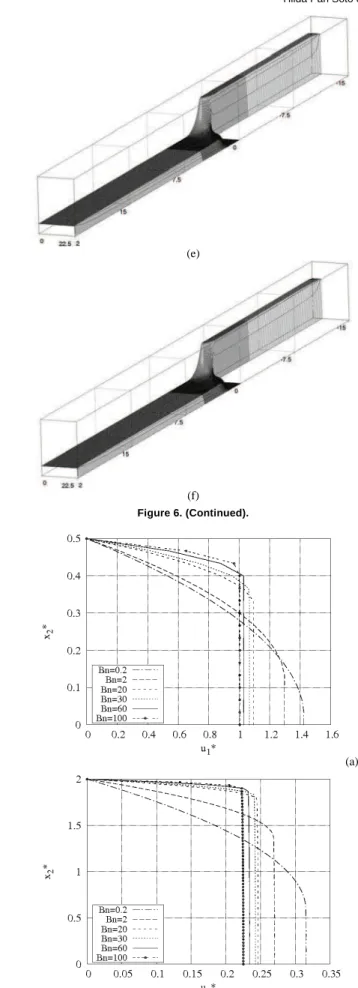
Figure 6 presents elevation plots for the dimensionless axial velocity ( ) through the expansion channel, for creeping flow and Bn = 0.2-100. These figures confirm the foregoing comments introduced in the previous paragraph. In all figures, the plug flows in both channels and the dead zones at the expansion corner are clearly illustrated and complement the behavior described in Fig. 5 – namely, the increasing of unyielded regions with the Bingham number growth. Two points may still be added. The first one, the good insight provided by these elevation plots that permits a clear visualization of the velocity development in viscoplastic fluid flows permitting the identification of the following features of velocity field: (i) for the lowest viscoplastic flows (Figs. 6(a)-6(b)), the entrance length in the smaller channel, imposed by the flat velocity profile at the inlet and its subsequent development into fully-developed viscoplastic profiles; (ii) the plug-flows smoothness and their sharp edges for high viscoplastic situations (Figs. 6(c)-6(f)); and (iii) the strong decay experimented by the maximum velocity in the larger channel thanks to the flow mass conservation. Another point worth mentioning is that Fig. 6 makes clear the narrowness of yielded regions for the most viscoplastic cases (for Bn = 60, Fig. 6(e), and Bn = 100, Fig. 6(f)) – characterizing very thin boundary layers near the channel wall. From the numerical point of view, this issue results in very stiff computational simulations for high Bingham flows, for which only a numerical method containing a proper stabilized strategy might be successful.
(a)
(b)
(c)
(d)
Figure 6. Elevation plots for dimensionless axial velocity along the channel, for Re = 0: (a) Bn = 0.2; (b) Bn = 2; (c) Bn = 20; (d) Bn = 30; (e) Bn = 60; (f) Bn = 100.
(e)
(f)
Figure 6. (Continued).
(a)
(b)
Figure 7 quantitatively investigates the plug-flows in two fully-developed viscoplastic regions in both channels. The figures depict transverse profiles of dimensionless axial velocity u1* for creeping
flow, and Bn = 0.2-100 at in the smaller channel
and at in the larger channel – considering
*
1 1/ 1
x =x H= − 0
*
1 10
x = + *
2 2/
x =x H in both figures. The velocity profiles obey the above established rule, as expected: the more viscoplastic the flow is, the flatter the profiles are – from the quasi-parabolic profile, in the smaller channel, for Bn = 0.2 (Fig. 7(a)), up to the plug-flow profile for Bn = 100 (Fig. 7(b)). From the comparison of Figs. 7(a) and 7(b), the influence of the channel height is noticed. Whereas in Fig. 7(a) the maximum velocity in the smaller channel slightly surpasses 1.42, for the larger channel its value decays to approximately 0.33 – a drop of almost 77% with respect to the smaller channel. This behavior may be explained by two distinct arguments. The first one, a classical incompressible Newtonian feature, is related to the velocity decrease caused by the enlargement of the flow area after the expansion. The second argument is originated by the increasing viscoplastic effects as Bingham grows, which give rise to quasi-uniform velocity profiles – except in the thin yielded material regions near the channel wall – hence decreasing even more their maximum velocities.
(a)
(b)
Figure 8. Dimensionless pressure drop through the channel, for Re = 0 and Bn = 0.2-100: (a) longitudinal profile and elevation plots for (b) Bn = 30; (c) Bn = 60; (d) Bn = 100.
(c)
(d)
Figure 8. (Continued).
The influence of Bingham number on the dimensionless pressure drop ( *
(
)
0
2 / 2
p i
p =C = p−p ρu ) along the channel is
shown in Fig. 8 – with *
1 1/
x =x H. In all cases, the greater the Bingham number is, the more the pressure drops – with all flows presenting a steeper slope in the smaller channel. This general behavior for the pressure drop may be understood recollecting that the viscosity regularization proposed by Papanastasiou (1987) substituted the material unyielded regions prescribed by the Bingham model (Eq. (4)) for yielded regions submitted to very high (but finite) viscosity (Eq. (6)). Thus, viscoplastic flows are much more viscous than the quasi-Newtonian case (for Bn = 0.2, in Fig. 8(a)) as Bingham number increases – see also three-dimension illustrations of the pressure surface in Figs. 8(b)-8(d).
(a)
(c)
(d)
(e)
Figure 9. Yielded and unyielded regions for Bn = 2: (a) Re = 0; (b) Re = 15; (c) Re = 30; (d) Re = 45; (e) Re = 50.
Figure 9 analyzes the influence of inertia effects on the morphology of yielded and unyielded material regions, through the plotting of yielded and unyielded material regions for a mild value of the Bingham number (Bn = 2) and Reynolds number ranging from 0 to 50. As illustrated in the figure, two major effects on the morphology of those regions may be noticed. First, the displacement from the expansion plane experienced by downstream plug-flows in the larger channel and, second, the stretching of dead zones at the expansion corner along the flow streamlines. The former issue is due to the enlargement of entry-flow regions in the larger channel with Reynolds number enhancement. These entry regions present greater shear stresses (τ* > 1) than those experienced in downstream regions of pure shear flows, since, besides the shear component τ12*,
they are also submitted to non-null τ11 *
and τ22 *
normal stresses. This comment is well illustrated in Fig. 10, which presents the inertia influence on extra-stress profiles downstream of the expansion plane at channel wall (x2* = 2), for Bn = 2, and Re = 0
(Fig. 10(a)) and Re = 50 (Fig. 10(b)). Although the GNL model is built to describe pure shear flows and, consequently, is not the most appropriate model to describe complex flows with non-zero normal stress, the morphology of dead zones at the expansion corner may be better understood from these figures. First, note that the end of dead zones corresponds to the intersection between the curves of τ* and τ0
*
in both figures, i.e., the intersection point τ* = 1. Thus, with the increasing of the Reynolds number, this point moves away from the expansion plane – for Re = 0 (from Fig. 10(a) and Fig. 9(a)) its location is at x1 *≃1.25 and, for Re = 50 (from Fig. 10(b) and Fig.
9(e)), it is at x1* 3. ≃
(a)
(b) Figure 10. Extra-stresses longitudinal profiles at x2
*
= 2, downstream of expansion plane, for Bn = 2: (a) Re = 0; (b) Re = 50.
(a)
(b) Figure 11. Extra-stresses longitudinal profiles at x2
*
= 0, downstream of expansion plane, for Bn = 2: (a) Re = 0; (b) Re = 50.
In Fig. 12, inertia and yield stress influence on the vortex length at expansion corner is shown. This figure presents the plotting of the dimensionless reattachment length ( *
/ r r
for an illustration of flow streamlines of the recirculation region at the expansion corner, for Re = 50 and Bn = 0.2-5.0. In addition, a comparison for the Newtonian case (the point Bn = 0 in the curve of Fig. 12(b)) is undertaken against the results of Dagtekin and Ünsal (2010). Both articles present a good adhesion: the latter work yields a value Lr = 8.785 and the current work yields Lr = 8.6.
(a)
(b)
Figure 12. Reattachment Lengths versus: (a) Reynolds numbers, for Bn = 0 and (b) Bingham numbers, for Re = 50.
(a)
(b)
(c)
(d)
(e)
(f)
Figure 13. Flow streamlines for Re = 50: (a) Bn = 0; (b) Bn = 0.2; (c) Bn = 1; (d) Bn = 2; (e) Bn = 3; (f) Bn = 5.
Final conclusions
In this article, a multi-field Galerkin least-squares method in terms of extra-stress, velocity and pressure is employed to approximate inertial flows of Bingham-Papanastasiou fluids through a one-to-four sudden planar expansion. This formulation does not need to satisfy the compatibility conditions involving both pressure-velocity and stress-pressure-velocity finite element sub-spaces and is able to remain stable in high Bingham and Reynolds fluid flows. The inertia and yield stress influence on the morphology of material yield surfaces are evaluated ranging Bingham and Reynolds numbers, respectively. For creeping flows, the more the Bingham number increases, the more the moving and unmoving unyielded material regions monotonically increase too. As a consequence of the unyielded region growth, the flow is subjected to higher pressure drops as Bingham increases. When inertia is taken into account, the Reynolds number increase drives plug-flow zones away from the expansion plane and dead zones at expansion corner are stretched along the main flow streamlines. Furthermore, the reattachment length in the larger channel is severely restrained by the Bingham increase. The numerical results are confirmed with the related literature and ensure the good stability features of the multi-field GLS method employed.
Acknowledgements
The author C. Fonseca thanks CAPES for his graduate scholarship, and authors S. Frey and M. L. Martins-Costa acknowledge CNPq and FAPERJ, for financial support.
References
Abdali, S.S., Mitsoulis, E., Markatos, N.C., 1992, “Entry and exit flows of Bingham fluids”, J. Rheology, Vol. 36, pp. 389-407.
Alexandrou, A.N., Duc, E., Entov, V., 2001 “Inertial, viscous and yield stress effects in Bingham fluid filling of a 2-D cavity”, J. Non-Newtonian
Fluid Mech., Vol. 96, pp. 383-403.
Araujo, J.H.C., Ruas, V., 1998, “A stable finite element method for the axisymmetric three-field Stokes system”, Computer Methods Appl. Mech.
Engng., Vol. 164, pp. 267-286.
Behr, M.A., Franca, L.P., Tezduyar, T.E., 1993, “Stabilized Finite Element Methods for the Velocity-Pressure-Stress Formulation of Incompressible Flows”, Computer Methods Appl. Mech. Engng., Vol. 104, pp. 31-48.
Bird, R.B., Armstrong, R.C., Hassager, O., 1987, “Dynamics of Polymeric Liquids”, Vol. 1: Fluid Mechanics”, 2nd ed., John Wiley & Sons, U.S.A.
Bonvin, J., Picasso, M., Stenberg, R., 2001, “GLS and EVSS methods for a three-field Stokes problem arising from viscoelastic flows”, Computer
Methods Appl. Mech. Engng., Vol. 190, pp. 3893-3914.
Ciarlet, P.G., 1978, “The Finite Element Method for Elliptic Problems”. North Holland, Amsterdam.
Crochet, M.J., Keunings, R., 1982, “Finite element analysis of die swell of a highly elastic fluid”, J. Non-Newtonian Fluid Mech., Vol. 10, pp. 339-356.
Dagtekin, I, Ünnsal, M. 2010, “Numerical analysis of axisymmetric and planar sudden expansion flows for laminar regime”, Int. J. Numer. Meth.
Fluids, DOI: 10.1002/fld.2239.
Fortin, M., Pierre, R., 1989, “On the convergence of the mixed method of Crochet and Marchal for viscoelastic flows”, Comput. Methods Appl.
Mech. Engrg., Vol. 73, pp. 341-350.
Franca, L.P., Frey, S., Hughes, T.J.R., 1992, “Stabilized finite element methods: I. Application to the advective-diffusive model”, Comput. Methods
Appl. Mech. Engrg., Vol. 95, pp. 253-276.
Franca, L.P., Frey, S., 1992, “Stabilized finite element methods: II. The incompressible Navier-Stokes equations”, Comput. Methods Appl. Mech.
Engrg., Vol. 99, pp. 209-233.
Franca, L.P., Stenberg, R., 1991, “Error Analysis of Some Galerkin Least Squares Methods for the Elasticity Equations”, SIAM J. Numer. Anal., Vol. 28/6, pp. 1680-1697.
Hughes, T.J.R., França, L., Balestra, M., 1986, “A New Finite Element Formulation for Computational Fluid Dynamics: V. Circumventing the Babuska-Brezzi Condition: A Stable Petrov-Galerkin Formulation of the Stokes Problem Accommodating Equal-Order Interpolations”, Computer
Methods Appl. Mech. Engrg., Vol. 59, pp. 85-99.
Liu, B.T., Muller, S.J., Denn, M.M., 2002, “Convergence of regularization method for creeping flow of a Bingham material about a rigid sphere”, J. Non-Newtonian Fluid Mech., Vol. 102, pp. 179-191.
Marchal, J.M., Crochet, M.J., 1986, “Hermitian Finite Elements for Calculating Viscoelastic Flow”, J. Non-Newtonian Fluid Mech., Vol. 20, pp. 187-207.
Marchal, J.M., Crochet, M.J., 1987, “A new mixed finite element for calculating viscoelastic flow”, J. Non-Newtonian Fluid Mech., Vol. 26, pp. 77-114.
Mitsoulis, E., Huilgol, R.R, 2004, “Entry flows of Bingham plastics in expansions”, J. Non-Newtonian Fluid Mech., Vol. 122, pp. 45-54.
Papanastasiou, T.C., 1987, “Flows of Materials with Yield”, J. Rheology, Vol. 31, pp. 385-404.
Peric, D., Slijepcevic, S., 2001, “Computational modelling of viscoplastic fluids based on a stabilised finite element method”, Engineering
Computations, Vol. 18, (3/4), pp. 577-591.
Rektorys, K., 1975, “Variational Methods in Mathematics, Science and Engineering”, Reidel, U.S.A.
Rocha. G.N., Poole, R.J., Oliveira, P.J., 2007, “Bifurcation phenomena in viscoelastic flows through a symmetric 1:4 expansion”, J. Non-Newtonian
Fluid Mech., Vol. 141, pp. 1-17.
Roquet, N., Saramito, P., 2008, “An adaptive finite element method for viscoplastic flows in a square pipe with stick-slip at the wall”, J.
Non-Newtonian Fluid Mech., Vol. 155, pp. 101-115.
Singh, J.P., Denn, M.M., 2008, “Interacting two-dimensional bubbles and droplets in a yield-stress fluid”, Physics of Fluids, Vol. 20, pp. 040901-1- 040901-11.
Zinani, F., Frey, S., 2008, “Galerkin Least-Squares Multi-Field Approximations for Flows of Inelastic Non-Newtonian Fluids”, J. Fluids
Engineering, Vol. 130, pp. 081507/1-14.