Carlos Breviglieri
[email protected] Instituto Tecnológico de Aeronáutica CTA/ITA/IEC São José dos Campos 12228-900 SP, BrazilJoão Luiz F. Azevedo
[email protected] Instituto de Aeronáutica e Espaço CTA/IAE/ALA São José dos Campos 12228-903 SP, BrazilEdson Basso
[email protected] Instituto de Aeronáutica e Espaço CTA/IAE/ALA São José dos Campos 12228-903 SP, BrazilAn Unstructured Grid Implementation
of High-Order Spectral Finite Volume
Schemes
The present work implements the spectral finite volume scheme in a cell centered finite volume context for unstructured meshes. The 2-D Euler equations are considered to rep-resent the flows of interest. The spatial discretization scheme is developed to achieve high resolution and computational efficiency for flow problems governed by hyperbolic conser-vation laws, including flow discontinuities. Such discontinuities are mainly shock waves in the aerodynamic studies of interest in the present paper. The entire reconstruction pro-cess is described in detail for the 2ndto 4thorder schemes. Roe’s flux difference splitting method is used as the numerical Riemann solver. Several applications are performed in order to assess the method capability compared to data available in the literature. The results obtained with the present method are also compared to those of essentially non-oscillatory and weighted essentially non-non-oscillatory high-order schemes. There is a good agreement with the comparison data and efficiency improvements have been observed.
Keywords: spectral finite volume, high-order discretization, 2-D euler equations, un-structured meshes
Introduction
Over the past several years, the Computational Aerodynamics Laboratory of Instituto de Aeronáutica e Espaço (IAE) has been developing CFD solvers for two and three dimensional systems (Scalabrin, 2002, Basso, Antunes, and Azevedo, 2003). One re-search area of the development effort is aimed at the implementation of high-order methods suitable for problems of interest to the Insti-tute, i.e., external high-speed aerodynamics. Some upwind schemes such as the van Leer flux vector splitting scheme (van Leer, 1982), the Liou AUSM+flux vector splitting scheme (Liou, 1996) and the Roe flux difference splitting scheme (Roe, 1981) were implemented and tested for second-order accuracy with a MUSCL reconstruction (Anderson, Thomas, and van Leer, 1986). However, the nominally second-order schemes presented results with an order of accuracy smaller than the expected in the solutions for unstructured grids. Aside from this fact, it is well known that total variation diminishing (TVD) schemes have their order of accuracy reduced to first order in the presence of shocks due to the effect of limiters.
This observation has motivated the group to study and to im-plement essentially non-oscillatory (ENO) and weighted essentially non-oscillatory (WENO) schemes in the past (Wolf and Azevedo, 2006).However as the intrinsic reconstruction model of these schemes relies on gathering neighboring cells for polynomial recon-structions for each cell at each time step, both were found to be very demanding on computer resources for resolution orders greater than three, in 2-D, or anything greater than 2ndorder, in 3-D. This fact motivated the consideration of the spectral finite volume method, as proposed by Wang and co-workers (Wang, 2002, Wang and Liu, 2002, 2004, Wang, Liu, and Zhang, 2004, Liu, Vinokur, and Wang, 2006, Sun, Wang, and Liu, 2006), as a more efficient alternative. Such method is expected to perform better than ENO and WENO
Paper accepted August, 2010. Technical Editor: Eduardo Morgado Belo
schemes, compared to the overall cost of the simulation, since it dif-fers on the reconstruction model applied and it is currently extended up to 4th-order accuracy in the present work.
The SFV method is a numerical scheme developed recently for hyperbolic conservation laws on unstructured meshes. The method derives from the Godunov finite volume scheme which has become the state of the art for numerical solutions of hyperbolic conserva-tion laws. It was developed as an alternative tok-exact high-order schemes and discontinuous Galerkin methods (Cockburn and Shu, 1989) and its purpose is to allow the implementation of a simpler and more efficient scheme. The discontinuous Galerkin and SFV methods share some similarities in the sense that both use the same piecewise discontinuous polynomials and Riemann solvers at ele-ment boundaries to provide solution coupling and numerical dissi-pation for stability. Both methods are conservative at element level and suitable for problems with discontinuities. The methods differ on how the necessary variables for polynomial reconstruction are chosen and updated. The SFV method has advantages in this re-construction process. It is compact, extensible and more efficient in terms of memory usage and processing time thank-exact finite volume methods, such as ENO and WENO schemes, since the re-construction stencil is always known and non-singular. This occurs because each element of the mesh, called a Spectral Volume, or SV, is partitioned in a geometrically similar manner into a subset of cells named Control Volumes (CVs). This allows the use of the same polynomial reconstruction for every SV. Afterwards, an approximate Riemann solver is used to compute the fluxes at the SV boundaries, whereas analytical flux formulas are used for flux computation on the boundaries inside the SV. Moreover, each control volume solu-tion is updated independently of the other CVs. The cell averages in these sub-cells are the degrees-of-freedom (DOFs) used to recon-struct a high-order polynomial distribution inside each SV.
two dimensions in a cell centered finite volume context on triangular meshes, with a three-stage TVD Runge-Kutta scheme for time inte-gration. Initially, the paper presents the theoretical formulation of the SFV method for the Euler equations. The reconstruction process of the high-order polynomial is described and some quality aspects of this process are discussed. Afterwards, the flux limiting formula-tion is presented, followed by the numerical results and conclusions.
Nomenclature
c Speed of sound
C Convective operator
e Total energy per unit of volume
E, F Flux vectors in the (x,y) Cartesian directions, respectively
G Gaussian point
h Mesh characteristic size
H Total enthalpy
M Mach number
M∞ Free stream Mach number
~n Unit normal vector to the surface, positive outward
nf Number of faces
p Pressure
Q Vector of conserved properties
S Surface of the control volume
t Time
u, v Velocity components in the (x,y) directions, respectively
z End point of the edge
w Gaussian weight
γ Ratio of specific heats
Γ Edge of the control volume
ρ Density
Subscript
i i-th spectral volume
j j-th control volume
nb nb-th neighbor of the j-th control volume
Superscript n n-th iteration
Theoretical Formulation
Governing Equations
In the present work, the 2-D Euler equations are solved in their integral form as
∂ ∂t Z V QdV + Z V
(∇ ·P~)dV = 0, (1)
whereP~ =Eˆı+Fˆ. The application of the divergence theorem to Eq. (1) yields
∂ ∂t Z V QdV + Z S
(P~·~n)dS= 0. (2)
The vector of conserved variables,Q, and the convective flux vec-tors,EandV, are given by
Q= ρ ρu ρv e
, E=
ρu ρu2+p
ρuv (e+p)u
, F =
ρv ρuv ρv2+p
(e+p)v
. (3)
The system is closed by the equation of state for a perfect gas
p= (γ−1)
e−12ρ(u2+v2)
, (4)
where the ratio of specific heats,γ, is set as1.4for all computations in this work. The flux Jacobian matrix in then=(nx, ny)direction can be written as
B =nx
∂E ∂Q+ny
∂F
∂Q. (5)
The B matrix has four real eigenvalues λ1 = λ2 = vn, λ3 =
vn +c, λ4 = vn −c, and a complete set of right eigenvectors
(r1, r2, r3, r4), wherevn=unx+vnyandcis the speed of sound. LetRbe the matrix composed of these right eigenvectors, then the Jacobian matrix,B, can be diagonalized as
R−1BR= Λ,
(6)
whereΛis the diagonal matrix containing the eigenvalues:
Λ =diag(vn, vn, vn+c, vn−c). (7) In the finite volume context, Eq. (2) can be rewritten for the i-th control volume as
∂Qi
∂t =− 1 Vi
Z
Si
(P~ ·~n)dS, (8)
whereQiis the cell averaged value ofQat timetin thei-th control volume,Vi.
Spatial Discretization
The spatial discretization process determines ak-th order dis-crete approximation to the integral in the right-hand side of Eq. (8). In order to solve it numerically, the computational domain,Ω, with proper initial and boundary conditions, is discretized into N non-overlapping triangles, the spectral volumes (SVs) such that
Ω =
N
[
i=1
Si. (9)
One should observe that the spectral volumes could be composed of any type of polygon, given that it is possible to decompose its bounding edges into a finite number of line segmentsΓK, such that
Si =
[
In the present paper, however, the authors assume that the computa-tional mesh is always composed of triangular elements. Hence, al-though the theoretical formulation is presented for the general case, the actual SV partition schemes are only implemented for triangular grids.
The boundary integral from Eq. (8) can be further discretized into the convective operator form
C(Qi)≡
Z
Si
(P~·~n)dS=
K
X
r=1
Z
Ar
(P~·~n)dS, (11)
whereKis the number of faces ofSiandArrepresents ther−th face of the SV. Given the fact that~nis constant for each line seg-ment, the integration on the right side of Eq. (11) can be performed numerically with ak−thorder accurate Gaussian quadrature for-mula
Z
Ar
(P~·~n)dS=
K X r=1 J X q=1
wrqP(Q(x~ rq, yrq))·~nrAr+O(Arhk). (12)
where(xrq, yrq)andwrqare, respectively, the Gaussian points and the weights on ther-th face ofSiandJ =integer((k+ 1)/2)is the number of quadrature points required on ther−thface. For the second-order schemes, one Gaussian point is used in the integration. Given the coordinates of the end points of the element face,z1and
z2, one can obtain the Gaussian point as the middle point of the
segment connecting the two end points,G1= 12(z1+z2). For this
case, the weight isw1= 1. For the third and fourth order schemes,
two Gaussian points are necessary along each line segment. Their values are given by
G1 =
√
3 + 1
2√3 z1+ (1−
√
3 + 1
2√3 )z2 and (13)
G2 =
√
3 + 1
2√3 z2+ (1−
√
3 + 1 2√3 )z1,
and the respective weights,w1andw2, are set asw1=w2= 12.
Using the method described above, one can compute values of
Qi for instant t for each SV. From these averaged values, recon-struct polynomials that represent the conserved variables,ρ,ρu,ρv
ande; due to the discontinuity of the reconstructed values of the conserved variables over SV boundaries, one must use a numerical flux function to approximate the flux values on the cell boundaries.
The above procedures follow exactly the standard finite volume method. For a given order of spatial accuracy,k, for Eq. (11), using the SFV method, eachSielement must have at least
m=k(k+ 1)
2 (14)
degrees of freedom (DOFs). This corresponds to the number of con-trol volumes thatSishall be partitioned into. If one denotes byCi,j thej-th control volume ofSi, the cell-averaged conservative vari-able,Q, at timet, forCi,jis computed as
qi,j(t) =
1 Vi,j
Z
Ci,j
q(x, y, t)dxdy, (15)
whereVi,jis the volume, or area in the 2-D case, ofCi,j. Once the cell-averaged conservative variables, or DOFs, are available for all
CV swithinSi, a polynomial,pi(x, y)∈Pk−1, with degreek−1, can be reconstructed to approximate theq(x, y)function insideSi, i.e.,
pi(x, y) =q(x, y) +O(hk−1),(x, y)∈Si, (16) wherehrepresents the maximum edge length of allCV swithinSi. The polynomial reconstruction process is discussed in details in the following section. For now, it is enough to say that this high-order reconstruction is used to update the cell-averaged state variables at the next time step for all theCV swithin the computational domain. Note that this polynomial approximation is valid withinSiand some numerical flux coupling is necessary across SV boundaries.
Integrating Eq. (8) inCi,j, one can obtain the integral form for the CV averaged mean state variable
dqi,j dt + 1 Vi,j K X r=1 Z Ar
(f·~n)dS= 0, (17)
wheref represents theE andF fluxes, Kis the number of faces ofCi,jandArrepresents ther−thface of the CV. The numerical integration can be performed with ak−thorder accurate Gaussian quadrature formulation, similarly to the one for the SV elements in Eq. (12).
As stated previously, the flux integration across SV boundaries involves two discontinuous states, to the left and to the right of the face. This flux computation can be carried out using an exact or approximate Riemann solver, or a flux splitting procedure, which can be written in the form
f(q(xrq, yrq))·~nr≈fRiemann(qL(xrq, yrq), qR(xrq, yrq), ~nr), (18)
whereqlis the conservative variable vector obtained by thepi poly-nomial applied at the(xrq, yrq)coordinates andqris the same vec-tor obtained with thepnbpolynomial in the same coordinates of the face. Note that thenbsubscript represents the element to the right of the face, while theisubscript the CV to its left. As the numerical flux integration in the present paper is based on one of the forms of a Riemann solver, this is the mechanism which introduces the upwind and artificial dissipation effects into the method, making it stable and accurate. In this work, the authors have used the Roe flux difference splitting method (Roe, 1981) to compute the numerical flux, i.e.,
fRiemann=froe(qL, qR, ~n)
=1 2
f(qL) +f(qR)−
B
(qR−qL)
, (19)
whereB
is Roe’s dissipation matrix computed from B =R Λ
R−1. (20)
Here,Λ
is the diagonal matrix composed of the absolute values of
Finally, one ends up with the semi-discrete SFV scheme for up-dating the DOFs at control volumes, which can be written as
dqi,j
dt =− 1 Vi,j K X r=1 J X q=1
[wrq·
·fRiemann(Ql(xrq, yrq), Qr(xrq, yrq), ~nr)Ar] (21) where the right hand side of Eq. (21) is the equivalent convective operator,C(qi,j), for thej-th control volume ofSi. It is worth men-tioning that some faces of the CVs, resulting from the partition of the SVs, lie inside the SV element in the region where the polynomial is continuous. For such faces, there is no need to compute the numer-ical flux as described above. Instead, one uses analytnumer-ical formulas for the flux computation, i.e., without numerical dissipation.
Temporal Discretization
The temporal discretization is concerned with solving a system of ordinary differential equations. In the present work, the authors use a third-order, TVD Runge-Kutta scheme (Shu, 1987). Rewriting Eq. (21) in a concise ODE form, one obtains
dq dt =−
1 Vi,j
C(q). (22)
where q=
q1,1
· · · qi,j · · · qN,m
, C(q) =
C(q1,1)
· · ·
C(qi,j) · · ·
C(qN,m)
, (23) and
C(qi,j) =−
1 Vi,j K X r=1 J X q=1 [wrq·
·fRoe(qL(xrq, yrq), qR(xrq, yrq), ~nr)Ar]. (24) Hence, the time marching scheme can be written as
q(1) = qn+ ∆tC(qn),
q(2) = α1qn+α2
h
q(1)+ ∆tC(q(1))i ,
q(n+1) = α3qn+α4
h
q(2)+ ∆tC(q(2))i ,
where thenandn+ 1superscripts denote, respectively, the values of the properties at the beginning and at the end of then-th time step. Theαcoefficients areα1 = 3/4,α2 = 1/4,α3 = 1/3and
α4= 2/3.
Spectral Finite Volume Reconstruction
General Formulation
The evaluation of the conserved variables at the quadrature points is necessary in order to perform the flux integration over the
mesh element faces. These evaluations can be achieved by recon-structing conserved variables in terms of some base functions using the DOFs within a SV. The present work has carried out such recon-structions using polynomial base functions, although one can choose any linearly independent set of functions. LetPmdenote the space ofm-th degree polynomials in two dimensions. Then, the minimum dimension of the approximation space that allowsPmto be complete is
Nm=
(m+ 1)(m+ 2)
2 . (25)
In order to reconstructqinPm, it is necessary to partition the SV intoNmnon-overlapping CVs, such that
Si = Nm
[
j=1
Ci,j. (26)
The reconstruction problem, for a given continuous function inSi and a suitable partition, can be stated as findingpm∈Pmsuch that
Z
Ci,j
pm(x, y)dS=
Z
Ci,j
q(x, y)dS. (27)
With a complete polynomial basis, el(x, y)∈Pm, it is possible to satisfy Eq. (27). Hence,pmcan be expressed as
pm= Nm
X
l=1
alel(x, y), (28)
whereeis the base function vector,[e1,· · · , eN], andais the recon-struction coefficient vector,[a1,· · · , aN]T. The substitution of Eq. (28) into Eq. (27) yields
1 Vi,j Nm X l=1 al Z Ci,j
el(x, y)dS=qi,j. (29)
Ifqdenotes the[qi,1,· · ·, qi,N m]T column vector, Eq. (29) can be rewritten in matrix form as
Sa=q, (30)
where theSreconstruction matrix is given by
S=
1
Vi,1
R
Ci,1e1(x, y)dS · · ·
1
Vi,1
R
Ci,1eN(x, y)dS
..
. · · · ...
1
Vi,N
R
Ci,N e1(x, y)dS · · ·
1
Vi,N
R
Ci,NeN(x, y)dS
(31)
and, then, the reconstruction coefficients,a, can be obtained as
a=S−1q,
(32)
provided that S is non-singular. Substituting Eq. (32) into Eq. (27), pm is, then, expressed in terms of shape functions L =
[L1,· · · , LN], defined asL=eS−1, such that one could write
pm= Nm
X
j=1
Table 1. Polynomial base functions.
reconstruction order e
linear [ 1x y]
quadratic [ 1x y x2xy y2]
cubic [ 1x y x2xy y2x3x2y xy2y3]
Equation (33) gives the value of the conserved state variable,q, at any point within the SV and its boundaries, including the quadrature points,(xrq, yrq). The above equation can be interpreted as an inter-polation of a property at a point using a set of cell averaged values, and the respective weights which are set equal to the corresponding cardinal base value evaluated at that point.
Once the polynomial base functions,el, are chosen, theLshape functions are uniquely defined by the partition of the spectral vol-ume. The shape and partition of the SV can be arbitrary, as long as theS matrix is non-singular. The major advantage of the SFV method is that the reconstruction process does not need to be carried out for every mesh elementSi. Once the SV partition is defined, the same partition can be applied to all mesh elements and it results in the same reconstruction matrix. That is, the shape functions at cor-responding flux integration points over different SVs have the same values. One can compute these coefficients as a pre-processing step and they do not change along the simulation. This single reconstruc-tion is carried out only once for a standard element, for instance an equilateral triangle, and it can be read by the numerical solver as in-put. This is a major difference when compared tok-exact methods such as ENO and WENO schemes, for which every mesh element has a different reconstruction process at every time step. Clearly, the SFV is more efficient in this step. Recently, several partitions for both 2-D and 3-D SFV reconstructions were studied and refined (Wang, Liu, and Zhang, 2004, Chen, 2005). For the present work, the partition schemes are presented in the following sections. More-over, the polynomial base functions for the linear, quadratic and cu-bic reconstructions are listed in Table 1.
Partition Quality
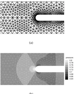
There are many possible different partition schemes for the SFV method reconstructions. The problem is to find one that produces the smoother interpolation of the conserved variables, so that it im-proves the method’s convergence and stability aspects. Until re-cently a parameter named Lebesque constant (Chen and Babuska, 1995) was computed for a given partition and its quality or smooth-ness was determined by its value. The lower this value the better the partition. More detailed description of this parameter can be found in (Wang, 2002, Wang and Liu, 2004, Wang, Liu, and Zhang, 2004). The linear partition is defined in the following section and it can be easily defined. For the quadratic partition, the authors have first used the one presented by Sun and co-workers (Sun, Wang, and Liu, 2006) as shown in Fig. 1 named SV3W in this work. It was tested with different simulations and yielded good results. To verify its convergence aspect we tried a simple test. A blunt body with zero angle of attack withM∞= 0.4was simulated with a mesh of 1014
Figure 1. SV3W quadratic partition.
triangles and CF L = 0.3, as shown in Fig. 2(a). This partition scheme was able to reach machine zero and a solution, but it was noted an instability during the convergence history as shown in Fig. 3. Once the density residual dropped close to -10 it begun to rise and peaked at -7. We were interested to see if this partition scheme would cause the simulation to diverge and so it was simulated up to 1 million iterations and it reached machine zero and produced the result shown in Fig. 2(b) for pressure distribution. This fact brought to our attention the need to investigate other partitions. Indeed this effect was much more noticeable in the cubic reconstruction. The authors first considered the cubic partition scheme proposed by Sun and co-workers (Sun, Wang, and Liu, 2006), named here partition SV4W, shown in Fig. 4. It was unable to produce results for this test case and diverged the simulation as can be seen in the convergence history, Fig. 5.
The quality of the partition is not totally related to a small value of the Lebesgue constant. There are other parameters that can influence its quality as discussed by van Abeele and Lacor (van den Abeele and Lacor, 2007). They showed that the third and fourth order partition schemes shown above can become unstable for a given mesh,CF Lnumber and simulation parameters. Also, they proposed improved partitions for these schemes, and these are present in the following sections.
Linear Reconstruction
(a)
pressure 0.8 0.78 0.76 0.74 0.72 0.7 0.68 0.66 0.64
(b)
Figure 2. Blunt body test case mesh and pressure distribution.
Figure 3. Convergence history for SV3W partition test on the blunt body test case.
Figure 4. SV4W cubic partition.
Figure 5. Convergence history for SV4W partition test on blunt body test case.
CV mesh. The reader should observe that the authors implemented the SFV method for a cell-centered data structure. The high-order polynomial distribution is used to obtain the properties at the ghost boundary face where the desired boundary conditions are imposed.
The code has an edge-based data structure such that it computes the convective operator for the faces instead of computing it for the volume. This approach saves a significant amount of time over tra-ditional implementations. For each CV element face, a database is created relating the face start and end node indices, its neighbors (left and right), whether it is an internal or external face, that is, if it lies inside a given SV or on its boundaries, and how many quadrature points it has. This information,edgecv ={n1, n2, i, nb, type, qdr},
is obtained once connectivity and neighboring information is avail-able. The linear partition is presented in Fig. 7. It yields a total of 7 points, 9 faces (6 are external faces and 3 internal ones), 9 quadrature points and it has a Lebesgue constant value of 2.866. The linear polynomial for the SFV method depends only on the base functions and the partition shape. The integrals of the reconstruc-tion matrix in Eq. (31) are obtained analytically (Liu and Vinokur, 1998) for fundamental shapes. The shape functions, in the sense of Eq. (33), are calculated and stored in memory for the quadrature points, (xrq, yrq), of the standard element. Such shape functions have the exact same value for the quadratures points of any other SV of the mesh, provided they all have the same partition. There is one quadrature point located at the middle of every CV face.
Quadratic Reconstruction
Table 2. Linear partition: barycentric coordinate of the vertices.
node index node 1 node 2 node 3
1 1 0 0
2 1/2 1/2 0
3 0 1 0
4 0 1/2 1/2
5 0 0 1
6 1/2 0 1/2
7 1/3 1/3 1/3
Table 3. Linear partition: control volumes connectivity.
CV nf n1 n2 n3 n4
1 4 6 1 2 7
2 4 2 3 4 7
3 4 4 5 6 7
Figure 6. Standard spectral element.
Figure 7. Linear partition for the SFV method.
Table 4. Quadratic partition: barycentric coordinate of the vertices.
node index node 1 node 2 node 3
1 1 0 0
2 0.909 0.091 0
3 0.091 0.909 0
4 0 1 0
5 0 0.909 0.091
6 0 0.091 0.909
7 0 0 1
8 0.091 0 0.909
9 0.909 0 0.091
10 0.820 0.091 0.091
11 0.091 0.820 0.091
12 1/3 1/3 1/3
13 0.091 0.091 0.820
Table 5. Quadratic partition: control volumes connectivity.
CV nf n1 n2 n3 n4 n5
1 4 1 2 10 9
-2 4 3 4 5 11
-3 4 6 7 8 13
-4 5 2 3 11 12 10
5 5 5 6 13 12 11
6 5 8 9 10 12 13
connectivity table. The ghost creation process and edge-based data structure are the same as for the linear reconstruction case. The par-tition used in this work is the one proposed by van Abeele and Lacor (van den Abeele and Lacor, 2007) named SV3A here, shown in Fig. 8. It has a total of 13 points, 18 faces (9 external faces and 9 internal ones), 36 quadrature points and it has a Lebesgue constant value of 3.075. The shape functions, in the sense of Eq. (33), are obtained as in the linear partition. The reader should note that, in this case, the base functions have six terms that shall be integrated. Again, these terms are exactly obtained (Liu and Vinokur, 1998) and kept in memory.
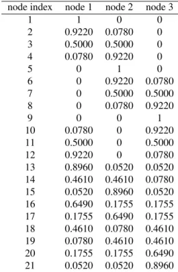
Table 6. Cubic partition: barycentric coordinate of the vertices.
node index node 1 node 2 node 3
1 1 0 0
2 0.9220 0.0780 0
3 0.5000 0.5000 0
4 0.0780 0.9220 0
5 0 1 0
6 0 0.9220 0.0780
7 0 0.5000 0.5000
8 0 0.0780 0.9220
9 0 0 1
10 0.0780 0 0.9220
11 0.5000 0 0.5000
12 0.9220 0 0.0780
13 0.8960 0.0520 0.0520 14 0.4610 0.4610 0.0780 15 0.0520 0.8960 0.0520 16 0.6490 0.1755 0.1755 17 0.1755 0.6490 0.1755 18 0.4610 0.0780 0.4610 19 0.0780 0.4610 0.4610 20 0.1755 0.1755 0.6490 21 0.0520 0.0520 0.8960
Cubic Reconstruction
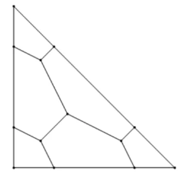
For the cubic reconstruction,m = 3, one needs to partition the SV in ten sub-elements and to use the base vector as defined in Table 1. The barycentric coordinates are given in Table 6 follow-ing the node orientation in Fig. 6. The connectivity information of the CVs is given in Table 7. The ghost creation process and edge-based data structure is the same as for the linear and quadratic recon-struction cases. As a matter of fact, the same algorithm utilized to perform these tasks can be applied to higher order reconstructions. The partition used in this work is the improved one cubic partition (van den Abeele and Lacor, 2007) named SV4A, presented in Fig. 9 and has a total of 21 points, 30 faces (12 are external faces and 18 are internal ones) 60 quadrature points and it has a Lebesgue con-stant value of 4.2446 against 3.4448 of the SV4W partition. Note that for this case, the smaller Lebesgue constant was not favorable to the scheme. The shape functions, in the sense of Eq. (33), are ob-tained as in the linear partition in a pre-processing step. The simple test case was applied to this partition scheme to check if it indeed was more stable that the SV4W partition. It produced a solution and reached machine zero convergence as can be seen in Fig. 10.
Limiter Formulation
For the Euler equations, it is necessary to limit some recon-structed properties in order to maintain stability and convergence of the simulation if it contains discontinuities. Although the use of the conserved properties would be the natural choice, the litera-ture (van Leer, 1979, Bigarella, 2007) shows that it lacks robustness,
Table 7. Cubic partition: control volumes connectivity.
CV nf n1 n2 n3 n4 n5 n6
1 4 1 2 13 12 -
-2 4 4 5 6 15 -
-3 4 8 9 10 17 -
-4 4 2 3 14 13 -
-5 4 3 4 15 14 -
-6 4 6 7 16 15 -
-7 4 7 8 17 16 -
-8 4 10 11 18 17 -
-9 4 11 12 13 18 -
-10 6 13 14 15 16 17 18
Figure 9. SV4A cubic partition scheme.
since it allows for negative values of pressure in the domain after the limited reconstruction operation. The limiter operator is applied in each component of the primitive variable vector,qp= (ρ, u, v, p)T, derived from the conserved variables of the CV averaged mean and its quadrature points. For each CV, the following numerical mono-tonicity criterion is prescribed:
qpi,jmin≤qi,jp (xrq, yrq)≤qpi,j max
, (34)
whereqpi,jmin andqpmax
i,j are the minimum and maximum cell av-eraged primitive variables among all neighboring CVs that share a face withCi,j, defined as
qpi,jmin= min(qpi,j,min(1≤r≤K)qpi,j,r)
qpi,jmax= max(qpi,j,max(1≤r≤K)qpi,j,r)
(35)
If Eq. (34) is strictly enforced, the method becomes TVD (Leveque, 2002). However, it would become first order accurate and compromise the general accuracy of the solution. To maintain high-order accuracy away from discontinuities, small oscillations are al-lowed in the simulation following the idea of TVB methods (Shu, 1987). If one expresses the reconstruction for the quadrature points, in the sense of Eq. (33) converted to primitive variables, as a differ-ence with respect to the cell averaged mean,
∆qprq=pi(xrq, yrq)−qpi,j, (36) then no limiting is necessary if
|∆qrq| ≤4Mqh2rq, (37)
whereMq is a user chosen parameter. Different Mq values must be used for the different primitive variables which have, in general, very different scales. Then it is scaled according to
Mq =M(qpmax−qpmin), (38)
whereMis the input constant independent of the component,qpmax andqpmin are the maximum and minimum of the CVs-averaged primitive variables over the whole computational domain. Note that ifM = 0, the method becomes TVD. If Eq. (36) is violated for any quadrature point it is assumed that its CV is close to a discontinuity, and the solution is linearly reconstructed:
qi,jp =qpi,j+∇qpi,j·(~r−r~ij), ∀~r∈Ci,j. (39) The solution is assumed linear also for all CVs inside a SV if any of its CVs are limited. Gradients are computed with the aid of the gradient theorem (Swanson and Radespiel, 1991), in which deriva-tives are converted into line integrals over the cell faces. This gradi-ent may not satisfy Eq. (34). Therefore, it is limited by multiplying a scalarφ∈[0,1]such that the limited solution satisfies
qi,jp =qpi,j+φ∇qpi,j·(~r−r~ij). (40) Theφscalar is computed following the general orientation of the literature, such that it satisfies the monotonicity constraint. In this work, thevanAlbadalimiter is used (Hirsch, 1990). The limited properties at the quadrature points are then converted to conserved variables before the numerical flux calculation. After this operation, the properties are no longer continuous within the SV if any of its CVs is limited, thus the numerical flux is used on the internal faces, instead of the analytical flux.
Numerical Results
The results presented here attempt to validate the implementation of the data structure, boundary condition treatment, numerical sta-bility and resolution of the SFV method. First, the simulation of the supersonic wedge flow with an oblique shock wave is carried out, for which the analytical solution is known (Anderson, 1982). Second, the transonic external flow over a NACA 0012 airfoil is considered. Next, the simulation of the Ringleb flow is performed followed by the shock tube problem. These test cases were selected to check upon the method capability to deal with discontinuities with the pro-posed limiter and to measure the effective order of the scheme. For the presented results, density is made dimensionless with respect to the free stream condition and pressure is made dimensionless with respect to the density times the speed of sound squared. For the steady case simulations the CFL number is set as a constant value and the local time step is computed using the local grid spacing and characteristic speeds.
Wedge Flow
The first test case is the computation of the supersonic flow field past a wedge with half-angleθ= 10deg. The computational mesh has 816 nodes and 1504 volumes. For comparison purposes, the sec-ond, third and fourth order SFV methods were utilized along with other schemes. The leading edge of the wedge is located at coordi-natesx= 0.25andy = 0.0. The computational domain is bounded along the bottom by the wedge surface and by an outflow section before the leading edge. The inflow boundary is located at the left and top of the domain, while the outflow boundary is located ahead of the wedge and at the right of the domain. The analytical solution gives the change in properties across the oblique shock as a function of the free stream Mach number and shock angle, which is obtained from theθ−β−M achrelation. For this case, a free stream Mach number of M1 = 5.0 was used, and the oblique shock angleβ is
obtained as ≈ 19.5 deg. For the analytical solution, the pressure ratio isp2/p1 ≈3.083and the Mach number past the shock wave
ofM2 ≈3.939. The numerical solutions of the SFV method are in
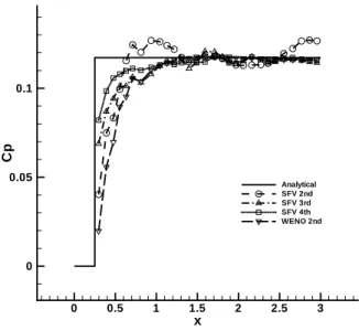
good agreement with the analytical solution. Also, a simulation with the second order WENO (Wolf and Azevedo, 2006) was performed to compare the resolution of the methods, as can be seen in Fig. 11. Note that the SFV scheme is the one that better approximates the jump in pressure on the leading edge. The pressure ratio and Mach number after the shock wave for the fourth order SFV scheme were computed asp2/p1 ≈ 3.047andM2 ≈ 3.901. The pressure
con-tours for this solution can be seen in Fig. 12.
For these simulations the use of the limiter was necessary and the
x
C
p
0 0.5 1 1.5 2 2.5 3
0 0.05 0.1
Analytical SFV 2nd SFV 3rd SFV 4th WENO 2nd
Figure 11. Supersonic wedge flow pressure coefficient distribution for various schemes.
pressure 2 1.8 1.6 1.4 1.2 1 0.8
Figure 12. Supersonic wedge flow pressure contours obtained with fourth order SFV.
scheme reached the same number of iterations after about 100 min-utes. The solution in terms of Cp distribution of both schemes is presented in Fig. 11. This simulation shows the improved efficiency of the SFV method. Both simulations were carried out with an AMD Opteron 246 system running the Linux operational system.
Ringleb Flow
The Ringleb flow simulation consists in an internal subsonic flow which has an analytical solution of the Euler equations derived with the hodograph transformation (Shapiro, 1953). The flow depends on the inverse of the stream functionkand the velocity magnitudeq. In the present computation, we choose the valuesk= 0.4andk= 0.6
to define the boundary walls, andq = 0.35to define the inlet and outlet boundaries. With this parameters, the Ringleb flow represents a subsonic flow around a symmetric blunt obstacle, and is irrota-tional and isentropic. This simulation considered four meshes with
128,512,2048and8192elements. The analytical and numerical solutions were computed in all of these meshes so we could mea-sure how close the numerical results were from the exact ones. This
Figure 13. Supersonic wedge flow limited CVs for pressure, second order SFV.
Figure 14. Supersonic wedge flow limited CVs for pressure, fourth order SFV.
difference was computed using theL2 error norm of the density.
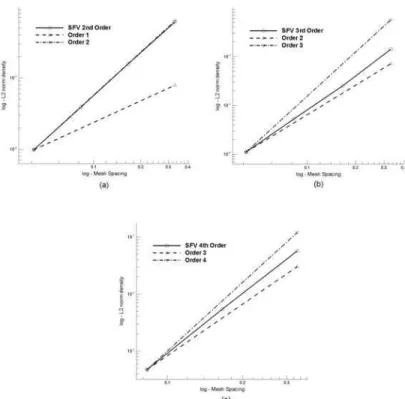
The analytical solution was used as initial condition for all numeric simulations. As the mesh is refined one expects this error to dimin-ish. Analyzing this information on all meshes in a logarithm scale, we can calculate the effective order of the method by computing the slope of the least squares linear fit curve of all meshes errors. This is what is represented in Fig. 16 for the second, third and fourth or-der simulations. The oror-der of the SFV was computed as1.956for second order,2.337for the third order and3.671for the fourth order case. The mesh with2048elements is shown in Fig. 17 along with its analytical and numeric third order density distribution.
A high-order representation of the curved boundaries of the ge-ometry is required to maintain the high resolution of the method (Wang and Liu, 2006, van den Abeele and Lacor, 2007). The high-order boundary representation also reduces the total number of SVs in the mesh. Using standard linear mesh elements one needs so many elements only to represent such curved boundaries. The simulations performed for this case did not consider a curvature approximation of the boundaries and for that reason it is assumed that lower than expected orders were obtained. Note that the measured order of the linear SFV reconstruction is indeed second order accurate, since the representation of the boundary elements as straight lines do not com-promise the order of the method, as shown in Fig. 16(a). The values forkandqparameters of the geometry were chosen so that the flow is subsonic everywhere in the domain in an attempt to reduce the er-rors produced by not using a high-order boundary representation or possible development of a shock wave (Wang and Liu, 2006). Even though, for the fourth order scheme on the finest mesh the simulation actually diverged.
Shock Tube Problem
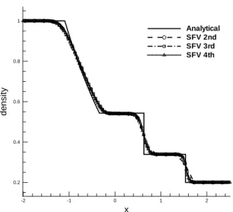
The third test case analyzed is a shock tube problem with length 10 and height 1, in dimensionless units, discretized with a mesh containing 4697 nodes and 8928 triangular control volumes and is shown in Fig. 18. The results presented here are for a pressure ra-tio, p1 = p4 = 5.0. Here, p1 denotes the initial static pressure in the driver section (high-pressure side) of the shock tube, whereas p4 denotes the corresponding initial static pressure in the driven sec-tion (low-pressure side) of the shock tube. It was assumed that both sides of the shock tube were originally at the same temperature. In this problem, a normal shock wave moves from the driver section of the shock tube to the driven section. As the shock wave propagates to the right, it increases the pressure and induces a mass motion of the gas behind it. The interface between the driver and driven gases is represented by a contact discontinuity. An expansion wave propa-gates to the left, smoothly and continuously decreasing the pressure in the driver section of the shock tube. All these physical phenomena are well captured by the SFV schemes.
Figures 19 and 20(a) present the density and pressure distribu-tion for the flow in the shock tube for an instant of time equal to 1.0 dimensionless time units after diaphragm rupture. The results pre-sented were obtained along the shock tube centerline. The results are plotted for the second, third and fourth order SFV scheme. One can see in the density distribution that the results of the schemes are in good agreement with the analytical solution. However, it is
possi-Figure 16. Measured orders with (a) second, (b) third and (c) fourth order SFV method for the Ringleb flow problem.
Figure 18. Mesh considered for the shock tube problem.
x
d
e
n
s
it
y
-2 -1 0 1 2
0.2 0.4 0.6 0.8 1
Analytical SFV 2nd SFV 3rd SFV 4th
Figure 19. Density distribution along the centerline of the shock tube att= 1.
ble to see that the quadratic and cubic reconstructions were limited to the point that most of their CVs were linearly reconstructed. Nev-ertheless, the resolution of these methods for the discontinuities is greater than that of the second order scheme, as noted on the pres-sure distribution at Fig. 20(b).
NACA 0012 Airfoil
For the NACA 0012 airfoil simulation, a mesh with8414 ele-ments and4369nodes was used in the same conditions of the exper-imental data (McDevitt and Okuno, 1985), that is, freestream Mach number value ofM∞ = 0.8and0 deg angle-of-attack. The sec-ond, third and fourth order schemes were computed with aCF L
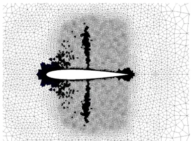
value of 0.5, 0.3 and 0.2, respectively. Figure 21 shows the results of the simulation using the fourth order SFV method. Its agreement with the experimental data, in terms of shock position and pressure coefficient (Cp) values, is very reasonable and the resolution of the shock wave is really sharp, with only one mesh element to represent it. The same is true for the other schemes. Note that the results pre-sented are those for the SV mesh for all cases. For this simulation the use of limiter is also necessary, and the limiter range parameter isM = 50.
The region where the limiter works in the CVs is shown if Fig. 22 for the second order scheme and in Fig. 23 for the third order scheme for pressure. For the linear reconstruction only the CVs close to the shock wave were limited. For the third order scheme, most SVs on the shock wave region were linearly reconstructed and
x
p
re
s
s
u
re
-5 -4 -3 -2 -1 0 1 2 3 4 5
0.2 0.3 0.4 0.5 0.6 0.7 0.8
Analytical SFV 2nd SFV 3rd SFV 4th
(a)
x
p
re
s
s
u
re
0 1 2 3
0.15 0.2 0.25 0.3 0.35
Analytical SFV 2nd SFV 3rd SFV 4th
(b)
pressure
1.05 1 0.95 0.9 0.85 0.8 0.75 0.7 0.65 0.6 0.55 0.5 0.45
Figure 21. Pressure contours on NACA 0012 airfoil, third order SFV scheme.
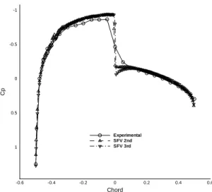
some limited. The choice of an adequate value for theM parameter can lead to a lower usage of the limiter operator. The fourth order SFV scheme achieved very similar results compared to the 3rdorder scheme, given the fact that most CVs on the shock region were lim-ited. The numerical results for the pressure contours are plotted in Fig. 21 for the third-order SFV scheme. Figure 24 indicates that both the second and third order methods capture the shock wave over the airfoil, with a single SV element in it. The Cp distributions in the post-shock region shows that the influence of the limiter operator re-duced the third order scheme resolution. It is important to emphasize that the present computations are performed assuming inviscid flow. Nevertheless, the computational results are in good agreement with the available experimental data. One should observe, however, that the pressure rise across the shock wave, in the experimental results, is spread over a larger region due to the presence of the boundary layer and the consequent shock-boundary layer interaction that nec-essarily occurs in the experiment. For the numerical solution, the shock presents a sharper resolution, as one can expect for an Euler simulation.
Conclusions
The second, third and fourth order spectral finite volume method were successfully implemented and validated for external and in-ternal flow problems, with and without discontinuities. Tests were performed with different partition schemes and it was shown that it can greatly influence the method behavior. The SV partitions in the present work were not the ones with the smallest Lebesgue con-stant, used until recently to indicate the quality of the polynomial interpolation, but those that produced a smoother interpolation.
The effective order of the schemes was measured using the Ringleb flow case and are in the expected values for the current im-plementation. Further modifications in the code that support cur-vature boundaries representation is necessary in order to maintain
Figure 22. Limited CVs for pressure on NACA 0012 airfoil, second order SFV scheme.
Chord
C
p
-0.6 -0.4 -0.2 0 0.2 0.4 0.6
-1
-0.5
0
0.5
1
Experimental SFV 2nd SFV 3rd
Figure 24. Cp distribution for NACA 0012 airfoil for SFV method.
high-order resolution for such simulations. The method behavior for resolution greater than second order showed to be in good agree-ment with both experiagree-mental and analytical data. Furthermore, the results obtained were indicative that the current method can yield so-lutions with similar quality at a much lower computational resource usage than traditionalk−exactschemes, as demonstrated in the su-personic wedge case compared to the WENO fourth order scheme. The method seems suitable for the aerospace applications of interest to IAE in the sense that it is compact, from an implementation point of view, extensible to higher orders, geometry flexible, as it handles unstructured meshes, and computationally efficient.
Acknowledgements
The authors gratefully acknowledge the partial support pro-vided by Conselho Nacional de Desenvolvimento Científico e Tec-nológico, CNPq, under the Integrated Project Research Grant No. 312064/2006-3. The authors are also grateful to Fundação de Am-paro à Pesquisa do Estado de São Paulo, FAPESP, which also partially supported the present research through the Project No. 2004/16064-9.
References
J. D. Anderson. Modern Compressible Flow, with Historical Per-spective - 2nd Edition. McGraw-Hill, Boston, 1982.
W. K. Anderson, J. L. Thomas, and B. van Leer. Comparison of finite volume flux vector splittings for the Euler equations. AIAA Journal, 24(9):1453–1460, 1986.
E. Basso, A. P. Antunes, and J. L. F. Azevedo. Chimera simulations of supersonic flows over a complex satellite launcher
configura-tion. Journal of Spacecraft and Rockets, 40(3):345–355, May-June 2003.
E. D. V. Bigarella. Advanced Turbulence Modelling for Complex Aerospace Applications. Ph.D. Thesis, Instituto Tecnológico de Aeronáutica, São José dos Campos, SP, Brazil, 2007.
Q. Chen and I. Babuska. Approximate optimal points for polyno-mial interpolation of real functions in an interval and in a triangle. Comput. Methods Appl. Mech. Engrg., 128:405–417, 1995.
Q. Y. Chen. “Partitions for Spectral (Finite) Volume Reconstruction in the Tetrahedron,” IMA Preprint Series No. 2035, Minneapolis, MN, April 2005.
B. Cockburn and C. W. Shu. TVB Runge-Kutta local projection dis-continuous Galerkin finite element method for conservation laws II: General framework. Mathematics of Computation, 52:441– 435, 1989.
C. Hirsch. Numerical Computation of Internal and External Flows. Wiley, New York, 1990.
R. J. Leveque. Finite Volume Methods For Hyperbolic Problems. Cambridge University Press, Cambridge, 2002.
M. S. Liou. A sequel to AUSM: AUSM+.Journal of Computational Physics, 129(2):364–382, Dec. 1996.
Y. Liu and M. Vinokur. Exact integrations of polynomials and sym-metric quadrature formulas over arbitrary polyhedral grids. Jour-nal of ComputatioJour-nal Physics, 140(1):122–147, Feb. 1998.
Y. Liu, M. Vinokur, and Z. J. Wang. Spectral (finite) volume method for conservation laws on unstructured grids V: Extension to three-dimensional systems. Journal of Computational Physics, 212(2): 454–472, March 2006.
J. McDevitt and A. F. Okuno. Static and dynamic pressure mea-surements on a NACA 0012 airfoil in the Ames high Reynolds number facility. NASA TP-2485, NASA, Jun. 1985.
P. L. Roe. Approximate Riemann solvers, parameter vectors, and difference schemes. Journal of Computational Physics, 43(2): 357–372, 1981.
L. C. Scalabrin.Numerical Simulation of Three-Dimensional Flows over Aerospace Configurations. Master Thesis, Instituto Tec-nológico de Aeronáutica, São José dos Campos, SP, Brazil, 2002.
A. H. Shapiro.The Dynamics and Thermodynamics of Compressible Fluid Flow. Wiley, New York, 1953.
W. C. Shu. TVB uniformly high-order schemes for conservation laws. Mathematics of Computation, 49:105–121, 1987.
R. C. Swanson and R. Radespiel. Cell centered and cell vertex multi-grid schemes for the Navier-Stokes equations. AIAA Journal, 29 (5):697–703, 1991.
K. van den Abeele and C. Lacor. An accuracy and stability study of the 2D spectral volume method. Journal of Computational Physics, 226(1):1007–1026, Sept. 2007.
B. van Leer. Towards the ultimate conservative difference scheme. V. A second-order sequel to Godunov’s method.Journal of Com-putational Physics, 32(1):101–136, Jul. 1979.
B. van Leer. Flux-vector splitting for the Euler equations. Lecture Notes in Physics, 170:507–512, 1982.
Z. J. Wang. Spectral (finite) volume method for conservation laws on unstructured grids: Basic formulation. Journal of Computational Physics, 178(1):210–251, May 2002.
Z. J. Wang and Y. Liu. Spectral (finite) volume method for conserva-tion laws on unstructured grids II: Extension to two-dimensional scalar equation. Journal of Computational Physics, 179(2):665– 698, Jul. 2002.
Z. J. Wang and Y. Liu. Spectral (finite) volume method for conser-vation laws on unstructured grids III: One-dimensional systems and partition optimization. Journal of Scientific Computing, 20 (1):137–157, Feb. 2004.
Z. J. Wang and Y. Liu. Extension of the spectral volume method to high-order boundary representation. Journal of Computational Physics, 211(1):154–178, Jan. 2006.
Z. J. Wang, Y. Liu, and L. Zhang. Spectral (finite) volume method for conservation laws on unstructured grids IV: Extension to two-dimensional systems. Journal of Computational Physics, 194(2): 716–741, March 2004.
W. R. Wolf and J. L. F. Azevedo. High-order unstructured essentially nonoscillatory and weighted essentially nonoscillatory schemes for aerodynamic flows. AIAA Journal, 44(10):2295–2310, Oct. 2006.