Antonio Marcos G. de Lima
[email protected]Domingos Alves Rade
[email protected] Federal University of Uberlândia School of Mechanical Engineering P.O.Box 593 38400-902 Uberlândia, MG, BrazilNoureddine Bouhaddi
[email protected] University of Franche-Comté FEMTO-ST Applied Mechanics Laboratory 25000 Besançon, FranceOptimization of Viscoelastic Systems
Combining Robust Condensation and
Metamodeling
The effective design of viscoelastic dampers as applied to real-world complex engineering structures can be conveniently carried out by using modern multiobjective numerical optimization techniques. The large number of evaluations of the cost functions normally combined with the typically high dimensions of finite element models of industrial structures makes multiobjective optimization very costly, sometimes unfeasible. Those difficulties motivate the study reported in this paper, in which a strategy is proposed consisting in the use of evolutionary algorithms specially adapted to multiobjective optimization of viscoelastic systems, combined with robust condensation and metamodeling. After the discussion of various theoretical aspects, a numerical application is presented to illustrate the use and demonstrate the effectiveness of the methodology proposed for the optimal design of viscoelastic constrained layers.
Keywords: multiobjective optimization, robust condensation, viscoelastic damping, artificial neural networks, finite elements
Introduction
1Passive control is recognized as being advantageous in terms of stability, effectiveness in broader bandwidths and ease of implementation (Nashif et al., 1985). In particular, the use of viscoelastic materials has been regarded as a convenient strategy in many types of industrial applications, where they can be applied either as discrete devices or surface treatments at a relatively low cost (Samali and Kwok, 1995; Rao, 2001; de Lima et al., 2009; Espíndola et al., 2005). However, viscoelastic materials present some inherent drawbacks such as the influence of operational and environmental factors (frequency, temperature, pre-loads, moisture, etc.). Also, viscoelastic damping systems (specially, surface treatments) are prone to induce considerable mass additions. This last feature leads to the necessity of performing optimization aiming at achieving the desired performance and, at the same time, complying with design and construction constraints.
In the last decades, much effort has been devoted to the development of finite element (FE) models capable of accounting for the typical dependence of the viscoelastic behavior with respect to frequency and temperature (Bagley and Torvik, 1983; MacTavish and Hughes, 1993; Lesieutre and Lee, 1996; Galucio et al., 2004). As a result, it is currently possible to model complex real-world engineering structures such as automobiles, airplanes, communication satellites, buildings and space structures (Balmès and Germès, 2002). A natural extension of this modeling capability is the optimization of the viscoelastic devices aiming the reduction of cost and/or the maximization of performance (Hao et al., 2004; Lee et al., 2004). In the quest for optimization, engineers are frequently faced with conflicting objectives. Such situations are conveniently dealt with by the so-called multiobjective or multicriteria optimization approach (Eschenauer et al., 1990). However, multiobjective optimization generally requires a large number of evaluations of the cost functions involved. For large finite element models of viscoelastic systems, typically composed of many thousands of degrees-of-freedom (DOFs), if such evaluations are made based on exact response computations performed on the full FE matrices, computation times can become prohibitive.
The work reported herein intends to propose a general strategy for the reduction of the computational burden involved in the optimization of viscoelastic structures by combining Multiobjective Evolutionary Algorithms (MOEAs), robust condensation and Artificial Neural Networks (ANNs). The motivation for the use of
Paper accepted June, 2010. Technical Editor: Paulo Miyagi
robust condensation is that the computation of complex harmonic responses based on the complete FE model by direct inversion of the dynamic stiffness matrix is generally unfeasible. Hence, it is suggested to use an adapted version of the approach proposed by Balmès and Germès (2002) and Masson et al. (2003), which is based on the use of an enriched modal basis for approximate model reduction. A so-named robust basis is constructed to take into account the structural modifications introduced by the inclusion of the viscoelastic treatments into the original system in such a way that updating of the reduction basis by exact re-analysis is avoided, leading to a drastic reduction of the time required to evaluate the cost functions from the frequency responses functions (FRFs).
Metamodels have also been largely used in various types of model-based computations as a means of reducing the computational effort when complex, high-fidelity numerical models are involved. The underlying idea is to replace the original physical model by a reduced model which is capable of representing adequately the input-output relations. The response surface methodology (RSM), frequently combined with Design of Experiments (DOEs) and ANNs, has been used to construct metamodels in various types of application (Soteris, 2004). The metamodel used in this study is an ANN of the type Multilayer Perceptron (MLP), which will be coupled with optimization algorithms, with the aim of further reducing the time required for the evaluation of the cost functions.
In the remainder, various theoretical aspects are first presented including the introduction of the viscoelastic effect into the structural matrices and a review of the FE modeling procedure of a three-layer sandwich plate, with a special parameterization scheme of the structural matrices with respect to the design variables and various aspects related to the optimization strategy. Then, a numerical application is presented aiming at demonstrating the effectiveness of the methodology when applied to the optimal design of surface viscoelastic treatments.
Nomenclature
( )
,TGω = complex modulus function
0
G = real part of the low-frequency asymptotic complex modulus function
T = temperature of the viscoelastic material
0
T = reference temperature value
e
K = stiffness matrix associated with the purely elastic substructure
v
K = frequency- and temperature-independent stiffness matrix associated with the viscoelastic substructure
0
K = low-frequency asymptotic stiffness matrix
(
ω
,TQ
)
)
= vector of the generalized displacements
( )
ωF = vector of the external forces
(
ω
,TH = frequency response function matrix
( )e
U , T( )e = strain and kinetic energies
k
D = matrix formed by differential operators appearing in the strain-displacement relations
( )
x,yN = matrix containing the shape functions
k
C = matrix of the isotropic material properties
(
ω
,T2
C
)
= matrix of the viscoelastic material properties u, = displacements in the middle plane of thebase-plate and constraining layer in directions x and y, respectively
v
w = transverse displacements
i
a , = expressed in terms of the nodal displacements and rotations by enforcing the boundary conditions at elementary level
i
b
k
h = thickness of the k-th layer
N = number of degrees-of-freedom (DOFs) R = residues formed by the static displacements
b = Boolean matrix
0
v
R = residues associated to the viscoelastic forces
b = Boolean matrix
0
T ,T = nominal and robust reduction basis, respectively
Greek Symbols
k
ρ
= mass densityω
,ω
r = excitation and reduced frequencies, respectivelyx
θ
,θ
y = cross-section rotations about x and y, respectivelyT
α
= shift factor( )k
ε ,ε( )2 = strains for elastic layers (k = 1,3) and for the viscoelastic core, respectively
Introduction of the Viscoelastic Behavior into FE Models
In this paper, as the interest is confined to frequency-domain analyses, the so-named Complex Modulus approach is used in combination with the Frequency-Temperature Superposition Principle (FTSP) and the Elastic-Viscoelastic Correspondence Principle (EVCP) (Nashif et al., 1985). The FTSP, also known as
Williams, Landell and Ferry (WLF) principle establishes the equivalence between the effects of the excitation frequency and of the temperature on the properties of a broad class of viscoelastic materials. This implies that the viscoelastic characteristics, such as the material modulus G
( )
ω,T and loss factor ηG( )
ω,T at differenttemperatures can be related to each other by changes (or shifts) in the actual values of the excitation frequency. This leads to the concepts of shift factor and reduced frequency, symbolically expressed, respectively, by G
( ) (
ω
,T =Gω
r,T0) (
=Gα
Tω
,T0)
and( )
,T G(
r,T0)
G(
T ,T0)
G
ω
η
ω
η
α
ω
η
= = , where T indicates anarbitrary value of the temperature, is a reference value of temperature,
0 T
( )
ω
α
ω
r= T T is the reduced frequency,ω
is theactual excitation frequency, and is the shift function. The function
( )
TT
α
( )
TT
α
can be obtained from experimental tests for specific viscoelastic materials (Nashif et al., 1985). In this context, Drake and Soovere (1984) suggest analytical expressions for the complex modulus and shift factor for various commercial viscoelastic materials. Equations (1) represent the complex modulus and the shift factor functions defined in the following temperature and frequency intervals 210≤T≤360K, , respectively, where , for the 3M™ ISD112 viscoelastic material, as given by those authors. The 3M™ ISD112 is a rubber-like polymer which is provided by the manufacturer in the form of adhesive tapes. The parameters appearing in the following expressions are presented in Table 1.Hz .
.0 10 106
1 ≤
ω
≤ ×K T0=290
( )
(
(
)
6(
)
4)
3 3
5 2 1
B r B r
r B B 1 B iω B iω B
ω
G = + + − + − (1.a)
( )
(
0)
0 0 0 10 0
0
T T S T
a T
b T
T log b T
a 2 2.303 T
1 T
1 a α
log T 2 AZ⎟⎟ −
⎠ ⎞ ⎜
⎜ ⎝ ⎛
− − + ⎟⎟ ⎠ ⎞ ⎜⎜ ⎝ ⎛ ⎟⎟ ⎠ ⎞ ⎜⎜ ⎝ ⎛
− +
⎟⎟ ⎠ ⎞ ⎜⎜ ⎝ ⎛
− =
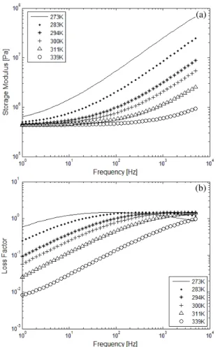
(1.b) From the reduced temperature nomogram generated by the
computation of expressions (1), the designer can obtain the complex modulus and the loss factor at any given temperature into a frequency band of interest, as illustrated in Fig. 1 for the particular material considered above.
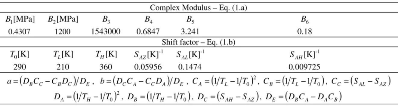
Table 1. Parameters of the 3M™ ISD112 provided by Drake and Soovere (1984). Complex Modulus – Eq. (1.a)
[MPa] 1
B B2[MPa] B3 B4 B5 B6
0.4307 1200 1543000 0.6847 3.241 0.18
Shift factor – Eq. (1.b)
[K] 0
T TL[K] TH[K]
-1 [K]
AZ
S SAL[K]-1
-1 [K]
AH
S
290 210 360 0.05956 0.1474 0.009725
(
DBCC CBDC)
DEa= − , b=
(
DCCA−CCDA)
DE,(
)
2 0 1
1T T
CA= L− , CB=
(
1TL−1T0)
, CC =(
SAL−SAZ)
(
)
20 1
1T T
Figure 1. (a) Storage modulus; (b) loss factor for different temperatures for the 3M™ ISD112.
According to the EVCP the derivation of the FE model accounting for the viscoelastic behavior can be carried-out in two distinct phases: first, the element and global stiffness matrices are obtained by considering pure elastic behavior (i.e., frequency- and temperature-independent material moduli), accounting for the strain state assumed by the underlying theory; then, the material moduli
are modified to account for the viscoelastic behavior according to the complex modulus approach. Clearly, this approach leads to frequency- and temperature-dependent FE stiffness matrices. Assuming isotropic behavior and frequency- and temperature-independent Poisson ratio, the global equations of motion in the frequency domain of a viscoelastic damped system containing DOFs, for which one of the moduli appears factored-out of the viscoelastic stiffness matrix, can be expressed as follows (de Lima et al., 2009):
N
( )
[
Ke+Gω,T Kv−ω M]
Q( )
ω,T =F( )
ω2
(2)
where M∈RN×N is the mass matrix, is the stiffness matrix corresponding to the purely elastic parts, and
N N e R
×
∈
K
N N v R
×
∈
K is
the frequency- and temperature-independent part of the viscoelastic stiffness matrix. and are, respectively, the vectors of the amplitudes of the harmonic generalized displacements and external loads. The receptance or frequency response function matrix is expressed as:
( )
NR T
, ∈
ω
Q F
( )
ω
∈RN( )
[
( )
2]
−1− +
= K K M
Hω,T e Gω,T v ω (3)
(a)
The computation of the FRF by direct inversion of the dynamic stiffness matrix, as indicated in Eq. (3), is unfeasible in practical situations in which FE models with large numbers of DOFs are dealt with. Thus, alternative procedures based on model reduction are proposed in the paper to alleviate the computational cost.
FE Formulation of a Three-layer Sandwich Plate
In this section, the model of a thin or moderately thin three-layer sandwich plate FE, which can be frequently found, for example, in aerospace systems, is summarized, based on the original developments made by Khatua and Cheung (1973). Figure 2 depicts a rectangular element formed by an elastic base-plate (1), a viscoelastic core (2) and an elastic constraining layer (3). This element contains four nodes and seven DOFs per node, representing the in-plane displacements in the middle plane of the base-plate in directions x and y (denoted by u1and v1,respectively), the in-plane displacements of the middle in-plane of the constraining layer in directionsx and y(denoted by u3 and v3, respectively), the transverse displacements,w, and the cross-section rotations aboutx
and y, denoted by
θ
xandθ
y, respectively. (b)(3) constraining layer
(1) base plate (2) viscoelastic core
1 2
3 4
x
y z
a b
w
u1
v1
v3
u3 θ
x
θy
h1
h2
h3
(b)
Figure 2. Three-layer sandwich plate finite element.
In the development of the theory, the following assumptions are adopted: (i) all the materials involved are homogeneous and isotropic and present linear mechanical behavior; (ii) normal stresses and strains in direction z are neglected for all the three layers; (iii) the elastic layers (1) and (3) are modeled according to Kirchhoff’s theory; (iv) for the viscoelastic core, Mindlin’s theory is adopted (transverse shear is included); (v) the cross-section rotations and are assumed to be the same for the elastic layers; (vi) the transverse displacement is the same for all the three layers. These assumptions have been considered by many authors as being adequate for the modeling of thin panels, as it is the case of the structures addressed in the present paper, where it is assumed the facesheets to be thin (Austin, 1999). Moreover, previous studies carried-out by the authors have demonstrated good correlation between model predictions and their experimental counterparts (Lima et al., 2003).
x
θ
θ
yw
( ) ⎪ ⎪ ⎪ ⎭ ⎪ ⎪ ⎪ ⎬ ⎫ ⎪ ⎪ ⎪ ⎩ ⎪ ⎪ ⎪ ⎨ ⎧ ∂ ∂ ∂ ∂ ∂∂ ∂ + ⎪ ⎪ ⎪ ⎭ ⎪ ⎪ ⎪ ⎬ ⎫ ⎪ ⎪ ⎪ ⎩ ⎪ ⎪ ⎪ ⎨ ⎧ ∂ ∂ + ∂ ∂ ∂ ∂∂ ∂ = y x w y w x w z x v y u y vx u k k k k k k 2 2 2 2 2 2
ε
,
(
k=1,3)
(4.a)( ) + ⎪ ⎪ ⎪ ⎪ ⎪ ⎭ ⎪⎪ ⎪ ⎪ ⎪ ⎬ ⎫ ⎪ ⎪ ⎪ ⎪ ⎪ ⎩ ⎪⎪ ⎪ ⎪ ⎪ ⎨ ⎧ ∂ ∂ ∂ + ∂ ∂ − ∂ ∂ + ∂ ∂ − ∂ ∂ ∂ ∂ + ∂ ∂ − ∂ ∂ ∂ ∂ + ∂ ∂ − ∂ ∂ + ⎪ ⎪ ⎪ ⎪ ⎭ ⎪ ⎪ ⎪ ⎪ ⎬ ⎫ ⎪ ⎪ ⎪ ⎪ ⎩ ⎪ ⎪ ⎪ ⎪ ⎨ ⎧ ∂ ∂ + ∂ ∂ ∂ ∂∂ ∂ = 0 0 2 2 0 0 2 1 1 3 1 3 2 2 1 1 3 2 2 1 1 3 2 2 2 2 2 2 2 y x w d x v x v y u y u y w d y v y v x w d x u x u h z x v y u y vx u ε ⎪ ⎪ ⎪ ⎪ ⎭ ⎪⎪ ⎪ ⎪ ⎬ ⎫ ⎪ ⎪ ⎪ ⎪ ⎩ ⎪⎪ ⎪ ⎪ ⎨ ⎧ ∂ ∂ + − ∂ ∂ + − + y w d v v x w d u u h 2 2 0 0 0 1 1 1 3 1 1 3 2 (4.b)
whereε( )k =
[
εx( ) ( ) ( )k εyk γxyk]
T, ε( )2 =[
εx( ) ( ) ( ) ( ) ( )2 εy2 γxy2 γxz2 γyz2]
T,⎟ ⎠ ⎞ ⎜ ⎝ ⎛ ∂ ∂ + + = x w d u u u 2 2 1 2 3 1
2 , ⎟⎟
⎠ ⎞ ⎜⎜ ⎝ ⎛ ∂ ∂ + + = y w d v v v 2 2 1 2 3 1 2 ,
and . In equations (4), designate the transverse coordinates measured from the lower surface of each layer, and subscripts m, b and s designate membrane, bending and shear effects, respectively. The discretization of the displacement fields within the element is made by using the following linear and cubic interpolation functions:
3 1
1 h h
d = +
3 1
2 h h
d = − zk
(
k=1,3)
3 12 3 11 3 10 2 9 2 8 3 7 2 6 5 2 4 3 2 1 16 15 14 13 3 8 7 6 5 1 12 11 10 9 3 4 3 2 1 1 xy b y x b y b xy b y x b x b y b xy b x b y b x b b w xy a y a x a a v xy a y a x a a v xy a y a x a a u xy a y a x a a u + + + + + + + + + + + + = + + + = + + + = + + + = + + + = (5)
where the coefficients and are to be expressed in terms of the nodal displacements and rotations by enforcing the boundary conditions at elementary level.
i
a bi
Based on the kinematic hypotheses and stress-states assumed for each layer, the stress-strain relations are applied, and the strain and kinetic energies of the plate are formulated as:
( )e δ
( )
tT[
( ) ( )e]
δ( )
t v ee K
K
U = +
2 1
, T( )e δ&
( )
tTM( )eδ&( )
t2 1
= (6)
where: ( )
∑
∫ ∫
( ) ( )
= = = = = = 31 0 0
k a x x b y y T k k e dydx y , x y , x
h N N
ρ
Μ (7.a)
is the elementary mass matrix. As for the stiffness matrix,
( )e ( )e ( )e e
Κ
1Κ
3Κ
= + andΚ
v( )e =Κ
2( )e(
ω
,T)
)
are, respectively, the contributions of the purely elastic and viscoelastic parts of the structure, defined, respectively, as:
( )
(
x,y,z)
(
x,y,z)
dydxdz, k h z z a x x b y y k k T k e e k
∑ ∫ ∫ ∫
= = = = = = = = 31 0 0 0
D C D
Κ (7.b)
( )
( )
=∫ ∫ ∫
(
) ( ) (
)
= = = = = = 20 0 0
2 2 2 2 h z z a x x b y y T
e ω,T D x,y,zC ω,T D x,y,z dydxdz
Κ (7.c)
where and are the thickness and the mass density of the k -th layer, respectively. Matrices are formed by differential operators appearing in the strain-displacement relations, and
k
h
ρ
k(
x,y,z)
k
D
(
k=1,2,3( )
x,yN is the matrix containing the shape functions. k
C
(
k=1,3)
and C2( )
ω
,T are, respectively, the matrices ofisotropic elastic and viscoelastic material properties.
Κ
2( )e( )
ω
,T isthe frequency- and temperature-dependent stiffness matrix of the viscoelastic layer. From the elementary matrices computed for each element of the FE mesh, the global equations of motion are constructed, accounting for node connectivity, using standard finite element assembling procedure.
Parameterization of the FE Model
At this point, it is important to consider that, in the context of the present study, the FE model generated according to the formulation above is to be used in combination with optimization procedures, in which objective functions computed from the dynamic responses must be minimized with respect to a set of physical and/or geometrical design parameters which intervene in a rather complicated nonlinear fashion in those responses. In an attempt to reduce the computation cost involved in the optimization, it becomes interesting to perform a parameterization of the finite element model, which is understood as a means of making those parameters to appear explicitly in the mass and stiffness matrices. This procedure enables to account for modifications and/or uncertainties in the values of the design variables in a straightforward way during iterative optimization and/or model updating. Also, it facilitates the evaluation of the sensitivities of the responses with respect to the design parameters (de Lima et al., 2010a).
According to the theory of the sandwich plate finite element summarized in Section 3, the design parameters of mass and stiffness of each layer can be factored-out of the elementary matrices by uncoupling membrane, bending and shear effects, respectively, as follows:
( ) ( ) ( )
( ) ( ) ( ) ( ) ( )
( ) ( ) ( )e
( ) ( ) ( )
( )
(
( ) ( ) ( ))
(
( ) ( ) ( ))
( ) ( ) ( )
(
)
( ) ( ) ( )e
, b e , m e e , s e , s e , s e , b e , b e , b e , m e , m e , m e e , b e , m e h E h E d d d h d d h d d h h E h E 2 3 3 3 3 1 3 3 3 3 2 2 2 3 2 2 1 2 3 0 2 2 2 2 2 2 1 2 2 0 2 2 2 2 2 1 1 2 1 0 2 2 2 2 1 3 1 1 1 1 1 1 1 1 K K K K K K K K K K K K K K K K + = + + + + + + + + + = + = (8.b)
where and ( ) designate the
longitudinal moduli of the elastic layer. Using the notation previously defined, subscripts m, b and s, respectively, indicate the membrane, bending and shear effects in the structural matrices. It should be noted that, in Eqs. (8), the matrices appearing in the right-hand side are constant sparse matrices which are independent from the design parameters. It is clearly perceived how the use of such expressions facilitates the computations related to reanalysis and sensitivity of the response with respect to those parameters.
3 2 1
3 h 2h h
d = + + Ek k=1,3
Robust Condensation of Viscoelastic Systems
In the case of complex structures of industrial interest, FE models are usually constituted by a large number of DOFs (hundreds of thousand or even millions). In such cases, it becomes practically impossible to compute the FRFs directly from Eq. (3), owing to the prohibitive computation times and storage memory required. This fact motivates the use of model reduction techniques, which aims at reducing the model dimensions and the associated computational burden, while keeping a reasonable predictive capacity of the numerical model. This can be done based on the assumption that the exact responses, given by the resolution of Eq. (2) can be approached by projections on a reduced vector basis of the following form (de Lima et al., 2010b):
( )
ω
,T TQˆ(
ω
,TQ =
)
(9)where is the transformation matrix formed by column-wise by base vectors, are generalized coordinates, and is the number of vectors in the basis. By considering Eqs. (2) and (9), the receptance matrix (3) can be rewritten as follows: NR N C × ∈ T
( )
NRC T ,
ˆ
ω
∈Q N
NR<<
( )
[
( )
2 −1− +
= T K T T K T T MT
H v T
T e T T , G T ,
ˆ ω ω ω
]
(10)The reduced dynamic stiffness matrix can be computed frequency by frequency and inverted in a direct way using efficient numerical algorithms. However, for viscoelastic systems, the selection of the basis of reduction is an important aspect. Owing to the dependence of the stiffness matrix with respect to frequency and temperature, the reduction basis should be able to represent the changes of the dynamic behavior as frequency and temperature vary. To comply with this need, various procedures can be adopted regarding the computation of the reduction basis: (i) one can simply neglect this dependence by considering the stiffness matrix as being constant (Balmès and Germès, 2002). In this case, the reduction basis is also constant; (ii) one can use a constant reduction basis obtained by the resolution of the nonlinear eigenvalue problem associated to a frequency- and temperature-dependent stiffness matrix (Palmeri and Ricciardelli, 2006; Daya and Potier-Ferry, 2001; Plouin and Balmès, 1998); (iii) one can use an iterative method for the re-actualization of the basis according to frequency and temperature (Balmès and Germès, 2002). In this work, the strategy proposed consists in using a reduction basis formed by a
constant modal basis of the associate conservative system. However, this basis is enriched by static residual vectors to account for the effects of the external loads and viscoelastic damping forces. These static responses are computed from the low-frequency asymptotic stiffness matrix, representing the static behavior of the viscoelastic materials, according to:
v e
0 K G K
K = + 0 (11)
where is the real part of the modulus function represented by Eq. (1.a). Then, the nominal basis can be obtained by the resolution of the following eigenvalue problem:
0 G
[
]
[
NR]
(
NR)
i i , , diag , N , , i
λ
λ
λ
K K K 1 0 2 1 00 0 1
= = = = −
Λ
ϕ
ϕ
ϕ
ϕ
ϕ
M K (12)In general, a relatively large number of eigenvectors must be kept in the projection basis to guarantee the accuracy of the reduced model. It has been shown in previous studies (Balmès and Germès, 2002; de Lima et al., 2010b) that the number of necessary projection vectors can be reduced by introducing the residues formed by the static displacements associated to external forces, , where is a Boolean matrix which enables to select, among the DOFs, those in which the excitation forces are applied, and the residues associated to the viscoelastic damping forces,
b K R= 0−1
f N R × ∈ b 0 1 0 0
ϕ
v v K KR = − . These residuals are interpreted as the columns of the flexibility matrix of the associated undamped system, associated to the coordinates of application of two types of forces: the external excitation forces and the damping forces. The latter can be better understood by examining Eq. (2), noting that the term involving the viscoelastic behavior can be moved to the right-hand side, where it plays the role of additional forces impressed to the associated conservative structure. Thus, the enriched basis of reduction for the viscoelastic system is given as:
[
0]
0
0 R Rv
T =ϕ (13)
Experience has demonstrated that the nominal reduction basis (13) can be used to reduce the viscoelastic damped systems with reasonable accuracy. Nevertheless, this reduction basis does not represent the modifications of the dynamic behavior provoked by the parametric modifications which must be introduced into the model during iterative processes of optimization and/or model updating. This means that this basis should in principle be updated successively to guarantee a satisfactory accuracy of the reduced model during the iterative processes, which would require costly computations. In order to cope with this difficulty, the strategy suggested herein consists in performing a further enrichment of the reduction basis (13) by a set of residual vectors associated to the modifications of the design parameters, following the procedure proposed by Masson et al. (2003) for undamped systems.
For the modified structural configuration, the dynamic equilibrium equation in the frequency domain can be written as follows:
( ) ( )
ω
,T Qω
,T F( )
ω
FΔ(
ω
,TEquation (14.a) can be interpreted as the dynamic equilibrium equation of the nominal model, subjected to the forces associated to the structural modifications, defined as follows:
( )
ω
,TΔ
( ) (
ω
,Tω
,TΔ Z Q
F =−
)
(14.b)where is the variation of the
dynamic stiffness matrix associated to the parametric modifications.
( )
,TΔΚ
v( )
,TΔΜ
vΔ
Zω
=ω
−ω
2In general, the perturbed matrices associated with the viscoelastic zones are nonlinear functions of the design parameters
. The viscoelastic stiffness and mass matrices, considering modifiable zones of the model can be expressed as follows:
i
p
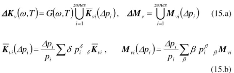
( ) ( )
zonesU
( )
i
i vi
v ,T G ,T p
1 =
=
ω
Δ
ω
KK
Δ
,U
(
(15.a)zones
i
i vi
v p
1 =
= M
Δ
M
Δ
)
( )
=∑
i vi ii i
vi p
p p
p K
K
Δ
Δ
δ
δ δ ,( )
i vii i i
vi p
p p
p M
M β
β β
β
Δ
Δ
=∑
(15.b) In the equations above, the symbol indicates matrix
assembling; subscript indicates the modified viscoelastic zones in which the parameter intervenes;
U
i
i
p Kvi and designate the stiffness and mass matrices corresponding to those viscoelastic zones, respectively. These later are decomposed according to Eq. (15.b) by identifying the matrices
vi
M
vi K
δ and βMvi from which the
δ
- andβ-order exponentials in the parameter can be factored-out. As can be seen in Eq. (14.b), the vector of forces associated to the structural modifications depends on the response of the modified system, . Since this response is unknown apriori, those forces cannot be computed exactly. The essential concept of the robust condensation is expressed in the following steps: first, one uses Eq. (14.b) to generate a vector of forces which, even though it does not contain the exact forces associated to the modifications, will at least represent a subspace containing these vectors. This is accomplished by introducing the response of the nominal system into expression (14.b); next, the resulting vector of forces is used to generate static responses, once again on the basis of the nominal model. These two steps are repeated for each design parameter subjected to modifications. In practice, many types of responses can be introduced into expression (14.b), including the normal modes of the structure and the sensitivity vectors. If the vector introduced is composed of a truncated basis of normal modes, one can rewrite Eq. (14.b) as follows:i
p
(
ω
,TQ
)
)
( )
ω
,T( ) (
ω
,T ˆω
,TΔ Z Q
F ≈−
Δ
ϕ
0 (16)For example, for a parameter intervening in the viscoelastic mass and stiffness matrices, the bases of forces can be expressed under the form
i
p
[
vi]
i i p p
K M
F F
FΔ= Δ Δ , where p vi
ϕ
0Λ
0 andi M
FΔM =
0 0 vi
ϕ
pi G KFKvi =
Δ are the bases of forces associated to the viscoelastic mass and stiffness modifications. After obtaining the bases of forces, one can calculate a series of static responses of the nominal viscoelastic system based on the tangent stiffness matrix as follows , and the final robust condensation basis taking
into account a priori knowledge of the viscoelastic modifications can be expressed as follows:
Δ Δ K F
R 01
−
=
[
T RΔ]
T= 0 (17)
where
[
]
np
p p
p Δ Δ
Δ
Δ R R R
R K
2 1
= and indicates the number
of design parameters to be modified.
np
The residue matrix is not necessarily of maximum rank. Thus, with the aim of obtaining a limited number of independent residue vectors, it is appropriate to select the dominating directions of this basis, which can be done by performing the Singular Value Decomposition (SVD) of to identify its dominant singular values.
Δ R
Δ R
Figure 3 illustrates a comparison between a cycle of optimization or model updating processes by using a standard reduction and the proposed robust condensation strategy. The robust strategy is used to approximate the behavior of the modified viscoelastic structure without the re-actualization of the nominal basis of reduction, leading to a drastic reduction of the time required for computing the responses. Moreover, this approach can be advantageously adapted to several other structural domains based on iterative processes: stochastic structural dynamics, nonlinear mechanics, and reliability-based optimization.
Nominal Model
0
Structural Modification Standard Basis [ T ]
S
T
A
N
D
A
R
D
R
O
B
U
S
T
Standard Basis[ T0 ]
Condensation
Robust basis [ T0 R Δ]
Condensation Resolution
Optimization and/or Model updating
Figure 3. Block-diagram of reanalysis processes associated to robust condensation.
In the case of global modifications, for which the whole structure fully treated by viscoelastic materials is modified by using the same level of perturbation, the standard condensation procedure using the reduction basis (13) is robust and do not need to be improved. In this case, there is only a frequency shift between the nominal model and the perturbed model, so that transformation (13) can represent correctly the perturbed viscoelastic model. However, when local modifications are introduced, which is the case of structures partially treated by constrained viscoelastic layers, experience shows that the accuracy of this solution degenerates rapidly with the amplitude of the perturbation, which demonstrates the interest in using the robust basis (17).
Multiobjective Optimization
Pareto solutions (Eschenauer et al., 1990). Since none of the Pareto solutions can be said to be better than the others without any further consideration, the interest becomes to find as many Pareto optimal solutions as possible from which one can choose based on engineering judgment or other particular criterion. A multiobjective problem includes a set of k parameters and a set of n objective functions (n≥2), and can be symbolically stated as
[
]
( )
[
( ) ( )
( )
( )
[
( )
]
( )
j , ,m and Cg satisfying
opt that
such
f , , f , f of
imization min
by
x , , x , x find
U L
j
n n
∈ ≤ ≤ =
≤ =
= =
∗ ∗ ∗ ∗ ∗
x x x x x
x F x
F
x x
x x F x
K
K K
1 0
2 1 2
1
]
]
(18)
where is the vector of design variables; are the cost functions, normally nonlinear, multimodal and not necessarily analytic; is the design space, which is limited by lateral and inequality constraints
[
Tk
x , , x , x1 2K
=
x
( )
, i , , ,n fi x =12Kk R
C⊂
( )
xj
g .
Evolutionary algorithms (EAs) are widely used to deal with engineering optimization problems due to their ease of implementation and robustness (Eschenauer et al., 1990). The algorithm used to solve the optimization problem dealt within this paper is the so-called Non-dominated Sorting Genetic Algorithm (NSGA) originally developed by Srinivas and Deb (1993). The NSGA mainly differs from the classical multiobjective genetic algorithm in the way the selection operator is used. After ranking the whole population, a same dummy fitness value is provisionally assigned to the members of the first front of Pareto. This fitness value provides an equal reproductive pressure for these individuals, and with the aim of maintaining the diversity of the population, a sharing technique is applied and the fitness value is recomputed accordingly. The fitness is shared when an individual has at least one close neighbor, resulting in the multiplication of its fitness index by the factor . The sharing is performed according to Srinivas and Deb (1993):
(
[
∑
== N
j i j
i shd x,x m
1
)
]
( )
[
]
( )
( )
( )
⎩ ⎨ ⎧
≥ < −
=
σ σ σ
j i
j i j
i j
i if d x,x
x , x d if x , x d x
, x d sh
0 1
(19)
where d
( )
xi,xj is the Euclidian distance between the two individuals xi and xj, andσ
is a constant named sharing coefficient, whose value must be chosen by the analyst.For a viscoelastic system, once the frequency band of interest has been selected, the FRFs whose amplitudes are to be attenuated can be used to define performance indexes (Rade and Steffen, 2000) to be optimized for the selection of a set of optimal continuous design variables and a set of optimal positions of the surface viscoelastic treatments. For the problem considered here, where resonance peaks of the FRF are to be minimized within a frequency band , a possible performance index can be defined as follows:
Rp
(
,Tˆ
ω
H
)
U L
ω
ω
ω
≤ ≤(
xv,xp)
min{
abs[
Hˆ(
ω ,T)
]
, ,abs[
Hˆ(
ωRp,T)
]
}
J = 1 K (20)
where indicates the vector containing the design variables, and represents a set of discrete positions of the viscoelastic treatments.
v
x xp
NSGA Coupled with Metamodels
Since NSGA is a stochastic iterative method requiring a large number of evaluations of the problem solutions, the cost of computations frequently becomes a limiting factor. Hence, the authors found convenient to combine NSGA with approximate models in order to reduce the computation burden associated to the optimization process. In the literature one can find several works describing coupling between optimization algorithms and metamodels (Soteris, 2004). The use of ANNs for nonlinear problems containing a large number of continuous and/or discrete variables is found to be more interesting due to the typically smaller computing time, as compared to response surface methodologies. In this work, MLP artificial neural networks are used in combination with NSGA with the aim of approximating the amplitudes of the damped responses in the frequency domain. The mechanism of search for the optimal solutions by this strategy can be briefly described as follows: (i) the MLP is trained and tested with exact evaluations of the robust condensed model; (ii) NSGA is used to explore the good solutions in the design space; (iii) once NSGA produces a new solution, the MLP is used to determine its fitness value so that NSGA continues the search until a stop criterion is satisfied. A re-initialization of the MLP is necessary to reduce the error between the approximate and exact solutions. This procedure is illustrated in Fig. 4.
Generation k
Generation k+1
Selection Initialization with metamodel?
Selection Crossover Mutation
Optimal solutions
Reduced model/Base of training
Re-initialization ANN not
yes
Figure 4. Illustration of a general NSGA-MLP coupling procedure.
Numerical Application
Evaluation of the Robust Reduction Basis
In this section, the interest is to verify the robustness of the reduced viscoelastic model generated by the use of the proposed condensation method described in Section 5. Figure 5 depicts the test structure composed of a freely suspended stiffened panel containing four stringers. The FE model without viscoelastic treatment is composed of 928 elements having a total number of 5940 DOFs. The viscoelastic treatments, also indicated in Fig. 5, is composed of 10 viscoelastic patches, each one comprising 16 three-layer sandwich plate elements, developed according to the theory presented in Section 3. The FE model of the treated panel contains a total number of 6840 DOFs. The geometric dimensions are: internal radius: 938 mm; length: 720 mm; arc length: 680 mm; thicknesses of the panel and the stringers: 1.5 mm and 0.75 mm, respectively; height of the stringers: 30 mm. The material properties for both panel and stringers are: Young modulus E = 2.1 × 10¹¹
N/m2; mass density ρ = 7800 Kg/m3; Poisson ratio υ = 0.3. The material properties
thicknesses of the viscoelastic and constraining layers are h2 =
0.0254 mm and h3 = 0.5 mm, respectively.
To account for the inherent damping of the untreated structure, the hysteretic damping model was used for the metallic components, represented by a complex, frequency-independent moduli of the formEk=Ek
(
1+iη
k)
, withη
k =0.002(k = 1, 3).Figure 5. FE model of a stiffened panel treated with constrained viscoelastic layers.
The first test is intended to evaluate the nominal enriched basis of reduction by using the static residues associated with the external and viscoelastic forces, according to Eq. (13). The computations consisted in obtaining the driving point FRFs associated with point P, indicated on Fig. 5, assuming the temperature of the viscoelastic material of 25ºC, and the frequency band of interest [135-210Hz]. One considers three nominal bases: (60 eigenvectors); (60 eigenvectors, 1 residual vector computed according to );
(60 eigenvectors, 1 residual vector computed according to , 54 residual vectors computed by
[ ]
0 01=ϕ
T T02 =
[
ϕ
0 R]
]
R K b1 0
−
=
[
00
03 R Rv
T =
ϕ
b K
R 01
−
=
0 1 0
0
ϕ
v v K K
R = − after SVD filtering). It is to be noted that the residues were computed based on the largest singular values, for which the relation
0
v
R
5 1
σ
i≤1×10σ
for i=1to60 holds.Figure 6 shows the amplitudes of the FRFs computed by using the three nominal bases, as compared to the amplitudes of the FRF computed by using a reference reduction basis formed by a far larger number of eigenvectors (600) and residual vectors (600). It can be clearly seen that the accuracy is continuously improved upon successive enrichment of the reduction basis by the inclusion of residual vectors accounting for the static residues associated with the external loading and damping forces, to form the nominal basis T02 and T03, respectively.
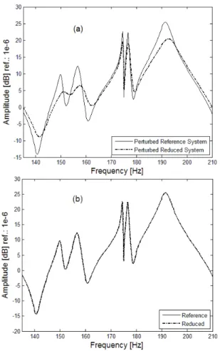
The interest now is to evaluate the robustness of the nominal basis further enriched to account for structural modifications introduced into the nominal model, according to Eq. (17). The modification considered consists in increasing the thickness of the constraining layer of the nominal system in 90%. Figure 7 enables to compare the amplitudes of the FRFs for the nominal and perturbed damped systems; both computed using the same reference reduction basis, without further enrichment for structural modifications. It can be seen that the dynamic behavior of the perturbed damped system does not differ appreciably from that of the nominal system, although damping levels are strongly influenced. In Fig. 8(a), the FRF of the perturbed reference system
is compared to the counterpart computed by using the nominal basisT03=
[
ϕ
0 R Rv0]
containing 115 vectors. The observed differences lead to conclude that this basis is not capable of representing accurately enough the changes of the dynamic behavior induced by the structural modifications introduced. Figure 8(b) enables to compare the FRF of the perturbed reference system to the counterpart computed by using the basis containing 146 vectors (including 31 SVD-filtered residual vectors associated to the structural modifications).[
RΔT4=
Τ
03]
This time, one can observe a very satisfactory agreement between the amplitudes of the FRFs of both models. This leads to conclude that the reduction basis is robust enough to represent the response of the perturbed system in the frequency band of interest.
4
T
Figure 7. FRFs computed for the nominal and perturbed systems for the reference reduction basis.
Figure 8. FRFs computed for the nominal and perturbed systems using the basis: (a) T03; (b) T4.
Optimization combining NSGA, robust condensation
and ANNs
After having verified the robustness of the model reduction technique applied to viscoelastic systems, the interest now is to evaluate the proposed multicriteria optimization strategy coupling NSGA, robust condensation and ANNs, as described in Section 6.1, for the optimization of the stiffened panel treated with viscoelastic constrained layers. In this application, the viscoelastic treatment is composed of 15 viscoelastic patches, each one composed of 16
three-layer sandwich plate FEs. The objective functions are the peak amplitudes of FRFs for modes 10, 11 and 14, with the aim of increasing the damping performance for these modes by minimizing the amplitudes of the FRFs in the vicinity of the corresponding resonance peaks. The choice of these modes is justified by the amount of modal strain energy observed for them (Johnson and Kienholz, 1982). The optimization problem is formulated as a mixed discrete-continuous one according to Eq. (20). The continuous design variables considered, expressed in terms of their nominal values and admissible variations are: thicknesses of the viscoelastic layer, (h2 = 0.0254 mm, ±70%), and constraining layer (h3 = 0.5 mm,
±50%), and the temperature of the viscoelastic material (T = 25ºC, ±15%). As discrete variables to be optimized one considers the positions of each viscoelastic patch. Only the admissible ranges of the continuous variables defined previously are taken as lateral constraints in the optimization problem. The optimal positioning of the patches is chosen among a previously selected set of candidate positions, accounting for the FE mesh. Both types of variables are dealt with in an integrated fashion within NSGA. It should be noted that, although the temperature is a parameter upon which one has little control in practical applications, it is considered as a design variable, since, as temperature has a strong influence on the viscoelastic behavior, it becomes important to evaluate the robustness of the optimal solutions with respect to its variations.
The parameters of the NSGA are defined as follows: population size: 30; selection probability: 0.25; crossover probability 0.25; mutation probability: 0.25; sharing coefficient: σ = 0.2. For the MLP-ANN, it was chosen to use two hidden layers and twenty neurons per layer. The objective functions are calculated based on the robust reduced viscoelastic damped model for which the nominal basis of reduction, constructed according to Eq. (13), is composed of 121 vectors (60 eigenvectors, 1 vector related to the static residue, and 60 residual vectors related to the viscoelastic forces). The robust basis of reduction is enriched during the optimization process accounting for structural modifications of the continuous design variables, according to Eq. (17). The total number of generations of the NSGA was limited to 100, which means that the maximum number of evaluations of cost functions was 3000. For that, the neural network is updated at each 20 generations after generation 5, enabling to reduce the number of exact evaluations from 3000 to 170. The CPU time required for the two optimization runs were found to be: for NSGA only: 1634.4 min; for the combination NSGA-MLP: 146 min. This leads to conclude that the NSGA-MLP procedure allows a significant reduction of the computation time during the optimization process, with a reduction ratio of approximately 89%.
Figures 9(a) and 9(b) show the solutions obtained by using only NSGA (thus without any metamodeling approximation) and those obtained by using the coupling procedure NSGA-MLP. For both groups, one uses the robust reduced model. By comparing the first front of Pareto for the amplitudes of modes 10 and 11, one can conclude that the NSGA-MLP approach represents quite well the response of the viscoelastic system, as demonstrated by the similarity of the two clouds of solutions.
Figure 10. FRFs for the optimal design solutions: (a) A, (b) B, (c) C. Figure 11 illustrates the optimal positions of the viscoelastic patches for the solution B and the optimal values of the thicknesses of the viscoelastic and constraining layers for each patch are given in Table 2. For this optimal solution, the optimal value of temperature of the viscoelastic material was found to be 21.25ºC.
Figure 9. Solutions obtained by using NSGA and NSGA-MLP: (a) three objective functions; (b) front of Pareto for the cost functions M10 and M11.
Figure 11. Optimal positions of the viscoelastic treatments corresponding to solution B.
Table 2. Optimal values of the design parameters for solution B. Patches
1,2,3,5 4,6,7,10,12,13,15 8,9,11,14 h2 [m]
×10-5
h3 [m]
×10-3
h2 [m]
×10-5
h3 [m]
×10-3
h2 [m]
×10-5
h3 [m]
×10-3
1.02 0.55 1.02 0.65 1.19 0.65 1.49 0.65 1.02 0.65 1.21 0.65 1.02 0.61 1.02 0.65 1.02 0.65 1.02 0.65 1.02 0.65 1.87 0.65
Concluding remarks
A multiobjective optimization procedure combining evolutionary algorithms, robust condensation and metamodeling, intended to be adapted for dealing with large systems containing viscoelastic damping was suggested and evaluated. The original aspects of the procedure reside in the adaptation of the concept of robust condensation, initially developed for undamped structures, for systems containing viscoelastic damping and the use multilayer perceptron Artificial Neural Networks to approximate the responses of the system within the optimization procedure, aiming at reducing the computational cost.
positioning and dimensioning of viscoelastic patches. The obtained results demonstrated the effectiveness of the optimization strategy mainly in terms of the drastic reduction of computation time required to obtain the optimal Pareto solutions, which demonstrates that the suggested technique is well adapted to be applied to complex industrial structures.
As current developments, it is being considered the integration of other metamodeling strategies to approximate the response of large viscoelastic damped systems based on the use of classically and adaptive response surface methodologies, and the use of radial basis functions. Also, techniques intended for the evaluation of the robustness of the optimal solutions with respect to uncertainties in the viscoelastic parameters and stochastic analysis of viscoelastic structures are being addressed by the authors.
Acknowledgements
The authors wish to thank the following organizations: Brazilian Research Council – CNPq for the continued support to their research work, especially through research projects 480785/2008-2 (A.M.G. de Lima) and 310524/2006-7 (D.A. Rade), Minas Gerais State Agency FAPEMIG and CAPES Foundation.
References
Austin, E.M., 1999, “Variations on Modeling of Constrained-Layer Damping Treatments”, Shock and Vibration Digest, Vol. 31, No. 4, pp. 275-280.
Bagley, R.L. and Torvik, P.J., 1983, “Fractional Calculus – A Different Approach to the Analysis of Viscoelastic Damped Structures”, AIAA Journal, Vol. 21, No. 5, pp. 741-748.
Balmès, E. and Germès, S., 2002, “Tools for Viscoelastic Damping Treatment Design: Application to an Automotive Floor Panel”, Proceedings of the 28th International Seminar on Modal Analysis (ISMA), Leuven, Belgium.
Daya, E.M. and Potier-Ferry, M., 2001, “A Numerical Method for Nonlinear Eigenvalue Problems: Application to Vibrations of Viscoelastic Structures”, Journal of Computers and Structures, Vol. 79, pp. 533-541.
de Lima, A.M.G., Stoppa, M.H. and Rade, D.A., 2003, “Finite Element Modelling and Experimental Characterization of Beams and Plates Treated with Constraining Damping Layers”, Proceedings of the 17th International Conference of Mechanical Engineering, São
Paulo, Brazil.
de Lima, A.M.G., Rade, D.A. and Lépore-Neto, F.P., 2009, “An Efficient Modeling Methodology of Structural Systems Containing Viscoelastic Dampers Based on Frequency Response Function Substructuring”, Mechanical System and Signal Processing, Vol. 23, No. 4, pp. 1272-1281.
de Lima, A.M.G., Faria, A.W. and Rade, D.A., 2010a, “Sensitivity Analysis of Frequency Response Functions of Composite Sandwich Plates Containing Viscoelastic Layers”, Composite Structures, Vol. 92, No. 2, pp. 364-376.
de Lima, A.M.G., da Silva, A.R., Rade, D.A. and Bouhaddi, N., 2010b, “Component Mode Synthesis Combining Robust Enriched Ritz Approach for Viscoelastically Damped Structures”, Engineering Structures, Vol. 32, No. 5, pp. 1479-1488.
Drake, M.L. and Soovere, J., 1984, “A Design Guide for Damping of Aerospace Structures”, Proceedings of the AFWAL Vibration Damping Workshop, No. 3, Atlantic City, USA.
Eschenauer, J., Koski, J. and Osyczka, A., 1990, “Multicriteria Design Optimization”, Springer-Verlag.
Espindola, J.J., Bavastri, C.A. and Lopes, E.M., 2008, “Design of Optimum Systems of Viscoelastic Vibration Absorbers for a given Material Based on the Fractional Calculus Model”, Journal of Vibration and Control, Vol. 14, No. 9, pp. 1607-1630.
Espindola, J.J., Lopes, E.M. and Bavastri, C.A., 2005, “A Generalized Fractional Derivative Approach to Viscoelastic Materials Properties Measurements”, Applied Mathematics and Computation, Vol. 164, No. 2, pp. 473-506.
Galucio, A.C., Deü J.-F., Ohayon, R., 2004, “Finite Element Formulation of Viscoelastic Sandwich Beams Using Fractional Derivative Operators”, Computational Mechanics, Vol. 33, p. 282-291.
Hao, M., Rao, M.D. and Schabus, M.H., 2004, “Optimum Design of Multiple-Constraint-Layered Systems for Vibration Control”, AIAA Journal, Vol. 42, No. 12, pp. 2448-2461.
Johnson, C.D. and Kienholz, D.A., 1982, “Finite Element Prediction of Damping in Structures with Constrained Viscoelastic Layers”, AIAA Journal, Vol. 20, no. 9, pp. 1284-1290.
Khatua, T.P. and Cheung, Y.K., 1973, “Bending and Vibration of Multilayer Sandwich Beams and Plates”, International Journal for Numerical Methods in Engineering, Vol. 6, pp. 11-24.
Lee, S.H., Son, D.I., Kim, J. and Min, K.W., 2004, “Optimal Design of Viscoelastic Dampers using Eigenvalue Assignment”, Earthquake Engineering and Structural Dynamics, Vol. 33, No. 4, pp. 521-542.
Lesieutre, G.A. and Lee, U., 1996, “A Finite Element for Beams Having Segmented Active Constrained Layers with Frequency-Dependent Viscoelastics”, Smart Materials & Structures, Vol. 5, No. 5, pp. 615-627.
MacTavish, D. and Hughes, P.C., 1993, “Modeling of Linear Viscoelastic Space Structures”, Journal of Vibration and Acoustics, Vol. 115, No. 2, pp. 103-115.
Masson, G., Bouhaddi, N., Cogan, S. and Laurant, S., 2003, “Component Mode Synthesis Method Adapted to Optimization of Structural Dynamics Behavior”, Proceedings of the XXІ International Modal Analysis (IMAC), Hyatt Orlando, USA.
Nashif, A.D., Jones, D.I.G. and Henderson, J.P., 1985, “Vibration Damping”, John Wiley & Sons, New York.
Palmeri, A. and Ricciardelli, F., 2006, “Fatigue Analyses of Buildings with Viscoelastic Dampers”, Journal of Wind Engineering and Industrial Aerodynamics, Vol. 94, No. 5, pp. 377-395.
Plouin, A.S. and Balmès, E., 1998, “Pseudo-Modal Representation of Large Models with Viscoelastic Behavior”, Proceedings of the XVІ International Modal Analysis, Santa Barbara, USA.
Rade, D.A. and Steffen Jr., V., 2000, “Optimization of dynamic vibration absorbers over a frequency band”, Mechanical Systems and Signal Processing, Vol. 14, pp. 679-690.
Rao, M.D., 2001, “Recent Applications of Viscoelastic Damping for Noise Control in Automobiles and Commercial Airplanes”, Proceedings of the India-USA Symposium on Emerging Trends in Vibration and Noise Engineering, Columbus, USA.
Samali, B. and Kwok, K.C.S., 1995, “Use of Viscoelastic Dampers in Reducing Wind and Earthquake Induced Motion of Building Structures”, Engineering Structures, Vol. 17, No. 9, pp. 639-654.
Soteris, K.A., 2004, “Optimization of Solar Systems using Artificial Neural Networks and Genetic Algorithms”, Journal of Applied Energy, Vol. 11, No. 2, pp. 383-405.
Srinivas, N. and Deb, K., 1993, “Multiobjective using Nondominated Sorting in Genetic Algorithms”, Technical Report, Depart. of Mech. Eng., Institute of Technology, India.