TCD
8, 845–885, 2014Sea ice melt pond fraction estimation –
Part 2
R. K. Scharien
Title Page
Abstract Introduction
Conclusions References
Tables Figures
◭ ◮
◭ ◮
Back Close
Full Screen / Esc
Printer-friendly Version Interactive Discussion
Discussion
P
a
per
|
D
iscussion
P
a
per
|
Discussion
P
a
per
|
Discuss
ion
P
a
per
|
The Cryosphere Discuss., 8, 845–885, 2014 www.the-cryosphere-discuss.net/8/845/2014/ doi:10.5194/tcd-8-845-2014
© Author(s) 2014. CC Attribution 3.0 License.
Open Access
The Cryosphere
Discussions
This discussion paper is/has been under review for the journal The Cryosphere (TC). Please refer to the corresponding final paper in TC if available.
Sea ice melt pond fraction estimation
from dual-polarisation C-band SAR –
Part 2: Scaling in situ to Radarsat-2
R. K. Scharien, K. Hochheim, J. Landy, and D. G. Barber
Centre for Earth Observation Science, Faculty of Environment Earth and Resources, University of Manitoba, Winnipeg, Manitoba, USA
Received: 19 December 2013 – Accepted: 6 January 2014 – Published: 27 January 2014
Correspondence to: R. K. Scharien ([email protected])
TCD
8, 845–885, 2014Sea ice melt pond fraction estimation –
Part 2
R. K. Scharien
Title Page
Abstract Introduction
Conclusions References
Tables Figures
◭ ◮
◭ ◮
Back Close
Full Screen / Esc
Printer-friendly Version Interactive Discussion
Discussion
P
a
per
|
D
iscussion
P
a
per
|
Discussion
P
a
per
|
Discuss
ion
P
a
per
|
Abstract
Observed changes in the Arctic have motivated efforts to understand and model its components as an integrated and adaptive system at increasingly finer scales. Sea ice melt pond fraction, an important summer sea ice component affecting surface albedo and light transmittance across the ocean-sea ice–atmosphere interface, is
in-5
adequately parameterized in models due to a lack of large scale observations. In this paper, results from a multi-scale remote sensing program dedicated to the retrieval of pond fraction from satellite C-band synthetic aperture radar (SAR) are detailed. The study was conducted on first-year sea (FY) ice in the Canadian Arctic Archipelago dur-ing the summer melt period in June 2012. Approaches to retrieve the subscale FY ice
10
pond fraction from mixed pixels in RADARSAT-2 imagery, using in situ, surface scatter-ing theory, and image data are assessed. Each algorithm exploits the dominant effect of high dielectric free-water ponds on the VV/HH polarisation ratio (PR) at moderate to high incidence angles (about 40◦ and above). Algorithms are applied to four im-ages corresponding to discrete stim-ages of the seasonal pond evolutionary cycle, and
15
model performance is assessed using coincident pond fraction measurements from partitioned aerial photos. A RMSE of 0.07, across a pond fraction range of 0.10 to 0.70, is achieved during intermediate and late seasonal stages. Weak model performance is attributed to wet snow (pond formation) and synoptically driven pond freezing events (all stages), though PR has utility for identification of these events when considered in
20
time series context. Results demonstrate the potential of wide-swath, dual-polarisation, SAR for large-scale observations of pond fraction with temporal frequency suitable for process-scale studies and improvements to model parameterizations.
1 Introduction
A decline in Arctic sea ice thickness over the past several decades (Kwok and Rothrock,
25
Be-TCD
8, 845–885, 2014Sea ice melt pond fraction estimation –
Part 2
R. K. Scharien
Title Page
Abstract Introduction
Conclusions References
Tables Figures
◭ ◮
◭ ◮
Back Close
Full Screen / Esc
Printer-friendly Version Interactive Discussion
Discussion
P
a
per
|
D
iscussion
P
a
per
|
Discussion
P
a
per
|
Discuss
ion
P
a
per
|
ginning around 2007, the winter volume of sea ice in the Arctic became dominated by thinner first-year (FY) ice, rather than thicker multiyear (MY) ice (Kwok et al., 2009). A FY ice dominant regime has a greater annual areal fraction of melt ponds during summer melt, due to a relative lack of topographical controls on melt water flow com-pared to MY ice (Fetterer and Untersteiner, 1998; Barber and Yackel, 1999; Eicken
5
et al., 2002, 2004; Freitag and Eicken, 2003; Polashenski et al., 2012). Melt ponds have much lower albedo (∼0.2–0.4) than the surrounding ice cover (∼0.6–0.8) (Per-ovich, 1996; Hanesiak et al., 2001b), which promotes shortwave energy absorption into the ice volume and accelerates ice decay (Maykut, 1985; Hanesiak et al., 2001a). Heat uptake by pond covered ice increases the rate at which its temperature related brine
10
volume fraction increases to the∼5 % threshold, the point at which the fluid perme-ability threshold is crossed (Golden et al., 1998) and vertical biogeochemical material exchange of the full ice volume with the underlying ocean becomes possible (see Van-coppenolle et al., 2013, for a review). Melt ponds transmit light to the underlying ocean at an order of magnitude higher rate than bare ice (Inoue et al., 2008; Light et al., 2008;
15
Ehn et al., 2011; Frey et al., 2011), which leads to warming (Perovich et al., 2007) and stimulates under-ice primary production (Mundy et al., 2009; Arrigo et al., 2012) in the upper ocean layer. Increased ocean surface warming has been linked to subsequent reductions in ice volume due to its effect on the timing of seasonal melt onset and fall-freeze up (Laxon et al., 2003; Perovich et al., 2007). The proliferation of melt ponds
20
is also related to the atmospheric deposition, and discharge into the ocean, of con-taminants such as organochlorine pesticides (Pucko et al., 2012) and higher nutrient concentrations (Lee et al., 2012).
Understanding the role of melt ponds in large scale climatological and biogeochemi-cal processes, improving weather forecast models, and conducting climate-cryosphere
25
TCD
8, 845–885, 2014Sea ice melt pond fraction estimation –
Part 2
R. K. Scharien
Title Page
Abstract Introduction
Conclusions References
Tables Figures
◭ ◮
◭ ◮
Back Close
Full Screen / Esc
Printer-friendly Version Interactive Discussion
Discussion
P
a
per
|
D
iscussion
P
a
per
|
Discussion
P
a
per
|
Discuss
ion
P
a
per
|
Skyllingstad et al., 2009; Flocco et al., 2010) and a greater understanding of ice-albedo feedbacks (Holland et al., 2012). However the parameterizations are based on limited field observations that do not account for the horizontal heterogeneity of ice types and pond fractions. The pond fraction on a mixture of FY and MY ice may vary locally from 10–70 % at a snapshot in time (e.g. Derksen et al., 1997; Eicken et al., 2004;
Polashen-5
ski et al., 2012). Over time, variations at one location up to 50 % are typical (Perovich and Polashenski, 2012), with changes greater than 75 % observed on the smoothest FY ice (Scharien and Yackel, 2005; Hanesiak et al., 2001b). Diurnal variations as high as 35 % have been observed on FY ice (Scharien and Yackel, 2005).
Satellite scale observations of melt pond properties require improvements to retrieval
10
methods. Unmixing algorithms have been developed for estimating pond fraction from multispectral optical data (Markus et al., 2003; Tschudi et al., 2008; Rösel et al., 2012) and applied to a basin-scale analysis of pond fraction patterns using MODIS sensor data from 2000–2011 (Rösel and Kalschke, 2012). Optical approaches are limited by assumptions made regarding the predefined spectral behaviour of surface types open
15
water, melt ponds, and snow/ice (Zege et al., 2012). The frequency of optical observa-tions are also limited by persistent stratus cloud cover over the Arctic during summer (Inoue et al., 2005). Passive and active microwave radiometers and scatterometers pro-vide Arctic-wide coverage of summer ice regardless of cloud cover and weather condi-tions. Data from these sensors have been used to identify pond formation (Comiso and
20
Kwok, 1996; Howell et al., 2006), though their low resolution (several kilometres) and vulnerability to signal contamination by land and open water (Heygster et al., 2012) make quantitative melt pond retrievals problematic. Synthetic Aperture Radar (SAR) data has been investigated for its utility in providing synoptic scale melt pond infor-mation. SAR is an all-weather, active microwave, backscatter data source that
pro-25
TCD
8, 845–885, 2014Sea ice melt pond fraction estimation –
Part 2
R. K. Scharien
Title Page
Abstract Introduction
Conclusions References
Tables Figures
◭ ◮
◭ ◮
Back Close
Full Screen / Esc
Printer-friendly Version Interactive Discussion
Discussion
P
a
per
|
D
iscussion
P
a
per
|
Discussion
P
a
per
|
Discuss
ion
P
a
per
|
ponding and for proxy estimates of sea ice albedo and pond fraction (Jeffries et al., 1997; Yackel and Barber, 2000; Hanesiak et al., 2001a). Single polarisation backscat-ter intensity variations caused by variable wind stress on pond surfaces imposes the need for ancillary wind speed measurements to aid retrievals (Comsio and Kwok, 1996; Barber and Yackel, 1999; De Abreu et al., 2001). Using in situ measured C-band
po-5
larimetric backscatter from pond covered Arctic FY ice, Scharien et al. (2012) demon-strated that the polarimetric ratio (PR) behaved independently of surface roughness and that that the PR response of individual pond and bare ice samples was consistent with Bragg behaviour. The PR is a ratio of the linear, co-polarisation, transmit-receive (VV and HH) channels measurable by dual-polarised or polarimetric radars. As outlined
10
in more detail in Sect. 2.2, the PR of a Bragg surface is independent of surface rough-ness and responsive to the dielectric constant (Fung, 1994). Scharien et al. (2012) found the PR of high dielectric free water ponds was much greater than bare ice, and they suggested evaluating a PR-based approach for the retrieval of pond information (e.g. pond formation, pond fraction evolution) from satellite SAR, combined with more
15
rigorous evaluation of the roughness characteristics of the surface in relation to Bragg scattering model theory.
In Part 1 of this study, detailed in situ surface roughness measurements of advanced melt FY ice pond and bare ice features were compared to the rough surface validity limit of the Bragg model at C-band frequency (Scharien et al., 2014; this issue). This
20
was done within the framework of our working hypothesis: as defined by Bragg model theory, FY ice melt pond fraction is retrievable from PR measured at C-band frequency. Part 1 demonstrated that bare ice falls within the Bragg validity limit, while the roughest ponds exceed the limit. Establishing a wind speed threshold for the roughest ponds is unsatisfactory, as morphological factors also contribute to pond roughness. The
dom-25
TCD
8, 845–885, 2014Sea ice melt pond fraction estimation –
Part 2
R. K. Scharien
Title Page
Abstract Introduction
Conclusions References
Tables Figures
◭ ◮
◭ ◮
Back Close
Full Screen / Esc
Printer-friendly Version Interactive Discussion
Discussion
P
a
per
|
D
iscussion
P
a
per
|
Discussion
P
a
per
|
Discuss
ion
P
a
per
|
Though the Bragg limit of FY ice ponds can be exceeded, the scale of analysis in Part 1 represents a significant oversampling in spatial and temporal dimensions, requiring analysis of distributed pond and ice data in satellite SAR.
In this paper, Part 2, a satellite SAR scale evaluation of our working hypothesis is conducted by combining RADARSAT-2 (RS-2) derived backscatter statistics with
coin-5
cident aerial photography (AP). Though emphasis is placed on the PR, linear co- and cross-polarisation (VV, HH, and HV) and cross-polarisation ratio (HV/HH) statistics are included for enhanced interpretation. Within this framework the following objec-tives are addressed: (1) to synthesize calibrated dual-polarisation C-band frequency RADARSAT-2 backscatter statistics over undeformed FY ice during the ponding
sea-10
son, and (2) to evaluate novel approaches for the retrieval of FY melt pond fraction using the PR. The first objective addresses spatial and temporal aspects of RS-2 backscatter and pond fraction. Backscatter statistics and AP derived pond fractions are compared during discrete melt pond evolutionary stages, demarcated by Eicken et al. (2002) and described in Sect. 2.1. This provides the basis for the second
objec-15
tive, which directly addresses the working hypothesis. Section 2.2 describes the Bragg scattering model as it pertains to PR based unmixing of pond fraction. Methods used to acquire and process the experimental dataset, and three experimental methods to re-trieve pond fractions from calibrated RS-2 PR bands are described in Sect. 3. Results in Sect. 4 are ordered as follows: a seasonal description of backscatter statistics and
20
pond fraction evolution (Sect. 4.1); a comparison of spatially distributed polarisation ra-tios and pond fractions along each AP flight lines (Sect. 4.2); and an evaluation of RS-2 retrieved and AP derived pond fractions using statistics RMSE and bias (Sect. 4.3). Pertinent findings and limitations are discussed in Sect. 5, before the main results are recalled and conclusions made in Sect. 6.
TCD
8, 845–885, 2014Sea ice melt pond fraction estimation –
Part 2
R. K. Scharien
Title Page
Abstract Introduction
Conclusions References
Tables Figures
◭ ◮
◭ ◮
Back Close
Full Screen / Esc
Printer-friendly Version Interactive Discussion
Discussion
P
a
per
|
D
iscussion
P
a
per
|
Discussion
P
a
per
|
Discuss
ion
P
a
per
|
2 Background
2.1 Stages of pond evolution
In order to simplify the dynamic nature of ponding, various sub-stages have been iden-tified. These are either based on the thermodynamic (ablation) state of the ice volume (Hanesiak et al., 2001a; Perovich et al., 2007), or the evolution of surface hydrology
5
(Eicken et al., 2002). The stages outlined in Eicken et al. (2002) in an analysis of flow rates and transport pathways on summer FY and MY in the northern Chukchi Sea, are used in this study. These staged, hereafter the “Eicken stages”, provide a logi-cal coupling between evolving surface features and dominant microwave backscatter mechanisms.
10
During the Ponding Stage I, the melting snow cover provides a rapid influx of melt water which laterally spreads over a large area (high pond fraction) on undeformed first-year ice. Past observations have shown that the seasonal peak in pond fraction on FY ice occurs as melt water from the rapidly ablating snow cover is retained by an impermeable ice cover (see summary of published data in Polashenski et al., 2012). As
15
there are almost no topographical controls on melt water flow, ponds spread laterally so that the peak fraction typically reaches>0.5 (Eicken et al., 2004). Ponding Stage II begins when the snow cover has ablated and the pond fraction is driven by the balance between melt rate (rise in pond fraction) and lateral flows through cracks and seal holes (drop in pond fraction). Pond fraction during this stage is driven by a balance between
20
the intensity of melt, which controls meltwater production, and lateral and vertical fluxes of meltwater, which control meltwater drainage (Eicken et al., 2002). Ponding Stage III is demarcated by hydraulic connectivity between the ice and the ocean, and the vertical, in addition to lateral, transport of water through macroscopic holes in the ice. During this stage vertical pathways between the ice cover and ocean form, leading to
25
TCD
8, 845–885, 2014Sea ice melt pond fraction estimation –
Part 2
R. K. Scharien
Title Page
Abstract Introduction
Conclusions References
Tables Figures
◭ ◮
◭ ◮
Back Close
Full Screen / Esc
Printer-friendly Version Interactive Discussion
Discussion
P
a
per
|
D
iscussion
P
a
per
|
Discussion
P
a
per
|
Discuss
ion
P
a
per
|
2.2 Bragg scattering model
For a surface comprising roughness features that are small relative to the incident radar wavelength, its linear polarisation backscatter can be described by the small perturba-tion or Bragg model (Fung, 1994). A Bragg model surface is defined by the smooth surface roughness validity criterionks <0.3, wherek=2π/λandsis the surface
rms-5
height. The scattering mechanism is single (surface) scattering and, as described in Hajnsek et al. (2003), its polarimetric backscatter behaviour is described by a scatter-ing matrix [S]:
[S]=
ShhShv Svh Svv
, (1)
10
where the subscripts refer to the transmit and receive polarizations which are horizontal (h) and vertical (v) for the linear basis. For a Bragg surface, Eq. (1) can be modified as follows:
[S]=ms
Rhh(θ,εr) 0
0 Rvv(θ,εr)
, (2)
15
wherems is the backscatter amplitude andRhh and Rvv are Bragg scattering coeffi
-cients:
Rhh=
cos(θ)− q
εr−sin 2
(θ)
cos(θ)+
q
εr−sin 2
(θ)
, (3)
Rvv=
(εr−1)
n
sin2(θ)−εr[1+sin 2
(θ)]o
εrcos(θ)+
q
εr−sin2(θ)
2 . (4)
TCD
8, 845–885, 2014Sea ice melt pond fraction estimation –
Part 2
R. K. Scharien
Title Page
Abstract Introduction
Conclusions References
Tables Figures
◭ ◮
◭ ◮
Back Close
Full Screen / Esc
Printer-friendly Version Interactive Discussion
Discussion
P
a
per
|
D
iscussion
P
a
per
|
Discussion
P
a
per
|
Discuss
ion
P
a
per
|
From Eqs. (2) and (3), the ratio of Bragg coefficients (Rvv/Rhh) is independent of
sur-face roughness and dependent only on the radar incidence angle θ and the surface complex permittivity or dielectric constant εr. The ratio is equivalent to the PR de-rived from VV and HH transmit-receive radar scattering coefficients (σ◦) recorded by an imaging radar or scatterometer:
5
PR= σ ◦
vv σ◦
hh
. (5)
On the one hand, knowledge of the permittivity of a Bragg surface enables the estima-tion of the PR. Conversely, a PR model may allow the simple retrieval of a geophysical parameter on the basis of changes in its bulk permittivity. Detectable changes in the
10
bulk permittivity are typically dominated by the presence of a high dielectric such as water or brine. Considering a pond covered sea ice surface, a low dielectric sea ice host with εi=3.11+0.208i is covered with varying fractions of high dielectric ponds
withεw=67.03+35.96i. A mixture modelling approach can be used to estimate the
surfaceεr corresponding to a horizontally distributed mixture of ice and ponds (Ulaby
15
et al., 1986):
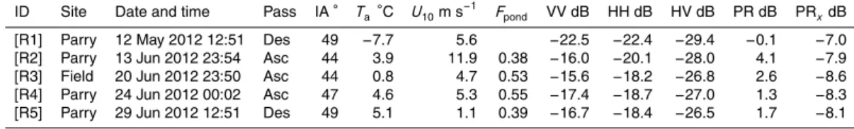
εr=εh+vw(εw−εh). (6)
From this, Eqs. (3) and (4) are then used to create a PR model for pond fraction (Fig. 1). Figure 1 illustrates the use of a PR model for the estimation of parameters related to
20
the formation, pond fraction evolution, and drainage of melt pond from a sea ice surface which conforms to the Bragg surface roughness limit. Ponds are more easily detected at largerθand when the pond fraction is high, as denoted by a relative increase in PR by several deciBels (dB) compared to smallerθand lower pond fractions. It follows that a pond fraction may be retrieved from the PR at a fixedθ, again provided theθis high
25
TCD
8, 845–885, 2014Sea ice melt pond fraction estimation –
Part 2
R. K. Scharien
Title Page
Abstract Introduction
Conclusions References
Tables Figures
◭ ◮
◭ ◮
Back Close
Full Screen / Esc
Printer-friendly Version Interactive Discussion
Discussion
P
a
per
|
D
iscussion
P
a
per
|
Discussion
P
a
per
|
Discuss
ion
P
a
per
|
3 Methods
3.1 Data collection
Data were collected during the Arctic-Ice Covered Ecosystem in a Rapidly Changing Environment (Arctic-ICE) field project from May – June 2012. Arctic-ICE is an interdis-ciplinary project with focus on biogeophysical processes occurring at the ocean-sea
5
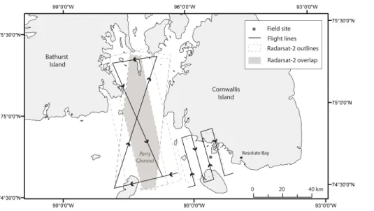
ice-atmosphere (OSA) interface during the spring-summer snow melt and ponding pe-riods. The project was conducted on the relatively undeformed, landfast, FY ice in the central Canadian Arctic Archipelago, adjacent to Resolute Bay, Nunavut. Proximity to Resolute Bay enabled access to the nearby airport and the coupling of in situ data with aerial photography (AP) fights flown over the study site. Figure 2 shows a map of the
10
field study site location, along with the configuration of AP survey lines over the field site (hereafter Field) and Parry Sound (hereafter Parry). Also included in Fig. 2 are the outlines of the RS-2 acquisitions acquired for this study (described in detail below).
AP surveys were conducted to capture digital imagery of the ice surface and quantify relative fractions of pond, ice, and open water. During each survey, a set of lines were
15
flown over Parry at an altitude of 1542 m (∼5000 ft), followed by lines over the study site at 610 m (∼2000 ft). Images were captured using a Canon G10 camera mounted to an open hatch in the rear of a fixed wing DHC-6 Twin Otter aircraft. The camera was operated in time-lapse mode, with camera settings and capture rate controlled using a laptop and proprietary software. At 1542 m flying height, images cover an
es-20
timated 1872 m swath with 0.54 m pixel size; at 610 m flying height the swath is 749 m and pixel size 0.22 m. Adjustments to the time-lapse capture rate were made during flights to ensure a regular 10 % overlap, for example when ground speed or altitude variations occurred. A time-synched GPS on the aircraft was used to logx, y, and z
position data at 1 s resolution, which enabled image registration (geotagging) during
25
TCD
8, 845–885, 2014Sea ice melt pond fraction estimation –
Part 2
R. K. Scharien
Title Page
Abstract Introduction
Conclusions References
Tables Figures
◭ ◮
◭ ◮
Back Close
Full Screen / Esc
Printer-friendly Version Interactive Discussion
Discussion
P
a
per
|
D
iscussion
P
a
per
|
Discussion
P
a
per
|
Discuss
ion
P
a
per
|
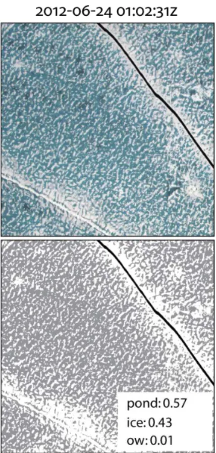
these flights are: 13 June 2012 T 22:55 Z (AP1), 22 June 2012 T 01:43 Z (AP2), 24 June 2012 T 00:08 Z (AP3), and 29 June 2012 T 14:09 Z (AP4).
C-band frequency RS-2 SAR images were acquired in fine beam quad-polarimetric (quad-pol) mode over the study site, including Parry, during the Arctic-ICE 2012 study. Each acquisition comprises a fully polarimetric (HH+VV+HV+VH and inter-channel
5
phase information) dataset, with a nominal 5.2 by 7.7 m resolution in range and az-imuth, and a 25 by 25 km image size (MDA, 2009). Despite a relatively small swath width, the low noise equivalent sigma zero (NESZ) of the quad-pol mode, nominally
−36.5±3 dB, makes it an essential tool for experimental studies of low intensity targets such as summer sea ice. In addition, our working hypothesis requires the collection
10
of scenes acquired at shallow (high) incidence angles with relatively lower backscatter levels. Of the 31 selectable beams available across the full 18◦ to 49◦incidence angle range available in fine quad-pol mode (1◦ to 2◦ width each), approximately the last 12 (39◦ to 49◦) are applicable. Extended 75 by 25 km acquisitions were made over Parry by tasking four adjacent scenes in the along-track direction and later mosaicking them.
15
Four RS-2 acquisitions over Parry were collected for this study: a descending pass prior to the onset of ponds on 12 May 2012 T 12:51 Z (R1), ascending passes during ponding on 13 June 2012 T 23:54 Z (R2) and 24 June 2012 T 00:02 Z (R4), and a de-scending pass during late ponding on 28 May 2012 T 12:51 Z (R5). A single ade-scending pass during ponding at Field on 20 June 2012 T 23:50 Z (R3) was also acquired. Each
20
of these scenes has a shallow incidence angle (41 to 44◦) and, with the exception of R3, falls within 3 h of an AP survey. R3 was a local evening overpass, with its corre-sponding survey AP2 flown approximately 24 h later.
Meteorological variables air temperature and wind speed, as well as weather obser-vations, were obtained from the WMO standard Environment Canada (EC) weather
sta-25
TCD
8, 845–885, 2014Sea ice melt pond fraction estimation –
Part 2
R. K. Scharien
Title Page
Abstract Introduction
Conclusions References
Tables Figures
◭ ◮
◭ ◮
Back Close
Full Screen / Esc
Printer-friendly Version Interactive Discussion
Discussion
P
a
per
|
D
iscussion
P
a
per
|
Discussion
P
a
per
|
Discuss
ion
P
a
per
|
at Field are used. Air temperature (±0.1◦C) and relative humidity (±0.8 %) at 2 m were sampled using a Rotronic Hygroclip 2 Probe. Surface skin temperature (±0.5◦C) was measured using an Apogee SI-111 Infrared Radiometer. Incoming longwave and short-wave radiation (±10 %) were measured using a Kipp & Zonen CNR-4 Net Radiometer. A thermistor string mounted in a melt pond provided water temperature readings at
5
0.5 cm vertical intervals.
3.2 Data processing
Each complex polarimetric RS-2 dataset was processed to a final calibrated and pro-jected product including image bands of VV, HH, and HV polarisation backscatter coef-ficients, polarisation ratios PR (VV/HH) and PRx (HV/HH), and local incidence angle.
10
Pre-processing included undersampling the raw data by a factor of 2 in range and az-imuth, in order to remove correlated adjacent pixels resulting from the SAR image for-mation process. A 5 by 5 boxcar speckle filter was applied to reduce the speckle com-ponent while preserving image statistics (Oliver and Quegan, 2004). Raw data were then converted to ground range coordinates, calibrated to sigma nought, and projected
15
to a common map projection at 12 m pixel spacing. This yielded an estimated 20 equiv-alent number of looks (ENL) at 44◦ incidence angle, based on statistics derived from user-selected homogeneous open water targets. The World Vector Shoreline (WVS), a vector data file at a nominal scale of 1 : 250 000 and provided by the NOAA National Geophysical Data Center (Soluri and Woodson, 1990), was applied to mask out land
20
within scenes.
A correction for additive noise was applied to RS-2 data before calculating PR. The metods was based on Johnsen et al. (2008), who found that the subtraction of additive noise improved calculations of PR from wind roughened ocean at high incidence an-gles. A polynomial was fitted to the range, or incidence angle (θ), dependent additive
25
TCD
8, 845–885, 2014Sea ice melt pond fraction estimation –
Part 2
R. K. Scharien
Title Page
Abstract Introduction
Conclusions References
Tables Figures
◭ ◮
◭ ◮
Back Close
Full Screen / Esc
Printer-friendly Version Interactive Discussion
Discussion
P
a
per
|
D
iscussion
P
a
per
|
Discussion
P
a
per
|
Discuss
ion
P
a
per
|
scene was determined as:
PR=10×log10
"
σ◦vv−(Aθ 4
−Bθ3+Cθ2−Dθ+F)
σ◦
hh−(Aθ4−Bθ3+Cθ2−Dθ+F)
#
, (7)
with coefficients A-F derived for each fine quad-pol (FQ) product. The additive noise was not subtracted out of the HV and HH channels before calculating the PRx since
5
we found that, as did Vachon and Wolfe (2011) when comparing PRx to ocean wind speed, this step did not improve subsequent correlations an information retrievals as it did for PR.
Digital images from AP survey lines were partitioned into scenes composed of three classes: ice, melt pond, and open water, using a decision-tree classification approach.
10
This method was based on Tschudi et al. (2001), who demonstrated the effectiveness of combining the RGB band reflectance similarities and contrasts of these features in a simple classifier. Simply, the spectral response curves of ice and open water across all RGB bands are flat, but separable in terms of magnitude, as ice is high (bright) and open water low (dark). Ponds, on the other hand, exhibit a strong contrast between red
15
and blue channels. Decision tree nodes corresponding to each survey line were con-structed in order to account for variations in ambient lighting conditions. In some cases this was done within a single survey line. After partitioning, images from high- and low-altitude survey lines were trimmed to estimated ground coverages of 900 by 900 m and 750 by 750 m, respectively, which eliminated image edges with poor radiometric
20
resolution and improved the performance of classifiers.
A classifier performance evaluation was conducted by comparing the derived rel-ative fractions of features from a set of partitioned scenes to fractions calculated by an expert using a manual approach. The manual approach involved using a K-means un-supervised classification algorithm and iteratively merging n≫3 classes to n=3
25
TCD
8, 845–885, 2014Sea ice melt pond fraction estimation –
Part 2
R. K. Scharien
Title Page
Abstract Introduction
Conclusions References
Tables Figures
◭ ◮
◭ ◮
Back Close
Full Screen / Esc
Printer-friendly Version Interactive Discussion
Discussion
P
a
per
|
D
iscussion
P
a
per
|
Discussion
P
a
per
|
Discuss
ion
P
a
per
|
Surface class statistics from AP survey lines AP1 to AP4 were matched to coincident SAR statistics from RS-2 acquisitions R2 to R5 (R1 was acquired prior to ponding) using the location information associated with each partitioned image. A 75 by 75 pixel square centred on the x, y position of a partitioned AP image was used to extract coincident SAR statistics for each co-located position along the high altitude survey
5
lines over Parry. A 60 by 60 pixel box was used for low altitude survey lines over Field. To eliminate the influence of open water on backscatter statistics, instead of ponds, partitioned AP images with>1 % open water were removed from the analysis. Finally, sample pairs were reduced by a factor of 2 to eliminate the potential for overlap and reduce the influence of spatial autocorrelation.
10
3.3 Pond fraction retrieval
Three approaches for retrieving pond fraction from calibrated RS-2 PR bands were tested. A grid composed of 7.5 by 7.5 km cells was overlaid on the study site, and collocated SAR and AP derived pond fractions corresponding to each of the four AP surveys were aggregated. This scale was chosen as it provides a good compromise
15
between the high spatial resolution RS-2 imagery and high-resolution regional scale climate models (Maslowski et al., 2011). Statistics of linear association (r2), bias, and root-mean-square error (RMSE) were used to evaluate model performances.
The first retrieval method is based on modelled incidence angle dependent functions of PR for ponds, derived from in situ C-band scatterometer observations from the same
20
study and detailed in Part 1. The following function:
PR=1.320+−0.103θ+0.004θ2, (8) describes the PR of a pure FY ice melt pond (pond fraction of 1) across the 25–60◦ incidence angle (θ) range. On the basis of an assumed ice PR of null from Part 1, combined with the assumption of linear mixing in the horizontal domain, a
look-up-25
TCD
8, 845–885, 2014Sea ice melt pond fraction estimation –
Part 2
R. K. Scharien
Title Page
Abstract Introduction
Conclusions References
Tables Figures
◭ ◮
◭ ◮
Back Close
Full Screen / Esc
Printer-friendly Version Interactive Discussion
Discussion
P
a
per
|
D
iscussion
P
a
per
|
Discussion
P
a
per
|
Discuss
ion
P
a
per
|
horizontal mixing of PR, this time with the Bragg model used for estimates of PR, as described in Sect. 2.2 and illustrated in Fig. 1. However the assumption of a null PR was also used for the Bragg based model, on the basis of the results presented in Part 1 and the documented presence of non-Bragg scattering mechanisms from the ice cover.
5
The third approach is based on cross-validation, where a sub-sample of the dataset is used to construct a predictive model, which is then applied to a set of data not used in the estimation. Full-resolution collocated data corresponding to AP2 and AP4 were used to create a linear model for the estimation of pond fraction (Fp) from PR:
Fp=0.156·PR+0.153 [dB]. (9)
10
This is not a true cross-validation approach since the model, created using full res-olution data from AP2 and AP4, was applied to aggregated samples from AP2 and AP4. Though this introduces bias in the inversion process, the approach follows that used successfully to train models for wind speed retrievals from ocean backscatter and facilitate preliminary model performance assessment (e.g., Vachon and Wolfe, 2011).
15
4 Results
4.1 Seasonal evolution of pond coverage and SAR backscatter
Average VV, HH, HV, PR, and PRxare shown along coincident average pond fractions in Table 1. Values from Parry site were derived from the area corresponding to the RS-2 image overlap region denoted in Fig. 2. Values from Field site were derived from
20
RS-TCD
8, 845–885, 2014Sea ice melt pond fraction estimation –
Part 2
R. K. Scharien
Title Page
Abstract Introduction
Conclusions References
Tables Figures
◭ ◮
◭ ◮
Back Close
Full Screen / Esc
Printer-friendly Version Interactive Discussion
Discussion
P
a
per
|
D
iscussion
P
a
per
|
Discussion
P
a
per
|
Discuss
ion
P
a
per
|
2 (and other SARs) is also possible using the data in Table 1, particularly given the shallow incidence angles used.
Baseline scene R1 was acquired on 12 May, under relatively cold (winter) conditions and several weeks prior to ponding. Backscatter at all polarisations, as well as PR, are lower than during ponding, while PRx is higher. R2 coincided with the observed
5
Ponding Stage I at Field. An average pond fraction of 0.38 during R2 is lower than expected for a Stage I peak, as previously observed in the region (Yackel et al., 2000; De Abreu et al., 2001; Scharien and Yackel, 2005). This suggests the acquisition took place during the initial stage I upturn in pond fraction. Backscatter increases relative to R1 are attributed to stronger surface scattering contributions from wind-wave
rough-10
ened ponds and wet snow, with the former caused by strong coincident wind forcing (U10=11.9 m s
−1
) from an approaching storm. A PR increase by several dB between R1 and R2 is consistent with a Bragg-like surface perturbation caused by ponds.
R3 and R4 were acquired over a four day period corresponding to Ponding Stage II at Field site, beginning one week after R2. The snow cover at Field had ablated, leaving
15
discrete pond and bare ice patches. Pond fractions (>0.5) are higher relative to R2. Backscatter at HH and HV polarisations increase relative to winter (R1) and Ponding Stage I (R2) periods. These increases are despite a significant reduction in wind stress over melt ponds compared to R2. Associated reductions in PR during Ponding Stage II point to enhanced contribution to backscatter from drained, low salinity, bare ice
20
patches. Bare ice on FY ice has been observed to have lower volumetric moisture content in its near surface layer than wet snow, which results in increased HH and VV intensities and less polarisation diversity due to volume scattering contributions (Scharien et al., 2010).
Scene R5 was acquired during the beginning of Ponding Stage III, the final stage
25
TCD
8, 845–885, 2014Sea ice melt pond fraction estimation –
Part 2
R. K. Scharien
Title Page
Abstract Introduction
Conclusions References
Tables Figures
◭ ◮
◭ ◮
Back Close
Full Screen / Esc
Printer-friendly Version Interactive Discussion
Discussion
P
a
per
|
D
iscussion
P
a
per
|
Discussion
P
a
per
|
Discuss
ion
P
a
per
|
not possible this late in the season. Based on Table 1, average backscatter and PR data are not distinguishable from Ponding Stage II.
4.2 Spatially distributed polarisation ratios and pond fractions
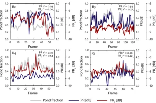
Profiles of spatially collocated polarisation ratio and pond fraction samples correspond-ing to each of the RS-2/AP survey pairs are shown in Fig. 4. Each of the AP surveys
5
comprises a wide range of pond fractions, and the entire dataset covers a 0.08–0.90 range. Though the emphasis of this study is on PR, PRxis included in Fig. 4 to provide
additional insights on the polarisation behaviour of backscatter. Coefficients of deter-mination (r2) between polarisation ratios and pond fractions in Fig. 4 are significant at
α=0.01 for each survey except for R2. Slopes of significant regression lines are all
10
positive; increases in pond fraction lead to increases in PR and PRx.
There are two noteworthy characteristics regarding the relationship between pond fraction and PR for R2 in Fig. 4. First, lack of association between variables is contrary to the Bragg model. Second, PR values are predominantly large (4–5 dB) along the survey even when pond fraction is low. From Table 1, the coincidentU10(11.9 m s−
1
) is
15
much greater than the threshold (8 m s−1) for pond surface roughness, beyond which the Bragg roughness limit is exceeded at C-band (see Scharien et al., 2014; this issue). The PR tends to unity with increasing roughness once the Bragg limit is surpassed. Considering wind stress and pond roughness are spatially variable across the scene during acquisition, contribution to the lack of association between variables is expected.
20
However, this does not explain high PR values. As it is Ponding Stage I, zones of wet snow and slush must be considered present. These features are expected to have intermediate permittivities compared to bare ice and ponds, which would cause higher PR than expected (see Sect. 2.2).
Contrasting relationships between polarisation ratios and pond fractions are
ob-25
TCD
8, 845–885, 2014Sea ice melt pond fraction estimation –
Part 2
R. K. Scharien
Title Page
Abstract Introduction
Conclusions References
Tables Figures
◭ ◮
◭ ◮
Back Close
Full Screen / Esc
Printer-friendly Version Interactive Discussion
Discussion
P
a
per
|
D
iscussion
P
a
per
|
Discussion
P
a
per
|
Discuss
ion
P
a
per
|
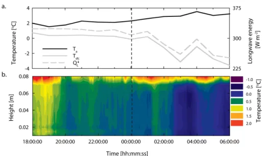
0.54). The PR range from R4 is also consistently damped, indicating a stationary pro-cess along the survey line, even in highly ponded areas. The damping of PR during R4 is examined in more detail using in situ data from the Field site over the 12 h period surrounding the acquisition (Fig. 5). Shown in Fig. 5a are meteorological variables air temperature (Ta), surface temperature (Tsfc), and downwelling longwave radiation (Q
↓ L)
5
recorded at the Field site. Figure 5b shows the temperature profile of an adjacent melt pond. Incoming longwave emissions are above 300 W m−2 and surface melt is occur-ring until 01:00Z, when longwave radiation loss and surface cooling occurs. The cooling effect on the melt pond is apparent after 02:00Z when, despite warmer air temperature, the entire pond is very close to the triple point of water. This suggests the possible
for-10
mation of a frozen surface layer on the pond, behaviour which is consistent with the clearing of the low-level stratus cloud cover that was observed to be present over the Field site during the R4 coincident AP flight at 00:00Z. The cloud layer was observed during transit to and from the Parry site, as the flight path crossed the Field site (see Fig. 2). The same cloud cover was also present over the Parry site earlier in the day, as
15
indicated by NOAA AVHRR infrared Channel 4 imagery analysed during flight planning protocols conducted at Resolute airport. Though not directly verified by data collected at Field site, earlier clearing over the Parry site likely induced a surface cooling by the time of the R4 acquisition. Surface cooling leads to less absorption and enhanced penetration of C-band energy within the drained upper layer of bare ice patches,
in-20
troducing non-Bragg, volume, scattering (Scharien et al., 2010) and a breakdown in the pond fraction – PR relationship. As suggested by Fig. 5b, cooling also leads to the possible formation of a surface ice lid on ponds and a reduction in pond PR to values resembling bare ice (see Part 1). The enhanced relationship between PRx and pond fraction during the R4 cooling event is also consistent with the formation of an ice lid on
25
pond surfaces. A positive association between PRx with ponds, seen along the survey
TCD
8, 845–885, 2014Sea ice melt pond fraction estimation –
Part 2
R. K. Scharien
Title Page
Abstract Introduction
Conclusions References
Tables Figures
◭ ◮
◭ ◮
Back Close
Full Screen / Esc
Printer-friendly Version Interactive Discussion
Discussion
P
a
per
|
D
iscussion
P
a
per
|
Discussion
P
a
per
|
Discuss
ion
P
a
per
|
The strongest coefficient of determination between pond fraction and PR (0.59) is derived from R5, despite a mixture of drained ice and melt holes indicative of Ponding Stage III, combined with remnant Ponding Stage II areas observed in partitioned AP imagery. The lowest PR (∼0 dB) during R5 also traces the minimum 0.08 pond fraction. This indicates limited detectability of pond fractions below approximately 0.10 using
5
PR across the 44–49◦ incidence angle range, behaviour which is consistent with the modelled behaviour of PR in Fig. 1.
4.3 Pond fraction retrievals
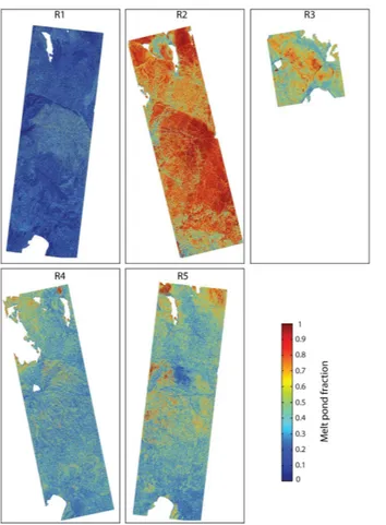
Spatial patterns of retrieved melt pond fractions, created by globally applying Eq. (8) to the PR bands from the RS-2 dataset, are shown in Fig. 6. Each of the RS-2 scenes in
10
Fig. 6 is displayed in a manner consistent with the map information provided in Fig. 2. Caution is noted regarding the interpretation of the R1 and R2. The former occurred prior to pond onset, while the latter was taken during Ponding Stage I when, as above, PR and pond fraction are not linearly associated. Nonetheless, the series clearly re-flects the onset and development of ponds. It is immediately clear that Ponding Stage I
15
is discernible from winter, despite the high wind speed and expected modulation of PR during the acquisition of R2. Considering the overlap in single polarisation backscat-ter intensities caused by variable wind stress over ponds, the PR is advantageous for identifying the onset of ponding. Scenes R3 to R5 illustrate the spatial and temporal variability in pond fraction during Ponding Stages II and III. A small polynya is also
20
visible in the top portion of the Parry site, to the north of the elongated island (Truro Island), in scenes R2, R4, and R5. The open water of the polynya appears as an area with pond fraction→1. Its growth from approximately 2–5 km width is apparent in the series. Spatial variability in pond fraction and presence of the polynya are further illus-trated by visual inspection of the R5 acquisition compared to a cloud-free Landsat-7
25
TCD
8, 845–885, 2014Sea ice melt pond fraction estimation –
Part 2
R. K. Scharien
Title Page
Abstract Introduction
Conclusions References
Tables Figures
◭ ◮
◭ ◮
Back Close
Full Screen / Esc
Printer-friendly Version Interactive Discussion
Discussion
P
a
per
|
D
iscussion
P
a
per
|
Discussion
P
a
per
|
Discuss
ion
P
a
per
|
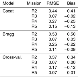
Deviations between observed and retrieved pond fractions from downscaled (7.5 km grid cell) scenes, using the three retrieval methods tested in this study, are shown in Fig. 8. Coefficients of determination between observed and cross-validation modelled pond fractions are also shown in Fig. 8. Statistics RMSE and bias for all three retrieval methods are given in Table 2. A positive bias and large RMSE is evident over R2 using
5
all three retrieval methods. This can be attributed to the contribution of wet snow/slush to higher than estimated PR in the scene (larger than expected surface permittivity). On the other hand, a negative bias and larger RMSE caused by the freezing of ponds is evident for all three retrieval methods applied to R4. Retrievals over R3 and R5 generally exhibit very small or negative bias. In cases of negative bias, it is attributed
10
to the enhanced contribution of non-Bragg scattering mechanisms from bare ice which is present during ponding stages II and III. This mechanism results in a damping of PR and pond fraction underestimations. It was only effectively accounted for by the cross-validation model, created using RS-2 data.
Model comparison is restricted to scenes R3 and R5 due to low RMSE and bias
15
associated with these acquisitions. The Cscat model generally underestimates pond fractions. As detailed in Part 1, the sampling strategy used to obtain in situ backscatter measurements and train the Cscat PR model was biased towards lower PR relative to that which are likely to occur in RS-2 data. In situ data collection strategy aimed at maximizing the impact of wind-wave roughness on backscatter parameters, in order to
20
document the limits of these parameters in relation to wind stress and wave energy. A disproportionate number of Cscat samples were collected at the upwind radar ori-entation, the only orientation at which PR was negatively correlated with wind speed. Given that data acquired at all wind speeds were used in the Cscat model, this likely contributed to a lower estimate of PR. The modified Bragg model, with the PR
contri-25
TCD
8, 845–885, 2014Sea ice melt pond fraction estimation –
Part 2
R. K. Scharien
Title Page
Abstract Introduction
Conclusions References
Tables Figures
◭ ◮
◭ ◮
Back Close
Full Screen / Esc
Printer-friendly Version Interactive Discussion
Discussion
P
a
per
|
D
iscussion
P
a
per
|
Discussion
P
a
per
|
Discuss
ion
P
a
per
|
RS-2 data to create the model. The use of RS-2 also had the benefit of input data from across the entire study domain.
5 Discussion
Several factors point to the key role of C-band SAR in coming efforts to understand and model the Arctic environment as a complex and adaptive system at increasingly finer
5
scales. First, coupling between the physical and thermodynamic evolution of snow-covered sea ice and SAR signatures is already well-established outside of the pond-ing period due to detailed in situ characterizations of physical and electromagnetic properties, and microwave interactions (e.g. Livingstone et al., 1987; Drinkwater, 1989; Barber, 2005; Perovich et al., 1998). Second, several SAR missions are either
op-10
erational or nearing launch phases, including future multi-sensor constellations ESA Sentinel-1 (Torres et al., 2012) and Radarsat Constellation Mission (Flett et al., 2009). These missions will increase the revisit frequency in polar regions to sub-daily scale while providing wide swath dual-polarisation and compact polarimetric modes. Finally, SAR sensors operating in other frequencies, e.g. L-band ALOS PalSAR-2 and X-band
15
TerraSAR-X, provide greater information content through frequency diversity. Despite its potential, the application of SAR in comprehensive EO-based sea ice process mon-itoring and modelling frameworks lags achievements at the in situ scale. This lag is due in part to uncertainties imposed by the spatial heterogeneity of sea ice, combined with variable radar parameters such as incidence angle and polarisation, when scaling to
20
the SAR scale. Continued efforts towards SAR exploitation methodologies are required (IGOS, 2007).
In this study, the well calibrated, low NESZ (−35 dB or better), and polarimetric ca-pabilities of an in situ C-band polarimetric scatterometer (see Part 1) and the satellite RS-2 operating in Fine Quad-Pol mode, facilitated the investigation of low intensity
25
TCD
8, 845–885, 2014Sea ice melt pond fraction estimation –
Part 2
R. K. Scharien
Title Page
Abstract Introduction
Conclusions References
Tables Figures
◭ ◮
◭ ◮
Back Close
Full Screen / Esc
Printer-friendly Version Interactive Discussion
Discussion
P
a
per
|
D
iscussion
P
a
per
|
Discussion
P
a
per
|
Discuss
ion
P
a
per
|
low intensity problem. The low intensity nature of the problem means results must be considered relative to the NESZ of SAR data sources. Co-polarisation (VV and HH) channels for the PR-based retrieval of pond fractions are not subject to noise floor contamination by RS-2, nor should they challenge the NESZ of conventional and fu-ture satellite SARs. Observed co-polarisation backscatter intensity values are
approxi-5
mately−20 dB or better (see Table 1). Advanced melt FY ice, irrespective of wind stress over melt ponds, does not efficiently depolarise incident microwave energy however. As such, cross-polarisation HV data, and by extension the PRx, may be subject to noise
floor contamination from SAR products outside the experimental RS-2 mode used in this study. Observed cross-polarisation backscatter intensity values are approximately
10
−28 dB or better.
Limitations to the retrieval method include the inability to quantitatively retrieve pond fractions during ponding Stage I, due to wet snow and slush contributions to PR not accounted for by Bragg model assumptions (Sect. 2.2). The high surface permittivity state and strong PR response compared to winter does mean the timing of Ponding
15
Stage I (i.e. pond onset) is identifiable in a seasonal series. The observed peak in PR from the SAR image series is closely associated with the timing of the Ponding Stage I peak in pond fraction and lowest ice albedo (Eicken et al., 2002; Perovich and Polashencki, 2012). This initial peak is expected to last only a few days as melt water easily made available by the shallow snow cover on undeformed sea ice is rapidly
20
depleted. After this the surface progresses through ponding stages II and III when, as demonstrated, PR based quantitative pond fraction retrievals are tractable.
Surface cooling events also inhibit pond fraction retrievals. The formation of an ice lid on pond surfaces occurs during surface cooling periods associated with either diurnal shortwave radiation minima or, as observed with our data, longwave radiation losses
25
TCD
8, 845–885, 2014Sea ice melt pond fraction estimation –
Part 2
R. K. Scharien
Title Page
Abstract Introduction
Conclusions References
Tables Figures
◭ ◮
◭ ◮
Back Close
Full Screen / Esc
Printer-friendly Version Interactive Discussion
Discussion
P
a
per
|
D
iscussion
P
a
per
|
Discussion
P
a
per
|
Discuss
ion
P
a
per
|
retrievals being restricted by cooling events, the resulting lack of polarization diversity and modulated PR lends itself to the identification of freeze events (i.e. surface melting state) in a seasonal series.
As defined by the frequency-dependent limiting surface roughness of the Bragg scat-tering model, sufficient wind stress over melt ponds is a source of uncertainty in pond
5
fraction retrievals. When the wind stress is high enough, nominally aU10≥8.0 m s −1
based on the findings in Part 1 of this study, the PR measured at C-band frequency is no longer independent of surface roughness. This represents a source of error in PR based models which depends on: the magnitude of the roughness (PR tends to unity with increasing roughness); and the relative fraction of rough patches contributing to
10
the backscatter within a given resolution cell. A possible solution to error induced by the roughness limit lies in the utilization of lower frequency radar than C-band. L- or P-band, which effectively increases the roughness limit by way of a largerk. However, lower frequency radar may also be more sensitive to volume scattering from bare ice, which is a non-Bragg scattering process. Further investigation is required.
15
It is worth mentioning that, despite having fully polarimetric data for this experiment, focus was placed on the information content made available by the dual-polarisation channels only. Polarimetry is undesirable for wide-area observations of features such as sea ice, since the power requirements for polarimetric sensing restricts the available swath width during acquisition compared to dual-polarisation mode (25–50 km instead
20
of several hundred km). This effectively limits the satellite revisit time over a given site.
6 Conclusions
Methods applicable to the retrieval of climatologically and biologically significant melt pond fraction on FY ice data using satellite C-band SAR were developed from a com-bination of theoretical Bragg scattering theory, in situ backscatter observations (Part
25
TCD
8, 845–885, 2014Sea ice melt pond fraction estimation –
Part 2
R. K. Scharien
Title Page
Abstract Introduction
Conclusions References
Tables Figures
◭ ◮
◭ ◮
Back Close
Full Screen / Esc
Printer-friendly Version Interactive Discussion
Discussion
P
a
per
|
D
iscussion
P
a
per
|
Discussion
P
a
per
|
Discuss
ion
P
a
per
|
relatively undeformed FY ice in the Canadian Arctic Archipelago under variable con-ditions. Model performance was evaluated using aerial photography and conventional mode skill statistics (RMSE and bias), while model intercomparisons provided valu-able insights into sources of uncertainty. The following objectives were addressed: (1) to synthesize calibrated dual-polarisation C-band frequency RADARSAT-2
backscat-5
ter statistics over undeformed FY ice during the ponding season, and (2) to evaluate a novel approach for the retrieval of melt pond fraction using the PR.
Our results suggest the C-band PR is suitable for the retrieval of FY ice melt pond fraction, with accuracies from a cross-validation model applied to downscaled 7.5 km PR samples comparable to optical methods. The approach provides a starting point
10
for quantitative pond fraction mapping without the ambiguity imposed by wind forcing on pond surfaces. Where uncertainties regarding pond fraction retrievals arise, namely Ponding Stage I when wet snow is present or during cooling events, the general PR signal is better suited to the identification of the timing of these events (e.g. in a sea-sonal time series). The PRxis potentially suited to pond fraction retrievals when ponds
15
are frozen over, though no attempt was made to model this relationship as it was an isolated event. Though our test data covered the relatively small 44 to 49◦ incidence angle range, theoretical Bragg scattering (and in situ data in Part 1) suggest that angles as low as about 40◦may be used.
In conclusion, a PR based approach provides a logical starting point for the
devel-20
opment of robust models for quantitative estimations of sea ice melt pond parameters from SAR over various ice types, and using various radar frequencies. A bottom-up testing procedure has been presented, using data of high spatial resolution compared to the research problem. Ultimately, effective pond fraction monitoring at a much larger spatial scale is required for regional scale process studies or model based
assimila-25
TCD
8, 845–885, 2014Sea ice melt pond fraction estimation –
Part 2
R. K. Scharien
Title Page
Abstract Introduction
Conclusions References
Tables Figures
◭ ◮
◭ ◮
Back Close
Full Screen / Esc
Printer-friendly Version Interactive Discussion
Discussion
P
a
per
|
D
iscussion
P
a
per
|
Discussion
P
a
per
|
Discuss
ion
P
a
per
|
Acknowledgements. This paper is dedicated to our colleague Klaus Hochheim, who lost his life in September 2013, while conducting sea ice research in the Canadian Arctic. Funding for this research was in part provided by Natural Sciences and Engineering Research Council of Canada (NSERC), the Canada Research Chairs and Canada Excellence Research Chairs programs. Randall Scharien is the recipient of a European Space Agency Changing Earth
5
Science Network postdoctoral fellowship for the period 2013–2015. Thanks to John Yackel, and his students for use of their polarimetric scatterometer. Support was provided in the form of RADARSAT-2 data by the Canadian Space Agency’s Science and Operational Applications Research (SOAR) Program, with thanks to Stephane Chalifoux. Additional RADARAT-2 scenes were provided by the Canadian Ice Service, with thanks to Tom Zagnon and Matt Arkett. We
10
acknowledge all participants of Arctic-ICE 2012, especially C. J. Mundy, lead investigator, and Megan Shields for assistance in the field. Gracious support for conducting aerial surveys was provided by ArcticNet and logistical support during the field campaign was provided by the Polar Continental Shelf Project (PCSP).
References
15
Arrigo, K. R., Perovich, D. K., Pickart, R. S., Brown, Z. W., van Dijken, G. L., Lowry, K. E., Mills, M. M., Palmer, M. A., Balch, W. M., Bahr, F., Bates, N. R., Benitez-Nelson, C., Bowler, B., Brownlee, E., Ehn, J. K., Frey, K. E., Garley, R., Laney, S. R., Lubelczyk, L., Mathis, J., Matsuoka, A., Mitchell, B. G., Moore, G. W. K., Ortega-Retuerta, E., Pal, S., Po-lashenski, C. M., Reynolds, R. A., Scheiber, B., Sosik, H. M., Stephens, M., and Swift, J. H.:
20
Massive phytoplankton blooms under Arctic sea ice, Science, 336, 1408, 2012.
Barber, D. G., Papakyriakou, T. N., LeDrew, E. F., and Shokr, M. E.: An examination of the relation between the spring period evolution of the scattering coefficient (σ◦) and radiative fluxes over landfast sea-ice, Int. J. Remote Sens., 16, 3343–3363, 1995.
Barber, D. G. and Yackel, J. J.: The physical, radiative and microwave scattering characteristics
25
of melt ponds on Arctic landfast sea ice, Int. J. Remote Sens., 20, 2069–2090, 1999. Barber, D. G.: Microwave remote sensing, sea ice and arctic climate processes, Phys. Canada,
TCD
8, 845–885, 2014Sea ice melt pond fraction estimation –
Part 2
R. K. Scharien
Title Page
Abstract Introduction
Conclusions References
Tables Figures
◭ ◮
◭ ◮
Back Close
Full Screen / Esc
Printer-friendly Version Interactive Discussion
Discussion
P
a
per
|
D
iscussion
P
a
per
|
Discussion
P
a
per
|
Discuss
ion
P
a
per
|
Comiso, J. C. and Kwok, R.: Surface and radiative characteristics of the summer Arctic sea ice cover from multisensor satellite observations, J. Geophys. Res., 101, 28397–28416, doi:10.1029/96JC02816, 1996.
De Abreu, R., Yackel, J. J., Barber, D. G., and Arkett, M.: Operational satellite sensing of Arctic first-year sea ice melt, Can. J. Remote Sens., 27, 487–501, 2001.
5
Derksen, C., J. Piwowar and LeDrew, E.: Sea-ice melt-pond fraction as determined from low level aerial photographs, Arct. Alp. Res., 29(3), 345–351, 1997.
Drinkwater, M. R.: LIMEX ’87 Ice Surface Characteristics: implications for C-Band SAR backscatter signatures, IEEE T. Geosci. Remote, 27, 501–513, doi:10.1109/TGRS.1989.35933, 1989.
10
Ehn, J. K., Mundy, C. J., Barber, D. G., Hop, H., Rossnagel, A., and Stewart, J.: Impact of hori-zontal spreading on light propagation in melt pond covered seasonal sea ice in the Canadian Arctic, J. Geophys. Res., 116, C00G02, doi:10.1029/2010JC006908, 2011.
Eicken, H., Krouse, H. R., Kadko, D., and Perovich, D. K.: Tracer studies of pathways and rates of meltwater transport through Arctic summer sea ice, J. Geophys. Res., 107, 8046,
15
doi:10.1029/2000JC000583, 2002.
Eicken, H., Grenfell, T. C., Perovich, D. K., Richter-Menge, J. A., and Frey, K.: Hy-draulic controls on summer Arctic pack ice albedo, J. Geophys. Res., 109, C08007, doi:10.1029/2003JC001989, 2004.
Fetterer, F. and Untersteiner, N.: Observations of melt ponds on Arctic sea ice, J. Geophys.
20
Res., 103, 24821–24835, 1998.
Flett, D., Crevier, Y., and Girard, R.: The RADARSAT Constellation Mission: Meeting the gov-ernment of Canada’S needs and requirements, Proceedings of the Geoscience and Remote Sensing Symposium, 2009 IEEE International, IGARSS 2009, Cape Town, South Africa, 12–17 July 2009, doi:10.1109/IGARSS.2009.5418303, 2009.
25
Flocco, D., Feltham, D. L., and Turner, A. K.: Incorporation of a physically-based melt pond scheme into the sea ice component of a climate model, J. Geophys. Res., 115, C08012, doi:10.1029/2009JC005568, 2010.
Freitag, J. and Eicken, H.: Meltwater circulation and permeability of Arctic summer sea ice derived from hydrological field experiments, Ann. Glaciol., 49, 349–358, 2003.
30
TCD
8, 845–885, 2014Sea ice melt pond fraction estimation –
Part 2
R. K. Scharien
Title Page
Abstract Introduction
Conclusions References
Tables Figures
◭ ◮
◭ ◮
Back Close
Full Screen / Esc
Printer-friendly Version Interactive Discussion
Discussion
P
a
per
|
D
iscussion
P
a
per
|
Discussion
P
a
per
|
Discuss
ion
P
a
per
|
Fung, A. K.: Microwave Scattering and Emission Models and Their Applications, Artech House, Inc., Norwood, Ma., 1994.
Golden, K. M., Ackley, S. F., and Lytle, V. I.: The percolation phase transition in sea ice, Science, 282, 2238–2241, 1998.
Hanesiak, J. M., Yackel, J. J., and Barber, D. G.: Effect of melt ponds on first-year sea ice
5
ablation-integration of RADARSAT-1 and thermodynamic modelling, Can. J. Remote Sens., 27, 433–442, 2001a.
Hanesiak, J. M., Barber, D. G., De Abreu, R. A., and Yackel, J. J.: Local and regional albedo observations of arctic first-year sea ice during melt ponding, J. Geophys. Res., 106, 1005– 1016, doi:10.1029/1999JC000068, 2001b.
10
Hajnsek, I., Pottier, E., and Cloude, S. R.: Inversion of surface parameters from polarimetric SAR, IEEE T. Geosci. Remote, 41, 727–744, 2003.
Heygster, G., Alexandrov, V., Dybkjær, G., von Hoyningen-Huene, W., Girard-Ardhuin, F., Kat-sev, I. L., Kokhanovsky, A., Lavergne, T., Malinka, A. V., Melsheimer, C., Toudal Pedersen, L., Prikhach, A. S., Saldo, R., Tonboe, R., Wiebe, H., and Zege, E. P.: Remote sensing of sea ice:
15
advances during the DAMOCLES project, The Cryosphere, 6, 1411–1434, doi:10.5194/tc-6-1411-2012, 2012.
Holland, M. M., Bailey, D. A., Briegleb, B. P., Light, B., and Hunke, E.: Improved sea ice short-wave radiation physics in ccsm4: the impact of melt ponds and aerosols on arctic sea ice, J. Climate, 25, 1413–1430, doi:10.1175/JCLI-D-11-00078.1, 2012.
20
Howell, S. E. L., Tivy, A., Yackel, J. J., and Scharien, R. K.: Application of a Sea-Winds/QuikSCAT sea ice melt algorithm for assessing melt dynamics in the Canadian Arctic Archipelago, J. Geophys. Res., 111, C07025, doi:10.1029/2005JC003193, 2006.
IGOS Cryosphere: Integrated Global Observing Strategy (IGOS) cryosphere theme report, Geneva, Switzerland, WMO/TD-No. 1405, 102 pp., 2007.
25
Inoue, J., Kosovic, B., and Curry, J. A.: Evolution of a storm-driven cloudy boundary layer in the Arctic, Bound.-Lay. Meteorol., 117, 213–230, 2005.
Inoue, J., Kikuchi, T., and Perovich, D. K.: Effect of heat transmission through melt ponds and ice on melting during summer in the Arctic Ocean, J. Geophys. Res., 113, C05020, doi:10.1029/2007JC004182, 2008.
30