Sub-grid scale representation of vegetation in global land surface schemes: implications for estimation of the terrestrial carbon sink

(1)

BGD

10, 16003–16041, 2013

Vegetation spatial representation and

the terrestrial sink

J. R. Melton and V. K. Arora

Title Page

Abstract Introduction

Conclusions References

Tables Figures

◭ ◮

Back Close

Full Screen / Esc

Printer-friendly Version Interactive Discussion

Discussion

P

a

per

|

D

iscussion

P

a

per

|

Discussion

P

a

per

|

Discuss

ion

P

a

per

|

Biogeosciences Discuss., 10, 16003–16041, 2013 www.biogeosciences-discuss.net/10/16003/2013/ doi:10.5194/bgd-10-16003-2013

Open Access

Biogeosciences Discussions

This discussion paper is/has been under review for the journal Biogeosciences (BG). Please refer to the corresponding final paper in BG if available.

Sub-grid scale representation of

vegetation in global land surface

schemes: implications for estimation of

the terrestrial carbon sink

J. R. Melton and V. K. Arora

Canadian Centre for Climate Modelling and Analysis, Environment Canada, Victoria, BC, V8W 2Y2, Canada

Received: 20 August 2013 – Accepted: 2 October 2013 – Published: 17 October 2013

Correspondence to: J. R. Melton (joe.melton.sci@gmail.com)

(2)

BGD

10, 16003–16041, 2013

Title Page

Tables Figures

◭ ◮

Back Close

Full Screen / Esc

Discussion

P

a

per

|

D

iscussion

P

a

per

|

Discussion

P

a

per

|

Discuss

ion

P

a

per

|

Abstract

Terrestrial ecosystem models commonly represent vegetation in terms of plant func-tional types (PFTs) and use their vegetation attributes in calculations of the energy and water balance and to investigate the terrestrial carbon cycle. To accomplish these tasks, two approaches for PFT spatial representation are widely used: “composite” and

5

“mosaic”. The impact of these two approaches on the global carbon balance has been investigated with the Canadian Terrestrial Ecosystem Model (CTEM v 1.2) coupled to the Canadian Land Surface Scheme (CLASS v 3.6). In the composite (single-tile)

ap-proach, the vegetation attributes of different PFTs present in a grid cell are aggregated

and used in calculations to determine the resulting physical environmental conditions

10

(soil moisture, soil temperature, etc.) that are common to all PFTs. In the mosaic (multi-tile) approach, energy and water balance calculations are performed separately for each PFT tile and each tile’s physical land surface environmental conditions evolve in-dependently. Pre-industrial equilibrium CLASS-CTEM simulations yield global totals of vegetation biomass, net primary productivity, and soil carbon that compare reasonably

15

well with observation-based estimates and differ by less than 5 % between the mosaic

and composite configurations. However, on a regional scale the two approaches can

differ by >30 %, especially in areas with high heterogeneity in land cover. Simulations

over the historical period (1959–2005) show different responses to evolving climate and

carbon dioxide concentrations from the two approaches. The cumulative global

terres-20

trial carbon sink estimated over the 1959–2005 period (excluding land use change

(LUC) effects) differs by around 5 % between the two approaches (96.3 and 101.3 Pg,

for the mosaic and composite approaches, respectively) and compares well with the

observation-based estimate of 82.2±35 Pg C over the same period. Inclusion of LUC

causes the estimates of the terrestrial C sink to differ by 15.2 Pg C (16 %) with values

25

of 95.1 and 79.9 Pg C for the mosaic and composite approaches, respectively. Spatial

differences in simulated vegetation and soil carbon and the manner in which terrestrial

(3)

substan-BGD

10, 16003–16041, 2013

Title Page

Tables Figures

◭ ◮

Back Close

Full Screen / Esc

Discussion

P

a

per

|

D

iscussion

P

a

per

|

Discussion

P

a

per

|

Discuss

ion

P

a

per

|

tially different estimate of the global land carbon sink. These results demonstrate that

the spatial representation of vegetation has an important impact on the model response

to changing climate, atmospheric CO2concentrations, and land cover.

1 Introduction

Terrestrial ecosystem (TEM) or dynamic global vegetation models (DGVM), with their

5

associated land surface schemes (LSSs), are used in Earth system models (ESMs) to

simulate the CO₂flux between the land surface and the atmosphere’s lower boundary.

An important application of TEMs and DGVMs has been to estimate the terrestrial bio-sphere’s role in the uptake of anthropogenic carbon (Le Quéré et al., 2009; Huntzinger et al., 2012) and to quantify carbon emissions due to land use change (LUC) and

10

changing climate (Arora and Boer, 2010).

Typically, LSSs use specified structural physical attributes of vegetation in their cal-culation of surface energy and water balance terms. These attributes include leaf area index, vegetation roughness height, rooting depth, fractional vegetation cover and canopy mass. When coupled to TEMs or DGVMs, vegetation is modelled as an

15

interactive component and physical attributes of vegetation are simulated as a

func-tion of driving climate and atmospheric CO2concentration ([CO2]). Coupled LSSs and

TEMs simulate fluxes of water, energy and CO2 at the atmosphere–land boundary.

Vegetation in ESMs is commonly represented in terms of broad plant functional types (PFTs). Appropriate representation of these PFTs’ spatial distribution presents a

chal-20

lenge to modellers as the area of climate model grid cells is often on the order of

100 000 km2. On these large scales, the spatial distribution of terrestrial vegetation can

be extremely heterogeneous. For example, a grid cell with a land cover that is 20 % treed and 80 % herbaceous may represent a typical savannah landscape with intermit-tent trees, or a closed-canopy forest surrounded by prairie grasslands. In reality, these

25

two landscapes represent greatly di_fferent physical and hydrological environments for

(4)

BGD

10, 16003–16041, 2013

Title Page

Tables Figures

◭ ◮

Back Close

Full Screen / Esc

Discussion

P

a

per

|

D

iscussion

P

a

per

|

Discussion

P

a

per

|

Discuss

ion

P

a

per

|

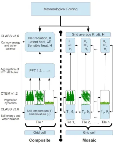
that can accurately capture the vegetation dynamics due to sub-grid scale variability without incurring excessive computational cost. In response to this requirement, the Earth System modelling community has adopted three main approaches to represent sub-grid scale vegetation variability within LSS frameworks, which are termed: (i) com-posite, (ii) mosaic, and (iii) mixed (following Li and Arora, 2012).

5

The composite approach (left column of Fig. 1) assumes that structural (as men-tioned above) and physiological attributes (e.g. stomatal conductance) of the PFTs present can be averaged across the grid cell (weighted by each PFT’s fractional cov-erage) (Verseghy, 1991; Verseghy et al., 1993; Sitch et al., 2003; Oleson et al., 2010). These grid averaged values are then used in water and energy balance calculations to

10

obtain a grid-averaged physical state of the land surface. Thus, each PFT is exposed to the same environmental variables, such as canopy temperature, soil moisture, soil temperature, and net radiation.

The mosaic representation of the land surface uses separate “tiles” for each PFT (Koster and Suarez, 1992a) (right column of Fig. 1). Each tile simulates the energy and

15

water balance based upon the interactions of the structural and physiological charac-teristics of its PFT with the driving climate, without regard to the conditions in the other tiles. As a result, the land surface state in each tile evolves independently with unique

environmental variables with corresponding different simulated energy, water and CO2

fluxes. The tiles’ fluxes are then grid-averaged prior to interaction with the lower

bound-20

ary of the atmosphere.

The mixed approach is a combination of the mosaic and composite approaches. An example of the mixed approach uses the PFT vegetation attributes for calculations of the energy and water balance for each tile, but the soil moisture and temperature are grid-averaged at the end of each time step (Sellers et al., 1986; Dickinson et al., 1993).

25

Different landscapes are better represented by one of the three approaches

(5)

BGD

10, 16003–16041, 2013

Title Page

Tables Figures

◭ ◮

Back Close

Full Screen / Esc

Discussion

P

a

per

|

D

iscussion

P

a

per

|

Discussion

P

a

per

|

Discuss

ion

P

a

per

|

to better represent landscapes with a clear distinction between PFTs such as non-overlapping cropland and closed-canopy forest. A mixed approach is usually chosen to reduce computational cost, not specifically to better represent the land surface. Com-monly, a model is run with a globally constant application of either composite or mosaic approaches, without consideration of the particular observed vegetation structure of an

5

individual grid cell.

The impact of the mosaic vs. the composite approach has been investigated with respect to the surface energy and hydrological balance (Koster and Suarez, 1992a, b; Molod and Salmun, 2002; Molod et al., 2003, 2004; Essery et al., 2003), however the impact on the carbon balance has received little attention. Li and Arora (2012)

10

analyzed site level (single grid cell) differences in simulated carbon pools and fluxes

between composite and mosaic approaches at four locations (two boreal, one temper-ate, and one tropical) with the Canadian Land Surface Scheme (CLASS) version 3.4 (Verseghy, 2009) coupled to the Canadian Terrestrial Ecosystem Model (CTEM) ver-sion 1.0 (Arora, 2003; Arora and Boer, 2005). Their analysis was designed to

gener-15

ate the largest possible difference between the composite and mosaic approaches, as

a form of sensitivity test, thus they used an idealized PFT fractional coverage of 50 % for each of the two dominant PFTs present at each location. Li and Arora (2012) reported that the primary energy fluxes were relatively insensitive to the vegetation

representa-tion with less than 5 % difference between the two approaches. However, the carbon

20

fluxes and pool sizes varied by as much as 46 % on a grid-averaged basis. Given that their simulations were intended to determine the largest influence on a site level, it

is difficult to predict how important the vegetation configuration strategy is at a global

scale, with realistic PFT fractional coverage, and under changing [CO₂], climate, and

land use. Here, we expand on the work of Li and Arora (2012) by studying the impact

25

of the manner in which sub-grid scale variability of vegetation is represented on the global terrestrial carbon balance. In addition, we investigate the model’s response to

historical changes in [CO2], climate, and land cover when using the composite and

(6)

BGD

10, 16003–16041, 2013

Title Page

Tables Figures

◭ ◮

Back Close

Full Screen / Esc

Discussion

P

a

per

|

D

iscussion

P

a

per

|

Discussion

P

a

per

|

Discuss

ion

P

a

per

|

2 Methods

2.1 Description of the CLASS and CTEM models

The CLASS-CTEM results presented here were generated from the coupling of the CLASS (v. 3.6) (Verseghy, 2012) and CTEM (v. 1.2) models. Slightly older versions of both models are currently implemented in the Canadian Centre for Climate Modelling

5

and Analysis Earth System Model (CanESM2) (Arora et al., 2011), but are used in an

off-line configuration here, driven with observation-based climate, to allow for simpler

interpretation.

CLASS operates on a half-hourly timestep driven with the atmospheric forcing data (downwelling longwave and shortwave radiation, precipitation, air pressure, specific

hu-10

midity, wind speed, and air temperature) and calculates the energy and water balances of the soil, snow, and vegetation canopy components. CLASS includes three soil lay-ers of thickness: 0.10, 0.25, and up to 3.75 m (the depth of the third layer is dependent on the grid cell soil depth to bedrock from Zobler, 1986). The temperature and liquid and frozen moisture contents are simulated for each soil layer. CLASS also simulates,

15

when snow is present, the physical characteristics (mass, density, albedo, liquid wa-ter content, and temperature) of one snow layer of a prognostically dewa-termined depth. Within a single tile, surface flux calculations are performed on tile sub-regions of (as required): (i) bare soil, (ii) vegetation covered ground, (iii) bare soil with snow cover, and (iv) vegetation over snow. CLASS performs energy and water balance calculations

20

for four PFTs: needleleaf trees, broadleaf trees, crops, and grasses (short vegetation). Each PFT has prescribed structural attributes associated with it, such as leaf area in-dex (LAI), plant height (roughness length), and rooting depth. However, when coupled to CTEM, these variables are dynamically modelled by CTEM and passed to CLASS.

CTEM simulates terrestrial ecosystem processes for nine PFTs that are directly

re-25

lated to the four CLASS PFTs. Needleleaf trees are separated into evergreen and de-ciduous; broadleaf trees into evergreen, cold deciduous, and drought/dry dede-ciduous;

(7)

BGD

10, 16003–16041, 2013

Title Page

Tables Figures

◭ ◮

Back Close

Full Screen / Esc

Discussion

P

a

per

|

D

iscussion

P

a

per

|

Discussion

P

a

per

|

Discuss

ion

P

a

per

|

simulates the processes of photosynthesis, autotrophic and heterotrophic respiration, carbon allocation, phenology, turnover, and land use change.

CTEM operates on a daily timestep (excluding the photosynthesis, leaf respiration, and canopy conductance calculations which are performed on the CLASS time step). The photosynthesis and respiration (autotrophic and heterotrophic) schemes of CTEM

5

are described in Arora (2003). Positive net primary productivity (NPP) is allocated into three live carbon pools (roots, stems, and leaves). The proportional allocation to each of these pools is influenced by the leaf phenological, light and root water status of the plant (Arora and Boer, 2005). Turnover and mortality reduces the live carbon stock and contributes to two dead carbon pools (litter and soil organic matter). The disturbance

10

(fire) module was not used in the simulations presented here.

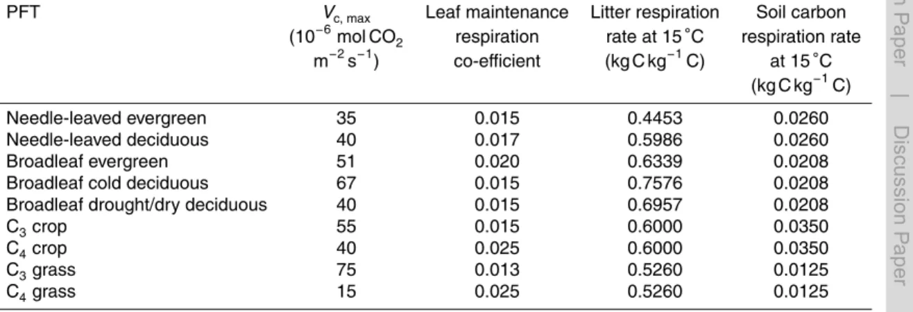
The version of CTEM used here (v 1.2) differs from the previously published version

of CTEM (v. 1.0 Arora, 2003; Arora and Boer, 2005) in: (i) its capability to perform both mosaic and composite simulations of the land surface under LUC; (ii) adjustments to

photosynthesis parameters including maximum photosynthetic rate, Vc,max, (Rogers,

15

2013); and (iii) adjustments to leaf maintenance and respiration rate parameters (see Table A1).

The vertically integrated globally-averaged carbon budget equation for the atmo-sphere can be represented as

dH_A

dt =EF−FO−FL=(EF+{ELUC})−FO−FLn (1)

20

where HA is the global atmospheric carbon burden (Pg C), FO and FL are the

at-mosphere–ocean and atmosphere–land CO₂ fluxes (Pg C yr−1) and EF is the

anthro-pogenic fossil fuel emissions (Pg C yr−1). The global net atmosphere–land CO2 flux

(FL=FLn− {ELUC}), assumed positive into the land, in CLASS-CTEM is the result of

natural CO₂ flux (F_Ln) and LUC emissions ({E_LUC}) associated with changes in land

25

cover (with the convention of positive into the atmosphere). The curly braces around

(8)

BGD

10, 16003–16041, 2013

Title Page

Tables Figures

◭ ◮

Back Close

Full Screen / Esc

Discussion

P

a

per

|

D

iscussion

P

a

per

|

Discussion

P

a

per

|

Discuss

ion

P

a

per

|

The globally-averaged land carbon budget is represented as:

FL=

dHL

dt =

dHV

dt +

dHS

dt =(GPP−RA)−RH− {ELUC}=NPP−RH− {ELUC} (2)

whereHL=HV+HS, represents the global land carbon mass, which includes the live

vegetation biomass, HV, and the dead carbon in the soil and litter pools, HS. GPP

is gross primary productivity, which yields NPP after autotrophic respiration (RA) is

5

accounted for. R_H is heterotrophic respiration and {E_LUC} represents the flux due to

LUC emissions associated with changes in land cover. When land cover is not changing

the term{ELUC}is zero andFL=FLn represents net ecosystem productivity (NEP). In

presence of LUC and other disturbances (if any), the termF_L represents net biome

productivity (NBP). Integrating Eq. (2) gives the change in total mass of land carbon

10

with respect to the cumulative land-atmosphere CO2flux (FeL):

∆HL= ∆HV+ ∆HS=FeL=

t

Z

t_o

FLdt=

t

Z

t_o

NPP dt−

t

Z

t_o

RHdt−

    

t

Z

t_o

ELUCdt

   

 (3)

e

FL=FeLn−EeLUC (4)

where the termsFeLn andEeLUC represent cumulative NEP and cumulative LUC

emis-15

sions, respectively.

In CLASS-CTEM, LUC emissions are treated in a fully interactive manner, where an increase in crop area occurs through deforestation/clearing of natural vegetation and

a reduction in theHV of natural woody or herbaceous vegetation (described in Arora

and Boer, 2010). When crop area expands into the natural vegetated areas of the grid

20

cell, as determined by the HYDE v 3.1 dataset (Hurtt et al., 2011), the biomass

re-moved,L(kg Cm−2), is divided into three components such thatL=LA+LS+LD. The

first component,LA, is combusted during clearing, or used immediately for fuel wood,

(9)

BGD

10, 16003–16041, 2013

Title Page

Tables Figures

◭ ◮

Back Close

Full Screen / Esc

Discussion

P

a

per

|

D

iscussion

P

a

per

|

Discussion

P

a

per

|

Discuss

ion

P

a

per

|

and paper products, or left in place as slash; while the final component, L_D, is used

for durable wood products. The fraction of L that each component (LA, LS or LD) is

allocated depends on whether the PFT is woody or herbaceous and the aboveground vegetation biomass density (see Table 1 in Arora and Boer, 2010). To approximate

the lifetimes of theLS and LDcomponents, these components are allocated to the

lit-5

ter and soil carbon pools, respectively. As a result the carbon that is removed from live

vegetation is emitted to the atmosphere either immediately (L_A), or with some delay

de-pending on the decomposition rate of the litter (LS) or soil C pools (LD). This approach

allows LUC impacts to influence all aspects of the terrestrial carbon budget includ-ing vegetation, litter and soil carbon pools and fluxes. The emissions of carbon due

10

to LUC are evident in the{ELUC}term as direct CO2emissions but also in increased

litter and soil C pool sizes, and subsequently, fluxes. When crop area fraction in a grid cell decreases, the fraction under natural vegetation is increased which reduces the biomass density causing the vegetation to uptake more carbon until it reaches a new equilibrium, creating the land use related carbon sink that is, for example, associated

15

with abandonment of croplands. In practice,{ELUC}is not straight-forwardly diagnosed

and, at least, two simulations are required. McGuire et al. (2001) and Arora and Boer

(2010), for example, diagnose{ELUC}according to the difference in atmosphere–land

CO2flux from simulations with and without LUC.

2.2 Model inputs

20

All CLASS-CTEM simulations were performed at the Gaussian 96×48 grid cell

reso-lution (approximately 3.75◦×3.75◦) and all inputs were interpolated to this resolution.

Climate forcing was obtained by disaggregation of the CRU-NCEP v. 4 dataset (Viovy, 2012) (1901–2010) from its native 6 hourly values to a half-hourly timestep. Shortwave radiation was diurnally interpolated based on day of year and latitude with the

maxi-25

(10)

BGD

10, 16003–16041, 2013

Title Page

Tables Figures

◭ ◮

Back Close

Full Screen / Esc

Discussion

P

a

per

|

D

iscussion

P

a

per

|

Discussion

P

a

per

|

Discuss

ion

P

a

per

|

the number of wet half-hour timesteps. The total 6 h amount was then conservatively distributed amongst the wet timesteps.

Soil texture information was adapted from Zobler (1986) with soil texture within each grid cell kept the same for both composite and mosaic configurations. For the historical

1850–2005 period, the [CO2] is based on phase 5 of the Coupled Model

Intercompar-5

ison Project (CMIP5) dataset (Meinshausen et al., 2011). The changes in fractional coverage of non-crop PFTs are inferred based on the changes in crop area following the HYDE v 3.1 dataset (Hurtt et al., 2011) using the linear interpolation approach of Arora and Boer (2010). The resulting transient land cover for the period 1850–2005 has also been used in CanESM2’s simulations for CMIP5 (Arora et al., 2011).

10

2.3 Simulations

Results from five simulations are presented here for both the mosaic and composite ap-proaches (Table 1). The pre-industrial equilibrium spin-ups, corresponding to the year 1861, form the starting point for each of the four transient historical runs (1861–2005),

which were driven with different combinations of CO2, climate and LUC forcings. These

15

include: (i) evolving climate with fixed 1861 land cover and [CO2] (“Climate only”), (ii)

evolving climate and CO₂ with fixed 1861 land cover (“Climate+CO₂”), (iii) evolving

climate and land cover with fixed 1861 [CO₂] (“Climate₊LUC”), and (iv) evolving

cli-mate, [CO2], and land cover (“Climate+CO2+LUC”). Since the CRU-NCEP climate

data does not extend back past 1901, for 1861–1900 we use the climate of 1901–

20

1940. We also do not extend past 2005 as that is the last year in the HYDE v. 3 dataset as used in the CMIP5 simulations. For most of the results presented here, we limit our analysis to the 1959–2005 period for ease of comparison with the results of other dy-namic vegetation models and the estimated terrestrial C land sink as summarized in Le Quéré et al. (2013).

25

The pre-industrial equilibrium run used a constant globally uniform [CO2] of

(11)

BGD

10, 16003–16041, 2013

Title Page

Tables Figures

◭ ◮

Back Close

Full Screen / Esc

Discussion

P

a

per

|

D

iscussion

P

a

per

|

Discussion

P

a

per

|

Discuss

ion

P

a

per

|

1861 and climate from 1901–1940 cycled over repeatedly until model pools reached equilibrium (Table 1). Equilibrium is assumed to have been attained when net

ecosys-tem productivity,FLn, varies less than 0.001 % of NPP averaged across the final 40 yr

of the simulation. Composite and mosaic simulations were spun up separately.

3 Results

5

3.1 Comparison to observationally-based datasets

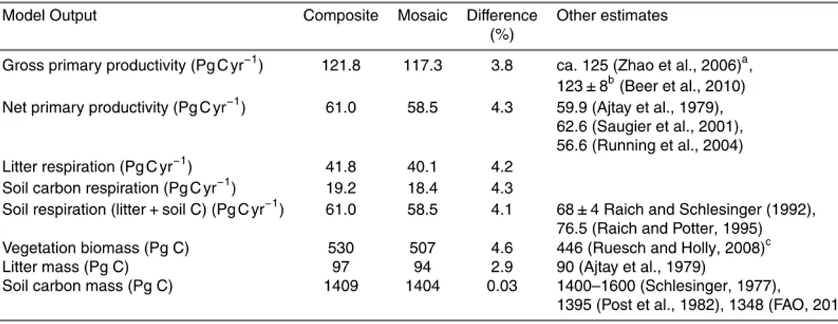
The pre-industrial equilibrium simulations’ global totals for primary model outputs are listed in Table 2. Both the composite and mosaic approaches simulate global totals of GPP, NPP, soil respiration, vegetation biomass, litter mass, and soil carbon in line with

observation-based estimates (Table 2). For these global sums, the difference between

10

the composite vs. mosaic approach is minor (maximum 4.6 % across the primary model outputs). Overall, the composite approach yields higher productivity and respiratory fluxes, and higher vegetation and soil carbon pools, than the mosaic approach.

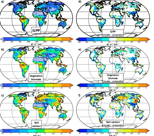
Zonally, CLASS-CTEM reproduces reasonable patterns of GPP, vegetation biomass and soil carbon as compared to observation-based datasets for contemporary

condi-15

tions (Fig. 2). While the CLASS-CTEM results (“Climate+CO2+LUC”) in Fig. 2 include

the influence of LUC, they do not include biomass burning as a disturbance agent, which would influence the model results in some fire-prone regions. An observation-based GPP estimate from Beer et al. (2010) is used for comparison with CLASS-CTEM outputs. Beer et al. (2010) analyze the ground-based carbon flux tower observations

20

from ca. 250 stations using diagnostic models to extrapolate them to the global scale for the 1998–2005 period. Mean zonal GPP simulated by CLASS-CTEM displays the same general pattern as the Beer et al. (2010) dataset (Fig. 2a). CLASS-CTEM

simu-lates slightly higher values at the equator and below about 35◦S than Beer et al. (2010),

but slightly lower values for latitudes>45◦N and around 15◦N. The composite and

(12)

BGD

10, 16003–16041, 2013

Title Page

Tables Figures

◭ ◮

Back Close

Full Screen / Esc

Discussion

P

a

per

|

D

iscussion

P

a

per

|

Discussion

P

a

per

|

Discuss

ion

P

a

per

|

saic CLASS-CTEM zonal GPP shows only small di_fferences around 10◦N–30◦N and

around 20◦S–40◦S, with a higher GPP simulated when using the composite approach.

For zonally-averaged vegetation biomass (Fig. 2b), CLASS-CTEM simulates an equatorial peak in vegetation biomass slightly higher than the Ruesch and Holly (2008) dataset for both approaches. This dataset is based upon remotely sensed vegetation

5

cover (Global Land Cover 2000 Project, GLC2000) and IPCC methods for

estimat-ing carbon stocks at the national level. For latitudes >30◦N and <30◦S,

CLASS-CTEM simulates a higher mean vegetation biomass than Ruesch and Holly (2008)

with a prominent peak around 45◦S. The mosaic and composite approaches differ

lit-tle in zonal mean vegetation biomass except for small di_fferences around 10◦N–30◦N

10

where the composite approach has a noticeably higher value. The methods employed to create the Ruesch and Holly (2008) dataset are not directly linked to ground-based measures of carbon stocks and have also not been validated with field data. The dataset may underestimate vegetation biomass at high latitudes. For example, its veg-etation biomass values are less than half that of inventory based estimates for British

15

Columbia, Canada (Peng et al., 2013).

The CLASS-CTEM mosaic and composite approaches’ zonally averaged soil carbon is compared to the Harmonized World Soils Dataset (HWSD) (FAO, 2012) in Fig. 2c. The HWSD dataset is more reliable for Southern and Eastern Africa, Latin America and the Caribbean, and Central and Eastern Europe. It is considered less reliable for

20

North America, Australia, areas of West Africa and South Asia (FAO, 2012). While the zonal distribution of simulated soil carbon is broadly similar to observation-based

HWSD estimate, some differences remain. Between 45◦N–70◦N, CLASS-CTEM

sim-ulates appreciably less soil carbon than the HWSD, with values around the equator,

15◦N, and below 50◦S also lower (below 50◦S has little landmass thus the large value

25

in the HWSD dataset is likely the result of high values in relatively few grid cells). Some

of the difference between CLASS-CTEM and HWSD is due to the fact that peatlands,

which contain high amounts of organic carbon, are not presently simulated by

(13)

sim-BGD

10, 16003–16041, 2013

Title Page

Tables Figures

◭ ◮

Back Close

Full Screen / Esc

Discussion

P

a

per

|

D

iscussion

P

a

per

|

Discussion

P

a

per

|

Discuss

ion

P

a

per

|

ulates appreciably more soil carbon around 30◦N–50◦N and in most of the Southern

Hemisphere.

3.2 Spatial di_fferences between the approaches

Figure 3a–c shows the spatial distribution of simulated GPP, vegetation biomass and soil C mass from the pre-industrial equilibrium simulation when using the mosaic

ap-5

proach. The corresponding spatial differences between the composite and mosaic

approaches are shown in Fig. 3d–f. The major regions of difference for vegetation

biomass and GPP, which can be>30 %, include southeast Asia, the Pampas region

in Argentina, the west coast of North America, southeast US, northern mainland Eu-rope, and Mexico (Fig. 3d and e). In each of those regions, the composite simulation

10

calculates higher GPP and vegetation biomass. The mosaic approach yields higher GPP and vegetation biomass for some regions, such as eastern Canada, China, the

central US, and Patagonia, however the magnitude of the difference is smaller than for

the regions where composite simulates larger values. The simulated soil carbon mass

differences between the mosaic and composite runs (Fig. 3f) follows a similar pattern

15

to the differences in vegetation biomass with southeast Asia, the Pampas of Argentina,

the west coast of North America, northwest mainland Europe, and southeast Australia simulated to have higher soil carbon mass in the simulation using the composite ap-proach. Some other regions show contrasting patterns between vegetation biomass and soil carbon, including the southeast US, the Chilean coast, the Baltics, and

west-20

ern Russia, although the differences are relatively small.

3.3 Transient historical simulations

Four simulations were performed to investigate the effect of using the composite

ver-sus mosaic approach on the historical terrestrial carbon budget. The simulations were

driven with different combinations of CO2, climate and LUC forcings (as described in

(14)

BGD

10, 16003–16041, 2013

Title Page

Tables Figures

◭ ◮

Back Close

Full Screen / Esc

Discussion

P

a

per

|

D

iscussion

P

a

per

|

Discussion

P

a

per

|

Discuss

ion

P

a

per

|

Sect. 2.3 and Table 1): (i) Climate only, (ii) Climate+CO₂, (iii) Climate+LUC, and (iv)

Climate+LUC+CO2.

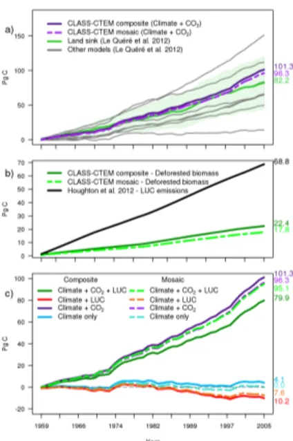
In Fig. 4a, simulatedFeLfrom the Climate+CO2simulation (using both the composite

and mosaic approaches) is compared to an observation-based estimate and simula-tions from eight other TEMs/DGVMs (as presented in Le Quéré et al., 2013). Since

5

the Climate₊CO₂simulation does not include land use change, thusFeL=FeLn, which

essentially represents cumulative NEP. Fe_Ln is also referred to as the residual

terres-trial C sink whose value can be determined as the residual of other observation-based

terms in Eq. (1). The observation-based estimate ofFeLn from Le Quéré et al. (2013)

in Fig. 4a is their estimate of the residual terrestrial C sink after accounting for

fos-10

sil fuel and LUC emissions, change in atmospheric C burden and the ocean C sink. This does not include gross land C sinks directly resulting from LUC (e.g. regrowth of

vegetation), but does include the influence of CO₂fertilization, nitrogen deposition, and

other climate change effects such as changes to growing season length. SimulatedFeLn,

over the 1959–2005 period, does not di_ffer greatly between the mosaic (96.3 Pg C) and

15

composite (101.3 Pg C) approaches while comparing reasonably with the

observation-based estimate (82.2±35 Pg C) from Le Quéré et al. (2013) and lying within the range

of other TEMs/DGVMs.

Introducing changes in land cover imply that the termELUCis not zero and the

cumu-lative atmosphere–land CO2 flux is reduced (FeL=FeLn−EeLUC) to yield the cumulative

20

NBP. Note that our definition of NBP, in the context of CLASS-CTEM, does not include

the effect of disturbance agents such as fire, insects, management-climate interactions,

and nitrogen dynamics. Figure 4b shows the cumulative deforested biomass in the

Cli-mate+LUC+CO2simulation when using the composite and mosaic approaches over

the 1959–2005 period. The deforested biomass is somewhat higher in the

compos-25

(15)

ap-BGD

10, 16003–16041, 2013

Title Page

Tables Figures

◭ ◮

Back Close

Full Screen / Esc

Discussion

P

a

per

|

D

iscussion

P

a

per

|

Discussion

P

a

per

|

Discuss

ion

P

a

per

|

proach where changes in cropland and pasture area, wood harvesting and logging, and shifting cultivation are accounted for via transfer to pools with prescribed turnover rates.

Figure 4c compares cumulative atmosphere–land CO2flux FeL from all four

simula-tions when using both the mosaic and composite approaches. Over the 1959–2005

5

period, the Climate only simulation shows no strong net emission, or uptake, of car-bon by the land surface when using the mosaic approach (0.0 Pg C) and only a slight carbon uptake by the land surface when the composite approach is used (4.1 Pg C).

The Climate₊LUC simulations give a net land C source with mosaic and

compos-ite cumulative NBP values of 7.6 Pg C and 10.2 Pg C, respectively. Climate+CO2

10

simulations show a large terrestrial carbon uptake of 96.3 Pg C and 101.3 Pg C for mosaic and composite approaches, respectively, as also seen in Fig. 4a. Finally,

the Climate+LUC+CO2 simulation reduces the estimated terrestrial C sink slightly

to 95.1 Pg C (1 % reduction compared to the Climate+CO2 simulation) when

us-ing the mosaic approach, but a much stronger reduction is seen in the

compos-15

ite approach (79.9 Pg C; 21 % reduction compared to the Climate+CO2 simulation)

at the end of the 1959–2005 period. Overall, the difference between the composite

and mosaic approaches, for global carbon uptake, is most pronounced for the

Cli-mate+CO2+LUC simulation. Diagnosing cumulative LUC emissions, EeLUC, as the

difference between cumulative atmosphere–land CO2flux between the Climate+CO2

20

and Climate₊CO₂₊LUC simulations, in a manner similar to McGuire et al. (2001) and

Arora and Boer (2010) we obtainEe_LUCas 21.4 Pg C and 1.2 Pg C for the composite and

mosaic approaches, respectively.

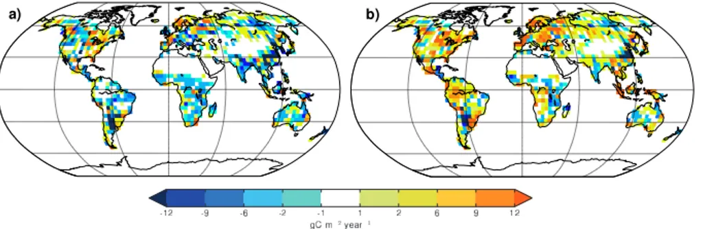
Geographical distributions of the difference in atmosphere–land CO2 flux (FL)

aver-aged over the period 1959–2005 between the mosaic and composite approaches are

25

shown in Fig. 5 from the Climate+CO2(panel a) and Climate+CO2+LUC (panel b)

simulations. For the Climate+CO2simulation (Fig. 5a) the difference between the

(16)

BGD

10, 16003–16041, 2013

Title Page

Tables Figures

◭ ◮

Back Close

Full Screen / Esc

Discussion

P

a

per

|

D

iscussion

P

a

per

|

Discussion

P

a

per

|

Discuss

ion

P

a

per

|

the composite approach simulates a larger C sink. Although there are some regions (including the American midwest and parts of Scandinavia and western Russia) where

the mosaic approach yields a larger C sink, in the Climate+CO2 simulation, for most

regions the sink is larger when the composite approach is used. When LUC is consid-ered (Fig. 5b) the general pattern shifts to larger uptake of C in the mosaic approach

5

rather than in the composite approach (as in Fig. 5a), but the regions with the largest

difference between the composite and mosaic approaches remain the same (e.g. parts

of Argentina, southern China, and Mexico).

4 Discussion

CLASS-CTEM produces estimates of GPP, NPP, soil respiration, vegetation biomass,

10

and litter and soil carbon mass that compare reasonably well with observational esti-mates (Fig. 2 and Table 2) for both mosaic and composite configurations. The impor-tance of the composite or mosaic approach in an equilibrium simulation on a global

scale is minor with the difference consistently<5 % for several model variables.

How-ever, the spatial differences are much greater and appear to be consistent across

dif-15

ferent model variables including GPP, vegetation biomass and soil C mass (Fig. 3).

The differences between the mosaic and composite approaches are related to the

rep-resentation of sub-grid scale variability of vegetation and the consequent manner in

which grid-averaged energy and water balances evolve, leading to differences in net

radiation absorbed by vegetation, soil temperature and moisture, etc. as illustrated in

20

Li and Arora (2012). To aid interpretation of the differences between simulations using

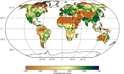
the mosaic and composite approaches, we derive a heterogeneity (H) index as follows:

H=1−

1

N N

P

i=1

(fi−f¯)

2

¯

(17)

BGD

10, 16003–16041, 2013

Title Page

Tables Figures

◭ ◮

Back Close

Full Screen / Esc

Discussion

P

a

per

|

D

iscussion

P

a

per

|

Discussion

P

a

per

|

Discuss

ion

P

a

per

|

wheref_i,i=1,. . .,N is the fractional coverage of a PFT as a function of the total

veg-etated fraction of the grid cell. For example, if one PFT covers 60 % of a grid cell and a second PFT covers 20 % with bare ground for the rest of the grid cell (20 %) then

the values off_i are 0.75 and 0.25 for each, respectively. ¯f is the mean PFT fractional

coverage.Nis the number of PFTs (nine in CTEM). Regions of high PFT heterogeneity

5

(grid cells with many different PFTs) have H index values close to 1 while regions of

low PFT heterogeneity (grid cells with few PFTs present) are close to 0. Eq. (5) yields

anH value of 1 if a grid cell contains N PFTs and each occupies (1/N)th fraction of

the grid cell, indicating maximum possible heterogeneity, and a value of 0 if an entire grid cell is occupied with only a single PFT. It is expected that the simulations using

10

the composite and mosaic approaches will di_ffer more in regions of high heterogeneity

and less in areas ofH index closer to 0. The global distribution of theH index based

on 1861 land cover used here with crop fraction based on the HYDE v 3.1 dataset is

shown in Fig. 6. Areas of highH index include parts of Mexico, Europe, China, India,

eastern Australia, and the eastern US. Areas of lowHindex include arid regions, such

15

as central Australia; tropical regions, such as the Amazon; and the high north. Areas

of lowH index are thus regions with the vegetation biomass spread across very few

PFTs.

Comparing the H index (Fig. 6) to spatial differences between composite and

mo-saic simulations for the equilibrium simulation (Fig. 3) demonstrates a strong linkage

20

as anticipated. Areas of highH index generally have higher GPP, vegetation biomass

and soil carbon mass when the composite approach is used. Regions with moderate

H index values are not strongly biased towards either approach. Areas of low H are

generally similar in simulations using the composite and mosaic approaches, as

ex-pected. The differences between the model configurations evident in Fig. 3 are related

25

to di_fferences in the energy and water balances calculations in the two approaches,

as noted by Li and Arora (2012). Li and Arora (2012) observed differences in net

radi-ation flux (due to albedo differences); latent and sensible heat flux; and soil moisture

(18)

BGD

10, 16003–16041, 2013

Title Page

Tables Figures

◭ ◮

Back Close

Full Screen / Esc

Discussion

P

a

per

|

D

iscussion

P

a

per

|

Discussion

P

a

per

|

Discuss

ion

P

a

per

|

sites, when driven with identical climate. Net radiation and soil moisture directly influ-ence photosynthesis and simulated canopy and soil temperatures influinflu-ence respiratory fluxes.

Across the historical period (1959–2005) in the Climate+CO₂ simulation,

CLASS-CTEM simulates a global terrestrial C sink in-line with other model estimates and the

5

land sink estimated by Le Quéré et al. (2013) (Fig. 5a). The difference between the

global total mosaic and composite approaches estimated land C sink is small (ca. 5 %)

(Fig. 4a), but can be large for different regions. The areas of largest disagreement

for the estimated terrestrial C sink (without LUC effects) between the composite and

mosaic simulations are generally regions of highHindex, with a few notable exceptions

10

such as areas in the US Prairies (compare Figs. 5a and 6).

Incorporation of LUC has a marked impact on the difference in the estimated global

terrestrial C sink (cumulative NBP; Fig. 4c) between the simulations using the mosaic and composite configurations. Our simulated deforested biomass across both config-urations is lower than the “book-keeping” estimate of Houghton et al. (2012) since we

15

take into account only the changes in crop area, i.e. the effect of increasing pasture

area over the historical period is not considered, and we do not account for wood har-vesting and logging, shifting cultivation, and urbanization. Land use change emissions

are extremely difficult to quantify, with at least a±50 % uncertainty (Ramankutty et al.,

2006), and LUC is represented in TEMs and DGVMs using a range of parametrizations

20

(e.g. see Brovkin et al., 2013).

LUC causes the estimated terrestrial C sink to drop by 21.4 Pg C when using the composite approach, as would be generally expected since LUC releases carbon from burning and decomposition of the deforested biomass. In the mosaic configuration, however, LUC causes the terrestrial sink to drop by only 1.2 Pg C (Fig. 4c; compare

25

Climate₊CO₂ vs. Climate₊CO₂ ₊LUC), yielding a 16 % di_fference in the estimated

global terrestrial sink, over the 1959–2005 period, between the two approaches. The

larger effect of LUC on the composite configuration’s cumulative NBP, over the mosaic,

(19)

BGD

10, 16003–16041, 2013

Title Page

Tables Figures

◭ ◮

Back Close

Full Screen / Esc

Discussion

P

a

per

|

D

iscussion

P

a

per

|

Discussion

P

a

per

|

Discuss

ion

P

a

per

|

The LUC scheme in CLASS-CTEM removes natural vegetation when crop area in-creases. When LUC occurs, the amount of C that is burned or transferred to the litter and soil C pools depends on the vegetation biomass of the PFT that occupies that frac-tion of grid cell that is encroached upon at the time of LUC. In CLASS-CTEM, crops have higher productivity than the natural vegetation they replace. However, crop

pro-5

ductivity also depends on whether the mosaic or composite configuration is used. To

interpret the differences between the mosaic and composite approaches, in the

simula-tion with LUC, we define an addisimula-tional measure that quantifies changes in crop fracsimula-tion

in a grid cell. The mean annual relative change in crop fraction, ¯RC, is calculated as:

¯

RC=

XT

t=2| fc(t)−fc(t−1)|

T−1 ×100 % (6)

10

wheref_c(t) is the fractional crop area for a grid cell at timetandT is 47 yr, i.e. the period

1959–2005. The ¯RCover the 1959–2005 period is shown in Fig. 7. The major areas of

LUC include the US midwest and prairie region of Canada, eastern Europe, western Russia, and parts of northern India, China, southeast Australia and Argentina. While

theHindex is arguably sufficient for interpreting the differences in the simulations with

15

mosaic and composite configurations evident in Fig. 5a (Climate+CO2), i.e. in

simu-lations without LUC, the contribution of both heterogeneity (Fig. 6) and LUC (Fig. 7)

cause the differences in cumulativeFeL between the composite and mosaic

configura-tions visible in Fig. 5b (Climate+CO2+LUC). In general, areas of highH index have

greater visible differences between the mosaic and composite approaches, and these

20

are then exaggerated by LUC processes, since the effect of LUC is influenced by the

manner in which vegetation is represented.

To illustrate how the effect of LUC depends on representation of vegetation (using the

composite or the mosaic approach) we show results from a grid cell that is

represen-tative of regions with highH index and high LUC (Fig. 8) over the simulated historical

25

period (1861–2005). Grid cells with a highH index demonstrate larger differences

(20)

BGD

10, 16003–16041, 2013

Title Page

Tables Figures

◭ ◮

Back Close

Full Screen / Esc

Discussion

P

a

per

|

D

iscussion

P

a

per

|

Discussion

P

a

per

|

Discuss

ion

P

a

per

|

accentuates differences between the model approaches. In the grid cell chosen for this

purpose (50.10◦N and 46.88◦E, near Volgograd, Russia), there is a large LUC, as

ev-ident in a doubling of C3 crop fraction and a resulting reduction in the tree fraction,

between 1861 and 2005 as seen in Fig. 8a. For this grid cell, the composite approach simulates a larger vegetation biomass in 1860 in the pre-industrial equilibrium

sim-5

ulation (Fig. 8b) due to a higher grid-averaged NPP (Fig. 8c). As the C3 crop fraction

expands, the fraction of other PFTs is reduced and the grid average vegetation biomass for both mosaic and composite simulations decreases (Fig. 8b). The amount of carbon

deforested from the live vegetation pools differs between the composite and mosaic

simulations (Fig. 8d), since the amount of biomass removed depends on the amount

10

that is present, but overall with the same pattern. That is, despite the same changes in fractional coverage of PFTs between the approaches, the amount of natural vegetation

deforested differs. Since the deforested biomass is larger in the composite approach,

over the historical period, it simulates a steeper decline in grid-averaged vegetation biomass (Fig. 8b). The soil C pools are initially smaller for the composite configuration

15

(Fig. 8e) due to higher soil temperatures (not shown) despite higher litter inputs asso-ciated with higher initial productivity (Fig. 8c) in the composite compared to the mosaic approach. As carbon is transferred to the soil C pool by LUC, the two configurations diverge further. Soil C mass decreases in the composite approach and increases in the mosaic approach. The decline in soil C mass in the composite approach is due

20

to the faster rate of shrinking vegetation biomass (Fig. 8b) and diminishing amounts of biomass transferred, as well as warmer soils in the composite approach promoting faster decomposition. As crop area expands the grid-averaged NPP in the mosaic con-figuration approaches that of the composite (Fig. 8c) due to a faster rate of increase of crop productivity (not shown). Recall that in the mosaic configuration crops are grown

25

in their individual tile, while in the composite approach they share the same physi-cal land surface climate, including soil moisture, as other PFTs. The net result is that

the trajectory of the cumulative atmosphere–land CO2flux (FeL) differs greatly between

(21)

com-BGD

10, 16003–16041, 2013

Title Page

Tables Figures

◭ ◮

Back Close

Full Screen / Esc

Discussion

P

a

per

|

D

iscussion

P

a

per

|

Discussion

P

a

per

|

Discuss

ion

P

a

per

|

posite approach yields a net source of C, while the mosaic approach simulates the grid

cell to be a C sink. The differences in simulated energy and water balances between

the two approaches act in a manner such that in the mosaic approach the increasing productivity associated with increasing crop area overcomes the resulting emissions

from burning and decomposition of deforested biomass. The different responses of

5

grid-averaged carbon balance in this grid cell illustrate how the net effect of global LUC

can be quite different for the two approaches.

The strong influence of the model vegetation spatial configuration has implications for model estimates of carbon emissions due to LUC. Estimates of the total LUC emis-sions range from 72 Pg C to 115.2 Pg C across the 1920–1999 period (Houghton et al.,

10

2012). The CLASS-CTEM LUC parametrization gives a global LUC emissions esti-mate that is on the low-end of other models. Arora and Boer (2010) estiesti-mate 73.6 Pg C across the same time period using CLASS v. 2.7 with CTEM v. 1.0 in a composite configuration coupled into CanESM1 (Arora et al., 2009).

Our results suggest that the use of the mosaic configuration will yield an even lower

15

estimate of LUC emissions. The sensitivity of modelled LUC emissions to spatial rep-resentation of vegetation makes the task of modelling LUC emissions in TEMs and

DGVMs somewhat more difficult, given the already uncertain LUC emissions and the

wide variety of parametrizations using which LUC emissions are modelled. It is difficult

to definitively conclude which approach is better, mosaic or composite, and these

re-20

sults only illustrate that model architecture can have a significant influence on modelled LUC emissions.

5 Conclusions

Dynamic vegetation models must represent the sub-grid heterogeneity of terrestrial

vegetation in a manner that is computationally efficient and best captures vegetation

25

(22)

BGD

10, 16003–16041, 2013

Title Page

Tables Figures

◭ ◮

Back Close

Full Screen / Esc

Discussion

P

a

per

|

D

iscussion

P

a

per

|

Discussion

P

a

per

|

Discuss

ion

P

a

per

|

investigated previously. Here, we have used global simulations of the terrestrial carbon

budget over the historical period to illustrate the effect of using the composite versus

the mosaic approach.

In our equilibrium spin-up simulations using CLASS-CTEM, in either the

compos-ite or mosaic configurations, we see no large differences in the global sums of model

5

variables like vegetation biomass, GPP, NPP, soil C and litter mass between the two

approaches (<5 %). However, spatially, the differences between the two approaches

can be large for these model variables (>30 %). These differences are most apparent

in regions with high heterogeneity of land cover (with regard to the number of PFTs) where the mosaic and composite representations are less comparable. In transient

10

simulations, the mosaic and composite approaches respond di_fferently to changing

cli-mate and CO2. The difference in cumulative atmosphere–land CO2 flux is 5 Pg C, or

around 5 %, over the 1959–2005 period in Climate+CO2 simulations. When LUC is

accounted for, the di_fference between the cumulative atmosphere–land CO₂flux in the

simulations using the composite and mosaic configuration increases to 15.2 Pg C (or

15

around 16 %) and spatial differences increase further. The diagnosed LUC emissions,

calculated as the di_fference between cumulative atmosphere–land CO₂flux from

sim-ulations with and without LUC, are 21.4 Pg C and 1.2 Pg C for the composite and mo-saic approaches, respectively. These estimates are much lower than Houghton et al. (2012) since we do not account for changes in pasture area, wood harvesting, or

shift-20

ing cultivation. CLASS-CTEM also treats crop PFTs explicitly, rather than using grass PFTs in place of crops as is common among most ESMs (Brovkin et al., 2013). In CLASS-CTEM, the higher productivity of crops contributes to the higher rate of NPP

as croplands expand and as CO2 increases and this acts to further lower estimated

LUC emissions. Irrespective of comparison with the Houghton et al. (2012) estimate,

25

our results show that the di_fference between the two approaches of representing

sub-grid heterogeneity of vegetation is largest when LUC is accounted for in conjunction

with increasing CO2 and changing climate. The CLASS-CTEM LUC scheme is

(23)

BGD

10, 16003–16041, 2013

Title Page

Tables Figures

◭ ◮

Back Close

Full Screen / Esc

Discussion

P

a

per

|

D

iscussion

P

a

per

|

Discussion

P

a

per

|

Discuss

ion

P

a

per

|

water balances evolve differently in composite vs. mosaic configuration (as noted in

Li and Arora, 2012), the same location can have a completely different evolution of

its vegetation depending on the model configuration. This divergent evolution between

model configurations leads to the large spatial differences in vegetation biomass and,

if LUC is accounted for, in the amount of natural vegetation mass that is deforested.

5

An important application of dynamic vegetation models has been to estimate the size of the terrestrial land sink (Huntzinger et al., 2012; Le Quéré et al., 2013) and to estimate the contribution of LUC emissions to the global C budget (McGuire et al., 2001). Our results indicate that any estimates of LUC emissions obtained from dynamic vegetation models can be potentially influenced by the choice of sub-grid scale spatial

10

representation of the land surface. Since it is not readily apparent which representation (mosaic or composite) is more appropriate, care should be taken in interpreting model estimates of LUC emissions.

Acknowledgements. We thank Simon Griffith for his assistance in preparing the CRU-NCEP

climate files. Nadja Steiner, Diana Verseghy, and Paul Bartlett provided helpful comments

15

on an earlier version of the manuscript. J. R. Melton was supported by an NSERC Visiting Postdoctoral Fellowship.

The works published in this journal are distributed under the Creative Commons Attribu-tion 3.0 License. This license does not affect the Crown copyright work, which is re-usable

20

under the Open Government Licence (OGL). The Creative Commons Attribution 3.0 License and the OGL are interoperable and do not conflict with, reduce or limit each other.

References

25

(24)

BGD

10, 16003–16041, 2013

Title Page

Tables Figures

◭ ◮

Back Close

Full Screen / Esc

Discussion

P

a

per

|

D

iscussion

P

a

per

|

Discussion

P

a

per

|

Discuss

ion

P

a

per

|

Arora, V.: Modeling vegetation as a dynamic component in soil-vegetation-atmosphere transfer schemes and hydrological models, Rev. Geophys., 40, 3-1–3-26, doi:10.1029/2001RG000103, 2002.

Arora, V. K.: Simulating energy and carbon fluxes over winter wheat using coupled land surface and terrestrial ecosystem models, Agr. Forest Meteorol., 118, 21–47,

doi:10.1016/S0168-5

1923(03)00073-X, 2003. 16007, 16009

Arora, V. K. and Boer, G. J.: A parameterization of leaf phenology for the terrestrial ecosys-tem component of climate models, Glob. Change Biol., 11, 39–59, doi:10.1111/j.1365-2486.2004.00890.x, 2005. 16007, 16009, 16033

Arora, V. K. and Boer, G. J.: Uncertainties in the 20th century carbon budget

associ-10

ated with land use change, Glob. Change Biol., 16, 3327–3348, doi:10.1111/j.1365-2486.2010.02202.x, 2010. 16005, 16010, 16011, 16012, 16017, 16023

Arora, V. K., Boer, G. J., Christian, J. R., Curry, C. L., Denman, K. L., Zahariev, K., Flato, G. M., Scinocca, J. F., Merryfield, W. J., and Lee, W. G.: The effect of terrestrial phtosynthesis down regulation on the twentieth-century carbon budget simulated with the CCCma Earth System

15

Model, J. Climate, 22, 6066–6088, doi:10.1175/2009JCLI3037.1, 2009. 16023

Arora, V. K., Scinocca, J. F., Boer, G. J., Christian, J. R., Denman, K. L., Flato, G. M., Kharin, V. V., Lee, W. G., and Merryfield, W. J.: Carbon emission limits required to satisfy future representative concentration pathways of greenhouse gases, Geophys. Res. Lett., 38, L05805 doi:10.1029/2010GL046270, 2011. 16008, 16012

20

Beer, C., Reichstein, M., Tomelleri, E., Ciais, P., Jung, M., Carvalhais, N., Rödenbeck, C., Arain, M. A., Baldocchi, D., Bonan, G. B., Bondeau, A., Cescatti, A., Lasslop, G., Lin-droth, A., Lomas, M., Luyssaert, S., Margolis, H., Oleson, K. W., Roupsard, O., Veenen-daal, E., Viovy, N., Williams, C., Woodward, F. I., and Papale, D.: Terrestrial gross car-bon dioxide uptake: global distribution and covariation with climate, Science, 329, 834–838,

25

doi:10.1126/science.1184984, 2010. 16013, 16032

Brovkin, V., Boysen, L., Arora, V. K., Boisier, J. P., Cadule, P., Chini, L., Claussen, M., Friedling-stein, P., Gayler, V., van den Hurk, B. J. J. M., Hurtt, G. C., Jones, C. D., Kato, E., de Noblet-Ducoudrè, N., Pacifico, F., Pongratz, J., and Weiss, M.: Effect of anthropogenic land-use and land cover changes on climate and land carbon storage in CMIP5 projections for

30

(25)

BGD

10, 16003–16041, 2013

Title Page

Tables Figures

◭ ◮

Back Close

Full Screen / Esc

Discussion

P

a

per

|

D

iscussion

P

a

per

|

Discussion

P

a

per

|

Discuss

ion

P

a

per

|

Dickinson, R. E., Henderson-Sellers, A., and Kennedy, P.: Biosphere/Atmosphere Transfer Scheme (BATS) Version 1e as coupled to the NCAR Community Climate Model, Tech. rep., Climate and Global Dynamics Division, National Center for Atmospheric Research, Boulder, Colorado, 1993. 16006

Essery, R. L. H., Best, M. J., Betts, R. A., Cox, P. M., and Taylor, C. M.: Explicit representation

5

of subgrid heterogeneity in a GCM land surface scheme, J. Hydrometeorol., 4, 530–543, doi:10.1175/1525-7541(2003)004<0530:EROSHI>2.0.CO;2, 2003. 16007

FAO/IIASA/ISRIC/ISS-CAS/JRC: Harmonized World Soil Database (version 1.2), 2012. 16014, 16032

Houghton, R. A., House, J. I., Pongratz, J., van der Werf, G. R., DeFries, R. S., Hansen, M. C.,

10

Le Quéré, C., and Ramankutty, N.: Carbon emissions from land use and land-cover change, Biogeosciences, 9, 5125–5142, doi:10.5194/bg-9-5125-2012, 2012. 16016, 16020, 16023, 16024, 16037

Huntzinger, D., Post, W., Wei, Y., Michalak, A., West, T., Jacobson, A., Baker, I., Chen, J., Davis, K., Hayes, D., Hoffman, F., Jain, A., Liu, S., McGuire, A., Neilson, R., Potter, C.,

Poul-15

ter, B., Price, D., Raczka, B., Tian, H., Thornton, P., Tomelleri, E., Viovy, N., Xiao, J., Yuan, W., Zeng, N., Zhao, M., and Cook, R.: North American Carbon Program (NACP) regional in-terim synthesis: terrestrial biospheric model intercomparison, Ecol. Model., 232, 144–157, doi:10.1016/j.ecolmodel.2012.02.004, 2012. 16005, 16025

Hurtt, G. C., Chini, L. P., Frolking, S., Betts, R. A., Feddema, J., Fischer, G., Fisk, J. P.,

Hib-20

bard, K., Houghton, R. A., Janetos, A., Jones, C. D., Kindermann, G., Kinoshita, T., Gold-ewijk, K. K., Riahi, K., Shevliakova, E., Smith, S., Stehfest, E., Thomson, A., Thornton, P., van Vuuren, D. P., and Wang, Y. P.: Harmonization of land-use scenarios for the period 1500– 2100: 600 years of global gridded annual land-use transitions, wood harvest, and resulting secondary lands, Climatic Change, 109, 117–161, doi:10.1007/s10584-011-0153-2, 2011.

25

16010, 16012

Koster, R. D. and Suarez, M. J.: Modeling the land surface boundary in climate models as a composite of independent vegetation stands, J. Geophys. Res.-Atmos., 97, 2697–2715, doi:10.1029/91JD01696, 1992a. 16006, 16007

Koster, R. D. and Suarez, M. J.: A comparative analysis of two land surface heterogeneity

30

representations, J. Climate, 5, 1379–1390, 1992b. 16007