3D mapping for search and rescue operations

(1)

Rescue Operations

Luís Filipe Gonçalves Lemos

1

A Thesis presented for the degree of Master in Informatics

Supervisor: Luís Paulo Reis

1,2

1

DEI-FEUP – Departamento de Engenharia Informática da Faculdade de Engenharia da Universidade do Porto, Rua Dr. Roberto Frias, s/n, 4200-465 Porto PORTUGAL

2

LIACC – Laboratório de Inteligência Artificial e Ciência de Computadores da Universidade do Porto (NIAD&R – Núcleo de Inteligência Artificial Distribuída e Robótica)

{luis.lemos, lpreis}@fe.up.pt

(2)

(3)

Abstract

Robots have been a part of our lives for many years now, mainly in industry, where they perform repetitive tasks, but many more distinct uses can be thought for them. Autonomous robots, a subset of the robotics universe, have many applications but one of the most interesting of them might be their application to search and rescue in disaster environments.

Accurate construction of the map of a disaster area is the most critical step in allowing an autonomous robot to perform any task in an initially unknown scenario. Without an accurate map, the robot will not be able to successfully execute some elementary tasks like navigating. So, it cannot be expected to perform more complicated tasks like trying to identify victims based on the mapping. Some of the equipments currently used to produce maps are expensive, big and heavy while others may require a substantial processing overhead to find distances.

The work presented throughout this document describes a simple 3D mapping methodology to achieve accurate 3D maps of disaster scenarios using a robot equipped with a combination of a few inexpensive sensors and computationally light algorithms. The readings of those sensors are analysed to extract some information about the environment and, for increased accuracy, are combined using a sensor fusion methodology relying on probabilistic models based on a Bayesian method. To prove that the Bayesian method provides good results with few measurements of the same point, another more crude method of fusing the sensors measurements was implemented in which the fusion is performed by simply applying the mean of the measured values.

The prototype of the robot and corresponding algorithms, which are an integral part of the 3D mapping methodology, were tested in a simulated environment using the USARSim platform and a modified cut-down version of the P2AT simulated robot. Since the robot was simulated, the software robotic agent part, the client part of the simulator, also emulates the hardware architecture of the robot, namely the microprocessor, RAM and peripherals, allowing to demonstrate that the algorithms used are light. The demonstration is performed by finding the minimum required frequency of operation of the emulated architecture, for the computationally worst case scenario, and by performing a statistical comparison of the measures obtained with this methodology with reference measures. The software robotic agent's architecture also allows to seamlessly get the algorithms to work in a real robot with minimal modifications.

The results obtained show that it is possible to achieve accurate mapping with the simple setup developed in this work. It is also shown that the algorithms used to generate the 3D map are indeed light and can be executed in a fairly simple microprocessor running at few MHz. The results enable to conclude that the sensor fusion methodology and the robotic platform presented may be a promising solution for future inexpensive search and rescue robots.

(4)

Keywords: Robotics, Simulation, USARSim, 3D Mapping, Search and Rescue, Sensor Fusion, Bayesian method, Cloud Points.

(5)

Acknowledgements

I would like to thank all people who helped me with this work and without whom it would not be possible.

Particularly, I want to thank my supervisor, Prof. Luís Paulo Reis, for his patience and help to bring this thesis to a successful completion.

(6)

Figures list

Figure 1. - SICK LMS200 Laser Measurement Sensor...13

Figure 2. - Scanning area of the SICK LMS200 (the blue shapes) indicated by the grey lines. ...17

Figure 3. - Kurt3D with the SICK Laser Measurement Sensor...18

Figure 4. - Pygmalion...18

Figure 5. - 3D map of the yellow arena returned by Kurt3D (left) and a corresponding view from UT2004 (right)...19

Figure 6. - HOKUYO URG-04LX...19

Figure 7. - Mesa Imaging SR4000 sensor...20

Figure 8. - An office chair (left) and as viewed by a SR4000 sensor (right)...21

Figure 9. - View from a stereo pair of cameras...22

Figure 10. - Object match (in red lining) on a stereo pair of images...22

Figure 11. - Position of an object (in green) inside a stereo pair of images...23

Figure 12. - Office reconstructed after the real one had been captured by a stereo pair of cameras and processing had occurred...23

Figure 13. - An omnidirectional camera sensor...24

Figure 14. - Illustration of the operation of an omnidirectional camera...24

Figure 15. - View of an office from an omnidirectional camera...25

Figure 16. - Fish-eye lenses...26

Figure 17. - Schematic of a fish-eye camera setup...26

Figure 18. - View from a fish-eye lenses...27

Figure 19. - Sonar sensor (left) and Infra-red sensor (right)...28

Figure 20. - Schematic of the desired implementation of the robot...31

Figure 21. - Image of the original P2AT in USARSim, the robot modified to be used for testing...32

Figure 22. - The modified P2AT robot and its sensors relative placement...32

Figure 23. - Representation in 2D (left) and 3D (right) of the sensor model of uncertainty removed from (10)...36

Figure 24. - Example of a sensor model for the error...37

Figure 25. - Emulated hardware architecture...39

Figure 26. - Example of two arithmetic instruction type...40

Figure 27. - Usage example of an if instruction of the conditional instruction type...41

Figure 28. - Usage example of a while instruction of the conditional instruction type...42

Figure 29. - Usage example of the memory addressing instruction type...42

Figure 30. - Example of a linked list implemented using two arrays in a C like language...44

Figure 31. - Example in C++ of the sum of the elements of a linked list implemented using two arrays...44

Figure 32. - Example in emulated CPU assembly instructions of the sum of the elements of a linked list implemented using two arrays...44

Figure 33. - Main program thread execution block diagram...46

(9)

Figure 35. - Structure of a two-way linked list...49

Figure 36. - Structure of the indexed ordered two-way linked list...50

Figure 37. - Example of an indexed ordered two-way linked list implemented in arrays...50

Figure 38. - Binary search algorithm block diagram...51

Figure 39. - Point search function execution block diagram...52

Figure 40. - Pre-defined position 1 of the robot...55

Figure 43. - Processing programming graphical interface with an example...57

Figure 44. - Map Viewer interface with a sonar cone printed. The left one shows the help menu and the right one the values of the internal state...58

Figure 45. - Block diagram of the post-processing algorithm...61

Figure 46. - Map generated from measurements of the IR sensor...63

Figure 47. - Map generated from measurements of the sonar sensor...64

Figure 48. - Reference set of points for location 1...65

Figure 49. - Reference set of points for position 2 of the robot...67

Figure 50. - Reference set of points for position 3 of the robot...68

Figure 51. - IR cloud points for position 1 obtained using the Bayesian method...69

Figure 54. - Detail of a cone with accessibility on and colour scheme set to four colour...89

Figure 55. - Detail of a cone with accessibility off and colour scheme set to four colour...89

Figure 56. - Detail of a cone with accessibility on and colour scheme set to grey scale...90

Figure 57. - Detail of a cone cuted using the window function with accessibility on and colour scheme set to four colour...90

Figure 58. - Detail of a cone filtered using the probability function with accessibility on and colour scheme set to grey scale...90

Figure 59. - UT2004 client-server architecture for multi player games (left) and single player games against the AI bots (right)...91

Figure 60. - UT2004 screen shots...92

Figure 61. - USARSim architecture. The boxes in grey belong to UT2004...93

Figure 62. - USARSim's coordinate system...93

Figure 63. - Compile shortcut of USARSim under Windows® OS...95

Figure 64. - Running USARSim in server mode...95

(10)

Tables list

Table 1. - Some reasons why mapping used to be performed in 2D...12

Table 2. - List of objectives...14

Table 3. - List of tasks performed by the robot's artificial intelligence...14

Table 4. - Organization of this document...16

Table 5. - List of some desirable characteristics in a search and rescue robot...29

Table 6. - Constraints for the robot and the reasons why they are required...30

Table 7. - Text replacement in "Mapper.uc" robot definition file...33

Table 8. - P2AT robot configuration...33

Table 9. - Mapper robot configuration...34

Table 10. - List of sensors, their properties, property descriptions and the values they assume for this work...35

Table 11. - Different types of instructions of the emulated CPU...40

Table 12. - Some examples of conversions between the emulated CPU instructions and C++. ...43

Table 13. - Detailed list of tasks executed by the main thread of the robotic agent...47

Table 14. - Detailed list of tasks executed by the cone generation function...49

Table 15. - Detailed binary search algorithm...51

Table 16. - Detailed list of tasks performed by the point search function...53

Table 17. - Configuration parameters of the software robotic agent...54

Table 18. - List of tasks executed by the "setup" function of the Map Viewer...57

Table 19. - List of tasks executed by the "draw" function of the Map Viewer...58

Table 20. - Functionalities of the Map Viewer and their respective descriptions...59

Table 21. - Statistics for position 1...72

Table 24. - Difference between the values of Dumb and Bayesian methods...73

Table 25. - Worst case scenario conditions...73

Table 26. - List of future work...75

Table 27. - Detailed list of objectives, sub-objectives and their corresponding descriptions...80

Table 28. - List of instructions of the emulated CPU, their syntax, usage and descriptions... .82

Table 29. - List of equivalence between the emulated CPU instructions and the C++ instructions used to program...85

(11)

Formulas List

(1) - Equation for the probability of Region I in the Bayesian method...37

(2) - Equation for the probability of Region II in the Bayesian method...37

(3) - Equation for the probability of Region III in the Bayesian method...37

(4) - Equation for the probability update in the Bayesian method...38

(5) - Equation of the weighted mean...60

(12)

1 Introduction

In an age where robots are each day more part of our lives, there are tasks where the robots are regarded as having more importance than others. Some of those tasks are the ones that can cause injuries to humans, like performing repetitive tasks on an assembly plant, or where there is considerable risk of death, like in disarming bombs. Whatever is the purpose of an existing specific robot, the focus of this work will be on ground robots for search and rescue.

In search and rescue, specially when performed by autonomous robots, the quality of the map used by the robot is of most importance. Not only does it serve the purpose of navigation, but can also be used to find victims and aid the rescue teams orientate themselves in the disaster area, among other things. If the map generated by the robot has poor detail or inaccurate measures, it will most likely increase the difficulty of the work of whomever (human or robot) is using it, whether it is being used to navigate around the scenario or find victims. Indeed, even a small error in a measure can propagate in several different manners and can, as an example, affect the algorithm used by the robot to locate itself in the scenario, making it follow the wrong path and, ultimately, getting lost and unable to fulfil its mission.

Initially, practically all maps were 2D for some reason or another. Some of the reasons for it are presented in Table 1. In fact, countless algorithms exist for planning in 2D. In some current applications, there are still 2D maps being used because the height is not necessary, like in an automated vacuum cleaner.

Table 1. - Some reasons why mapping used to be performed in 2D.

Reasons for 2D mapping

The scenarios of the disaster simulation were intentionally not too complex, most of them consisting of a building with all walls intact and some rumble spread around, like the yellow arena in USARSim. That is, most simulated scenarios where kept simple so that the robot would not have many difficulties succeeding.

It is easier to write algorithms and code for navigation if the height is disregarded. Robots are simpler and cheaper if they don't have to climb or move on irregular surfaces.

The robot does not require a processing unit as powerful as it would need if it was mapping in 3D, neither would it require as much memory because there are considerably less points to process.

Processors were less powerful than they are today.

For the majority of the real life applications, namely disaster areas, 2D might not hold enough information neither for the rescue crew nor the robot itself. As an example, if a robot performs measurements of its sensors in the three dimensions of space but translates them into a 2D flat map, without height information, before planning its route, it is possible that there may be a passage between debris that doesn't show on the map as a viable passage due to the robot cataloguing it as being to narrow for him to fit through. This is one of the main reasons

(13)

why 3D mapping was used in this work. Other reason is that, with 3D mapping, potential victims can be identified right from the mapping with little processing overhead involved. In reality, most of the algorithms used in 3D mapping, planning and navigation are adapted versions of algorithms created for 2D.

Nowadays, there has been an increased usage of 3D maps but some of them are produced using big, heavy, energy consuming sensors like the SICK LMS200 Laser Measurement Sensor (Figure 1) (1) when compared to a simple IR sensor. Other sensors, like cameras, may require considerably more powerful processing units to process the measurements for distances in real time. These characteristics impose restrictions on the robot's size, autonomy and reach. Thus, in this work, there was an attempt to reduce the size of the robot and increase its autonomy and reach by using simple small sized sensors.

Figure 1. - SICK LMS200 Laser Measurement Sensor.

The disaster areas are, in reality, dynamic places and, to have maps as consistent with the reality as possible, the mapping should be done in 4D (the 3 coordinates of space plus time). This would allow the detection and tracking of moving objects which could be later identified as conscientious victims moving. This could significantly decrease the amount of time required for their rescuing. It could also increase the accuracy of the mapping because those moving objects could be removed from the generated map and reduce the probability of false static objects appearing. Due to the fact that 4D is too complex for this work, the maps will be just in 3D.

To ease the implementation of this work, it was decided to implement it under a simulated environment named USARSim. A description of USARSim, how it works and how install and work with it is presented in Annex E.

The remainder of this chapter presents a compact list of the objectives, states the purpose of this work and describes the organization of this document.

(14)

1.1 Objectives

The main purpose of this work is to provide a simple 3D mapping methodology, including a prototype of a robotic platform equipped with small sensors, which is able, at the same time, to produce rigorous 3D maps of a disaster scenario and use computationally light algorithms. To achieve this, several objectives, presented in Table 2, can be identified. A more extensive and detailed list of the objectives and their corresponding sub-objectives is presented in Annex A.

Table 2. - List of objectives.

Objective

number Description

1 Gather information about the USARSim simulation platform experimenting pre-built robots, to better understand the simulator and its potentialities.

2 Create a complete robot that conforms to the intended characteristics defined for it in this work. 3 Define a software architecture suitable for implementing the software of the robotic agent and

implement this architecture in the context of the robot created, developing a complete autonomous robot.

4 Study distinct sensor fusion techniques and implement a suitable sensor fusion technique for the problem of mapping a rescue arena using inexpensive sensors.

5 Perform tests with several combinations of sensor models and sensor fusion algorithms, concluding which technique is better for each specific mapping problem.

1.2 Proposal

As said before, in this document, a 3D mapping methodology is proposed. It includes the definition, implementation and testing of a robotic platform. The 3D mapping methodology must be able to generate accurate 3D maps of a disaster area and will be described in detail later in this document, explaining all the motives that led to that specific choice, which in turn impose restrictions on the chosen robotic platform. The robotic platform must use few simple sensors and the lightest computational algorithms possible. To demonstrate it, a robot will be created in the simulation platform USARSim. Also, a software robotic agent will emulate the robot's hardware architecture, implement the robot's artificial intelligence and control the robot's body in USARSim.

In this work, the artificial intelligence of the robot will be limited to algorithms that perform the tasks listed in Table 3.

(15)

Table 3. - List of tasks performed by the robot's artificial intelligence.

Calculate what position the PTZ must have for each sensor measure and order it to move.

Translate each sensor measure into a cone of points, in case of the sonar, or into a line of points, in case of the IR sensor, and calculate the probability of occupancy of each of the points.

Perform changes of referential of the points calculated from robot part referential to absolute world referential. Perform sensor fusion.

Save or update points with the most up to date probability of occupancy. Manage points in memory.

The algorithms that control the robot's body will also be limited to those that control the PTZ. Besides that, the robot can be moved from its original position on the scenario by intervention of a human acting on the robot's wheels by means of the robot's interface program. This was planned that way because there are already many planning and navigation algorithms that could be easily implemented into the robot and, as such, there was no need to further complicate this work.

The map generated by the robot will be a 3D point cloud and will provide a probability of occupancy for each of its points. To maximize accuracy, the probability of occupancy of each point will be a combination of the measures of the sensors using a sensor fusion methodology. There will be two sensor fusion methodologies used. In the first methodology, a simple dumb method will be used in which the points are only marked as occupied or free, respectively 100% or 0%, and the update of an existing point is the mean value of the old value with the new one. In the other sensor fusion methodology used, for each new measurement of a sensor, the points on the map will be updated using probabilistic models based in the Bayesian method (10) discussed later in this document.

In order to prove the accuracy of the methodologies, the maps generated using realistic sensors' models will have the probabilities of all its points statistically compared against maps generated using ideal sensors' models by calculating the absolute error mean and the standard deviation of the absolute error. The most accurate map will have all these values closer to zero since the difference between probabilities for each point will be smaller.

1.3 Document Organization

Before continuing with the description of the matter of this document, a brief description of its organization will be presented.

This document is partitioned into several chapters which are enumerated in Table 4. Most of the chapters correspond to a phase of the work performed during the course of this Master Thesis and are temporally arranged in this document.

(16)

Table 4. - Organization of this document.

Chapter Description

Introduction The current chapter. Introductory chapter that describes the organization of the document, enumerates the objectives and introduces the work performed. 3D Mapping Sensor

Technology Chapter dedicated to the description of the current state of the art in 3D mapping of environments, particularly those performed in disaster areas. Project and Implementation This is one of the most important chapters of this document since it corresponds

to the biggest part of the work. It describes the mapping strategy used, presents the constrains that the chosen strategy imposed on the work, describes the implementation of the robot's body in the simulator and its sensors. Also presents the software robot agent as well as the software that allows to display the map built by the robot.

Results Presents several experiments performed in this work, presents their corresponding results and compares all the results to draw conclusions. Conclusions and Future

Work The conclusions of the work.

References References to documentation consulted throughout the duration of this work. Annexes Extra information not relevant for this document but relevant to the work or

topics that would be too extensive to fit in this document.

1.4 Summary

This chapter presented an introduction to the work realized in the thesis, described the work proposal, listed the main objectives to fulfil and described the organization of this document.

(17)

2 3D Mapping Sensor Technology

In a work discussing a topic often associated with the term hi-tech such as search and rescue robotics is, it would make no sense not to spend some time describing the state of the art technology related to the specific topic of this work: mapping. So, in the following sub-chapters of this chapter, the state of the art technology in sensors used in robots for the purpose of mapping will be presented.

2.1 State of the Art Range Sensors

2.1.1 SICK LMS200

Nowadays, robots exist that are capable of generating maps in 3D, and many more are being created since many researchers are turning to 3D. Most robots use the well known, and still in use, SICK LMS200 presented in Figure 1, or similar sensor, to perform measurements and produce a 3D map of the world. The SICK LMS200 is a laser range sensor that performs measurements in an 180º angle in a horizontal plane parallel to its base as presented in Figure 2. To enable measurements to be performed in the third dimension, the sensor must be mounted in a tilt unit. One of the best known robots that uses this sensor for 3D mapping is Kurt3D (14), presented in Figure 3, but there are others like the Pygmalion, presented in Figure 4.

Figure 2. - Scanning area of the SICK LMS200 (the blue shapes) indicated by the grey lines.

(18)

Figure 3. - Kurt3D with the SICK Laser Measurement Sensor.

Figure 4. - Pygmalion.

Kurt3D, as can be seen in Figure 3, is a big and heavy robot, although not as much as the Pygmalion. Kurt3D is 45cm long, 33cm wide, 47cm height and 22.6Kg in weight. The SICK LMS200 alone measures 15.6cm long, 15.5cm wide, 21cm height and weights 4.5Kg. In fact, most of the robots that perform 3D mapping possess similar characteristics, meaning that most have big dimensions and weight. Although the SICK LMS200 is big and heavy, it has three great advantages over most of the other sensors. It has very good precision (1cm in range and 0.25º in angle), very long range (80m maximum) and is considerably fast at returning measurements (few milliseconds). Its precision can be roughly appreciated by comparing the map on the left side of Figure 5, generated from measurements taken by the sensor, with the screen shot on the right side of Figure 5, which is a view of the same scenario, the NIST yellow arena, in UT2004 more or less from the same angle.

(19)

Figure 5. - 3D map of the yellow arena returned by Kurt3D (left) and a corresponding view from UT2004 (right).

2.1.2 HOKUYO URG-04LX

A more recent and more sophisticated counterpart sensor of the SICK LMS200, belonging to the group of range sensors, is the HOKUYO URG-04LX. A picture of this sensor is presented in Figure 6.

(20)

This sensor is much lighter and smaller than its older counterpart. Without an heat sink, it is 5cm long, 5cm wide, 7cm height and 160g in weight. It also has very good precision (1cm in range and 0.36º in angle), medium range (4m maximum) and is considerably fast at returning measurements (100 milliseconds). As can be noticed, this sensor as a range significantly smaller than the SICK LMS200 and its angular precision is a little worse but, the angular precision difference, is probably due to the difference in scanning angles, 240º for this sensor versus 180º for the SICK LMS200. The scanning area of this sensor is similar to the SICK LMS200 scanning area, with the respective differences in angles and range, since it too only measures in a horizontal plane parallel to its base.

2.1.3 Mesa Imaging SR4000

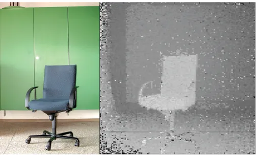
Still in the group of the range sensors, there is the Mesa Imaging SR4000 (18). This sensor, presented in Figure 7, is similar to a camera but instead of acquiring an optical image, it measures distances. It can be perceived as each of its pixels being an infra-red sensor, each taking a measure of the distance between themselves and the nearest non-transparent object. The result will be a map of distances from each pixel of the sensor to the object being measured like the one presented in Figure 8, where smaller distances correspond to lighter colours.

(21)

Figure 8. - An office chair (left) and as viewed by a SR4000 sensor (right).

This sensor is 6.5 cm wide, 6.5 high, 6.8 long and weights 470 g. Although smaller than the SICK LMS200, this sensor gains, to some extent, over some of the great advantages of the former sensor because despite having a range of only 5m, it has more or less the same resolution (1cm in range and 0.23º in angle) and it too is still fast at returning measures (up to 54fps with a 176x144 grid sensor which corresponds to a maximum of 176x144x54=1368576 measures per second). Despite having only 43.6º in horizontal angle, it has the great advantage that it performs measurements directly in 3D without the need of a tilt unit due to its vertical angle of 34.6º (compared to 0º of the SICK LMS200).

2.2 State of the Art in Vision Sensors

2.2.1 Stereo Pair of Cameras

Another method of generating 3D maps is the usage of a stereo pair of cameras. This method is relatively complex and demands a great deal of computing power to be performed in real time with negligible delay. Figure 9 shows the view from a stereo pair of cameras.

(22)

Figure 9. - View from a stereo pair of cameras.

Performing measurements from a pair of stereo images involves sophisticated algorithms of image processing to detect and match the objects from both images, like presented in Figure 10, and to extrapolate the distances of the objects relative to the robot (11), like presented in Figure 11. The distance between the robot and an object will depend on the distance that separates both cameras and on the position the object has inside each image.

(23)

Figure 11. - Position of an object (in green) inside a stereo pair of images.

As can be noticed in Figure 10, the same object in both images has slightly different shapes due to the difference in perspective between the cameras, which is one of the difficulties encountered when trying to match objects in a stereo pair of images.

Measuring distances from a stereo pair of images as the added difficulty of having to deal with problems like the illusion of having different colours, even that an object has really only one, due to the fact that the illumination is not uniform all around every object and the cameras will capture that difference of illumination as being several colours, some darker than others. Figure 12 shows an office room that was captured with a pair of stereo cameras, was processed to build the map and finally was covered with textures to help humans visualize the environment.

Figure 12. - Office reconstructed after the real one had been captured by a stereo pair of cameras and processing had occurred.

(24)

2.2.2 Omnidirectional Camera

Currently, there are techniques of capturing the surroundings using just one camera. One of those techniques is by using an omnidirectional camera, like the one presented in Figure 13. It is basically a camera pointed at a mirror, usually hyperbolic, which increases the camera field of view and allows it to have a 360º horizontal by, almost, 180º vertical view of the surroundings, like demonstrated in Figure 14.

Figure 13. - An omnidirectional camera sensor.

Figure 14. - Illustration of the operation of an omnidirectional camera.

In Figure 14, the upper black line represents the mirror and the bottom black line represents the camera sensor. The grey solid lines represent the paths of the light and the grey dashed line represents the middle of the camera-mirror setup with their corresponding focal points, a grey dot at the bottom and a small grey circle on top of the grey dashed line

(25)

respectively.

A view from an omnidirectional camera perspective is presented in Figure 15. Notice that the black circle at the centre of the image is the camera and that the objects at the edges of the image are stretched.

Figure 15. - View of an office from an omnidirectional camera.

As can be deduced from Figure 15, to process the image, it is required the application of an algorithm that performs the inverse of the distortion of the image, which can represent a significant overhead of processing, depending on the type of mirror and on the order of the equation chosen to approximate the effects of the mirror.

Although relatively more complex to process and calibrate than the stereo pair of cameras, mainly because of the distortion of the mirror, a single omnidirectional camera can be used to measure distances to objects (20).

2.2.3 Fish-eye Camera Lens

Still in the group of vision technology, and also using just one camera, is the fish-eye lens. This type of lens, shown in Figures 16, is in reality a group of lenses, as presented in Figure 17, that are combined in a manner that increases the field of view of a camera by compressing the scene being captured to fit the normal field of view of the camera, as presented in Figure 18. The photo of Figure 18 was taken with the lens of Figure 16.

(26)

Figure 16. - Fish-eye lenses.

(27)

Figure 18. - View from a fish-eye lenses.

Much like the omnidirectional camera, images taken using this technique are also more complex to process than images taken with the stereo pair of cameras due to the distortion of the lenses which have to be counteracted by an algorithm that performs the inverse of the distortion of the lenses.

2.3 Additional Range Sensors

Returning to the range sensors, there are two basic sensors that, nowadays, are not usually used to measure distances but to detect if a collision is imminent. Those sensors, presented in Figure 19, are the sonar and the infra-red, respectively left and right. Small dimensions, lightweight and low power consumption are some of the characteristics these sensors possess.

(28)

Although they lack precision for great distances, specially in harsh conditions, it is not too affected at close range. Due to the fact that these sensors are mainly used to detect the imminence of a collision, their presence in numbers is usually higher than any other sensor placed on a robot and usually cover the robot's body around a specified height.

2.4 Summary

In this chapter, the state of the art in sensor technology used in robotic search and rescue for mapping was presented along with a brief description of each sensor. The sensors described were the SICK LMS200, the HOKUYO URG-04LX, the Mesa Imaging SR4000, the stereo pair of cameras, the omnidirectional camera and the fish-eye lens. There were also presented two sensors, the infra-red and the sonar, that are not usually used for mapping.

(29)

3 Project and Implementation

This chapter presents the biggest part of the work performed throughout the thesis. It explains the 3D mapping methodology chosen, presents its implementation and justifies all the decisions taken about the robot's hardware and software architectures.

3.1 Mapping Strategy

There are some characteristics that are desirable in a search and rescue robot. Some of these characteristics are presented in Table 5.

Table 5. - List of some desirable characteristics in a search and rescue robot.

Characteristic

number Characteristic description

1 Small dimensions to allow the robot to reach tight places.

2 Light to allow easier movement and manoeuvring, and less disturbance of the surroundings. 3 Long operational range to map the entire area and, preferably, find all victims before the battery

is depleted.

4 Produce accurate maps, both for its own navigation and the human rescue teams. 5 Detects 100% of the victims.

6 Flawless localization, meaning that it will always know exactly where it is and where it has been.

7 Flawless navigation, meaning that, if possible, it can always find a way to reach its destination that inflicts the least possible disturbance in the ambient.

8 Moves quickly but without compromising the stability of the environment, meaning that it does not hit objects in its surroundings neither it provokes collapses of objects (like debris).

The first three characteristics of the list can be achieved by using the least possible amount of reduced size low power sensors. The third characteristic will be augmented proportionally to the sensors decrease in power consumption. The partial solution for the last characteristic of the list is somewhat related with the solution for the first three because, if the sensor count is low and the sensors have small sizes, then the robot can have smaller dimensions, which will make it lighter and demand less binary from the engines, translating any spare binary in quickness of movement, which solves the quickness part of that characteristic of the list.

In order to have the fewest sensors as possible, the best way is for the sensors to have some mobility instead of being statically placed on the robot. By installing them in a moving

(30)

platform, one single sensor can replace several others and still return equivalent measurements. It is stated equivalent measures because the actual measure presented by the sensor will be different but the resulting computed measure will be equal. With an increased mobility allied to a sweeping tactic, it is possible to that single sensor to return even more measurements than all the others statically placed, making it possible to obtain a 3D map of part of the world.

By optimizing the placement of the sensor sweeping platform in the robot and carefully choosing the sensors that are installed in it, we can discard most of the other sensors that usually cover the robot's body like touch sensors, to detect impacts, or sonars, to detect proximity, which also contribute to the weight of the robot.

To produce the most accurate maps (characteristic four in the list), a sensor fusion algorithm should be used to combine all sensor measures in order to take all the individual errors of the sensors and minimize the final error.

3.2 Constraints

The proposed mapping strategy imposes some constraints on the shape of the robot's body, sensors used and their placement. Those constraints are also related to the intended characteristics of the robot. Table 6 lists the constraints and the reasons why they are required.

Table 6. - Constraints for the robot and the reasons why they are required.

Constraint Reasons

Use just one sensor of each type, if

possible. To reduce the weight of the robot and increase the lifetime of the battery. Sensors should be as small and light as

possible To further decrease the weight of the robot, the energy spent and, at the same time, improve its manoeuvrability, due to the decreased weight and size, and improve its range, due to the extended battery time.

Mount all sensors required in a moving

platform. This will allow the use of the same sensors to create a 3D map of part of the world without moving the robot's body. The moving platform should have very

small movement constraints. This will allow the mapping of a bigger part of the world without moving the robot's body and, thus, without possibly introducing errors due to the change of position of the robot.

The moving platform should be placed in one of the extremities of the robot's body, away from any other part of the robot.

Without any other part of the robot in the way of the sensors, more of the world can be captured in one sweep of the moving platform. Also, there is no need to introduce algorithms to filter the parts of the robot from the sensors measurements.

Sensors should be able to scan the ground

in front of the robot. In order to detect holes or obstacles that prevent the robot's movement, or any other hazardous that can risk the integrity of the robot.

Sensors should be able to detect obstacles

on top of the robot. To be able to measure the height of the map on that position and allow an evaluation of the stability of the structure by the engineers of the search and rescue team.

(31)

3.3 Robot Hardware Architecture

3.3.1 Desired Architecture

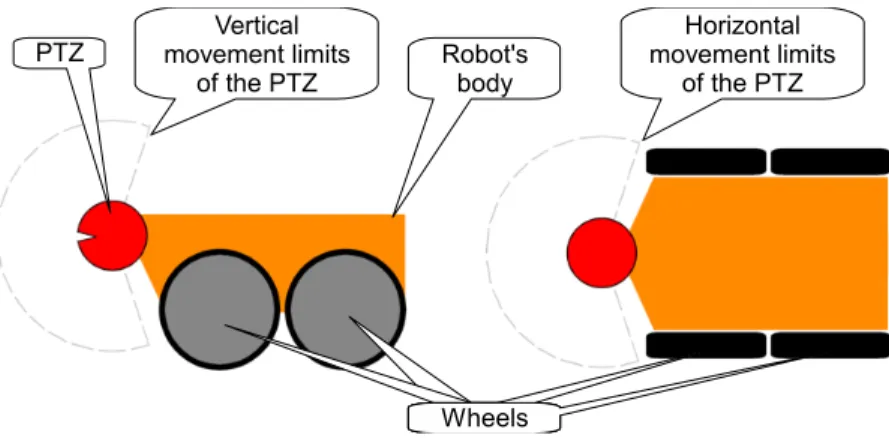
A robot architecture, that was thought to comply with the constraints, is the one in Figure 20. It is composed of a body with four wheels setup as a differential steering wheel system, one GroundTruth sensor mounted in the robot's body, one Pan-Tilt-Zoom (PTZ) platform placed in the frontal part of the robot's body, and finally one infra-red (IR) sensor and one sonar sensor, both mounted on the PTZ to perform measurements of the environment in order to generate the map. The PTZ would be able to move at least 90º in each direction (up/down/left/right) from a central position, due to its base be mounted vertically, and the sensors field of view would not be obscured by any part of the robot.

PTZ movement limits Vertical

of the PTZ Robot's body

Wheels Wheels Horizontal movement limits of the PTZ Wheels Wheels

Figure 20. - Schematic of the desired implementation of the robot.

3.3.2 Implemented Architecture for Testing

Due to lack of knowledge in 3D image editing, the desired robot architecture was not implemented. Instead a modified cut-down version of the P2AT shown in Figure 21, which already exists in USARSim, was used for testing purposes.

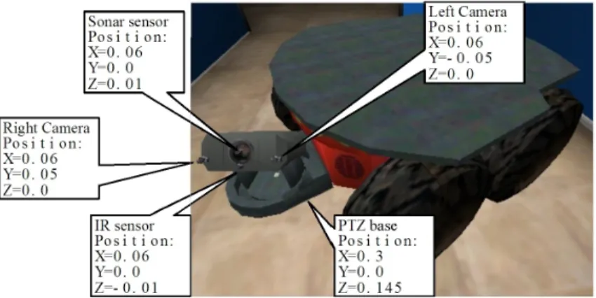
The P2AT already possessed some of the most significant characteristics we expected. It was striped of all its sensors except the ground truth, one sonar, one IR and the camera. The original P2AT has only one camera but a second one was added to allow the sensors to occupy the central position of the PTZ where the camera of the original P2AT was. The cameras were moved to the extremities of the PTZ and were left on the robot to enable us to see were the PTZ is pointing, and give an estimate to where the sensors are pointing, and did not contribute to the generation of the map. The ground truth sensor remained in the physical centre of the robot's body and the two sensors left (IR and sonar) were moved to the PTZ platform. Unfortunately, I have not been able to rotate the PTZ base into a vertical position, so it was still placed in the frontal part of the robot but in a lowered position that allowed the ground in front of the robot to stay in the sensors line of sight when the PTZ is pointing down.

(32)

The modified version of the P2AT is presented in Figure 22 along with the relative placement of its sensors and PTZ.

Figure 21. - Image of the original P2AT in USARSim, the robot modified to be used for testing.

Figure 22. - The modified P2AT robot and its sensors relative placement.

The positions of the sensors shown in Figure 22 are relative to the (x=0;y=0;z=0) point of the part of the robot they are attached to. The complete configuration of the robot, and how to perform it, is presented in a later point of this document.

3.3.3 Implementation of the Testing Robot

Since the robot used in this work is based in a pre-existing one, implementing it is very easy. USARSim installs two files in the "System" folder of UT2004 called "USARBot.ini" and "USARMisPkg.ini" that are used to provide the configuration of the robots and the configuration of the mission packages, respectively.

(33)

Starting with the mission package, the PTZ moving constraints must be altered to allow the PTZ to move as much as we desire for this work. Luckily, the physical design of the PTZ parts allows for this, otherwise, changing this settings would not have any effect since UT2004 uses the part design to simulate the rigid body. For this work the constraints were removed completely in the configuration file and are performed instead by the software robotic agent. To remove the constraints, locate the text "[USARMisPkg.CameraPan]" and "[USARMisPkg.CameraTilt]" and replace the corresponding MinRange values by 1 and the MaxRange values by 0. When MinRange is set to be greater than MaxRange, the corresponding part does no have any constraints.

Now, the robot must be created. To create the robot, it is only necessary to copy the "P2AT.uc" file in the "USARBot\Classes" folder of UT2004 and paste it with the name of our robot. The robot in this work was called "Mapper", so the pasted file's name must be changed to "Mapper.uc". Be aware that all text mentioned here is case sensitive, including the name of the file. Next, the file of the new robot ("Mapper.uc") must be opened in a simple text document, like notepad, and the text presented in Table 7 must be replaced from the original to the modified. After this step, USARSim must be compiled. To perform the compilation is just necessary to click the link "Compile" under the "Programs\USARSim" folder in the "Start menu" of the Windows®_{OS like it was presented earlier in this document. If no errors occur,}

a message of successful completion will be presented

Table 7. - Text replacement in "Mapper.uc" robot definition file.

Original Modified

class P2AT extends SkidSteeredRobot

config(USARBot); class Mapper extends SkidSteeredRobot config(USARBot); KParams=KarmaParamsRBFull'USARBot.P2AT.KPa

rams0' KParams=KarmaParamsRBFull'USARBot.Mapper.KParams0'

Finally, the robot must be configured. To configure it, the file "USARBot.ini" must be edited and the configuration of the P2AT robot must be copied. That is a part of the file like the one in Table 8. Then it must be pasted and modified to remove unnecessary sensors. In the end, it must be like the configuration in Table 9.

Table 8. - P2AT robot configuration

P2AT robot configuration [USARBot.P2AT] bDebug=False Weight=14 Payload=40 ChassisMass=1.000000 (...) Sensors=(ItemClass=class'USARBot.GroundTruth',ItemName="GroundTruth",Position=(X=0.0,Y=0.0,Z=-0.0),Direction=(Y=0.0,Z=0.0,X=0.0))

(34)

Table 9. - Mapper robot configuration

Mapper robot configuration [USARBot.Mapper] bDebug=True Weight=14 Payload=40 ChassisMass=1.000000 MotorTorque=40.0 bMountByUU=False batteryLife=50000 JointParts=(PartName="RightFWheel",PartClass=class'USARModels.P2ATTire',DrawScale3D=(X=1.0,Y=0.5 5,Z=1.0),bSteeringLocked=True,bSuspensionLocked=true,Parent="",JointClass=class'KCarWheelJoint',Parent Pos=(Y=0.20399979,X=0.13199987,Z=0.13104749),ParentAxis=(Z=1.0),ParentAxis2=(Y=1.0),SelfPos=(Z=-0.0),SelfAxis=(Z=1.0),SelfAxis2=(Y=1.0)) JointParts=(PartName="LeftFWheel",PartClass=class'USARModels.P2ATTire',DrawScale3D=(X=1.0,Y=0.55, Z=1.0),bSteeringLocked=True,bSuspensionLocked=true,Parent="",JointClass=class'KCarWheelJoint',ParentPo s=(Y=-0.20399979,X=0.13199987,Z=0.13104749),ParentAxis=(Z=1.0),ParentAxis2=(Y=1.0),SelfPos=(Z=-0.0),SelfAxis=(Z=1.0),SelfAxis2=(Y=1.0)) JointParts=(PartName="RightRWheel",PartClass=class'USARModels.P2ATTire',DrawScale3D=(X=1.0,Y=0.5 5,Z=1.0),bSteeringLocked=True,bSuspensionLocked=true,Parent="",JointClass=class'KCarWheelJoint',Parent Pos=(Y=0.20399979,X=-0.13199987,Z=0.13104749),ParentAxis=(Z=1.0),ParentAxis2=(Y=1.0),SelfPos=(Z=-0.0),SelfAxis=(Z=1.0),SelfAxis2=(Y=1.0)) JointParts=(PartName="LeftRWheel",PartClass=class'USARModels.P2ATTire',DrawScale3D=(X=1.0,Y=0.55 ,Z=1.0),bSteeringLocked=True,bSuspensionLocked=true,Parent="",JointClass=class'KCarWheelJoint',ParentP os=(Y=-0.20399979,X=-0.13199987,Z=0.13104749),ParentAxis=(Z=1.0),ParentAxis2=(Y=1.0),SelfPos=(Z=-0.0),SelfAxis=(Z=1.0),SelfAxis2=(Y=1.0)) MisPkgs=(PkgName="CameraPanTilt",Location=(Y=0.0,X=0.3,Z=0.145),PkgClass=Class'USARMisPkg.Cam eraPanTilt') Cameras=(ItemClass=class'USARBot.RobotCamera',ItemName="CameraLeft",Parent="CameraPanTilt_Link2 ",Position=(Y=-0.05,X=0.06,Z=0.0),Direction=(Y=0.0,Z=0.0,X=0.0)) Cameras=(ItemClass=class'USARBot.RobotCamera',ItemName="CameraRight",Parent="CameraPanTilt_Link 2",Position=(Y=0.05,X=0.06,Z=0.0),Direction=(Y=0.0,Z=0.0,X=0.0)) HeadLight=(ItemClass=class'USARBot.USARHeadLight',ItemName="HeadlightLeft",Parent="CameraPanTilt _Link2",Position=(Y=-0.05,X=0.08,Z=-0.03),Direction=(Y=0.0,Z=0.0,X=0.0)) HeadLight=(ItemClass=class'USARBot.USARHeadLight',ItemName="HeadlightRight",Parent="CameraPanTi lt_Link2",Position=(Y=0.05,X=0.08,Z=-0.03),Direction=(Y=0.0,Z=0.0,X=0.0)) Sensors=(ItemClass=class'USARBot.SonarSensor',ItemName="Sonar",Parent="CameraPanTilt_Link2",Positio n=(Y=0.0,X=0.06,Z=0.01),Direction=(Y=0.0,Z=0.0,X=0.0)) Sensors=(ItemClass=class'USARBot.IRSensor',ItemName="IR",Parent="CameraPanTilt_Link2",Position=(Y= 0.0,X=0.06,Z=-0.01),Direction=(Y=0.0,Z=0.0,X=0.0)) Sensors=(ItemClass=class'USARBot.GroundTruth',ItemName="GroundTruth",Position=(X=0.0,Y=0.0,Z=-0.0),Direction=(Y=0.0,Z=0.0,X=0.0))

The cameras and the headlights can be removed from the file because they are not used by the software robotic agent, but they may be handy if someone intends to watch the robot in action. Actually, if the robot had been implemented as a real robot, the cameras and headlights would not have been inserted.

From this point on, if the simulator is started and the "Mapper" robot invoked, it should appear on the scenario.

(35)

3.4 Sensors and Sensor Models

3.4.1 In USARSim

In USARSim, the IR sensor is modelled as a straight line that starts at the sensor and ends when it intersects the first non transparent object. It then returns the length of the line. The sensor has a maximum range and an error that increases linearly with the distance of the point measured. However, its characteristics can be modified in the “USARBot.ini” configuration file.

The sonar is modelled by many straight lines starting at the sensor, projecting themselves away from the sensor, inside its cone of action, and ending in the first object (transparent or not). After one pass of measurements, the length of smallest line is returned. Similarly to the IR sensor, the sonar sensor has a maximum range and an error that increases linearly with the distance of the point measured. It also has an angle that defines the sonar's cone of action.

The sensors with their properties, their descriptions and the values they were configured to in this work are listed in Table 10.

Table 10. - List of sensors, their properties, property descriptions and the values they assume for this work.

Sensor name Sensor property Property value Property description

Sonar

Maximum range 5 m The maximum range of the sensor in normal conditions Maximum error 0.05 m The maximum error of the sensor in normal conditions. The _{error is a function of distance.} Angle of cone 0.0873 rad It is the line of sight angle of the sensor. Any object outside _{this angle is not sensed.} Position (X=0.06,Y=0.0_{,Z=0.01) m} The relative position of the sensor in regard to the centre of _{tilt unit of the PTZ.}

IR

Maximum range 5 m The maximum range of the sensor in normal conditions Maximum error 0.05 m The maximum error of the sensor in normal conditions. The _{error is a function of distance.} Position (X=0.06,Y=0.0 _{,Z=-0.01) m} The relative position of the sensor in regard to the centre of _{tilt unit of the PTZ.}

In the experiments conducted, which are detailed in a later point of this document, for the particular case of the measurements without error that serve to get the comparison references, the error was set to zero.

(36)

3.4.2. In Robotic Software Agent

Each measurement from the IR or the sonar sensors will be converted into a line or cone of points, respectively, were each one of those points will have a probability associated with it. That probability will reflect the probability of that point being occupied and it depends on the sensor's model of uncertainty. Keep in mind that a line can be understood as a special case of a cone where the angle of the cone is zero. This approach allows the same model of uncertainty to be used with both types of sensors.

The model of uncertainty used in this work will be the one represented in Figure 23 (10) and it divides the sensor's action range in three regions. Region I is the region where the points are probably occupied. Region II is the region where the points are probably empty. Region III is the region where it is unknown if the points are occupied or empty.

Figure 23. - Representation in 2D (left) and 3D (right) of the sensor model of uncertainty removed from (10).

The regions' limits are determined by using the maximum range of the sensor and the maximum error for the measured distance. If a sensor measures the distance A and the sensor model states that, for that distance, the maximum error is E, then the limit that separates Region I from Region II is at a distance of A-E from the sensor, and the limit that separates Region I from Region III is A+E. In this work, the sensor model for the error over the distance presented in Figure 24 is used for both sensors. The curve presented is also the default for range sensors in USARSim but can easily be modified.

(37)

Figure 24. - Example of a sensor model for the error.

The probability of each point will be calculated using one of the two methods mentioned earlier in this document. The first is the dumb method that updates the probabilities using a mean and the other is the Bayesian method.

For the dumb method, the sensor model presented will be applied to each measure from the sensor but the error will always be regarded as zero, meaning that Region I will be constituted solely by the points that present themselves at the measured distance and will be given the probability of 100% occupied. All other points between the sensor and the measured distance will be given the probability of 0% occupied. If any of those points already exists in memory, their probabilities will be updated by performing the mean value of the currently given probability with their old value of probability of occupancy.

For the Bayesian method, the formulas used for the calculation of the probabilities are (1) to (3) and belong to regions I to III of Figure 23, respectively.

P occupied = R−r R  β−α β 2 ×maxoccupied (1)

(1) - Equation for the probability of Region I in the Bayesian method

P occupied =1− R−r R  β−α β 2 (2)

(2) - Equation for the probability of Region II in the Bayesian method

P occupied =unknown ; do nothing ₍₃₎

(3) - Equation for the probability of Region III in the Bayesian method

Where R is the sensor's maximum range, r is the measured distance from the sensor to the point being calculated, β is the beam half angle, α is the angle between the line that connects the centre of the sensor to the point being calculated with the line that defines the centre of the

(38)

cone, and maxoccupied is a pre-defined value that defines the assumption that a point is already

occupied before any measurements are made. In the special case of the IR sensor, since there is no β nor α, the term β −α_β in the above formulas is zero.

After calculating the probability of a measured point using formulas (1) to (3), the probability of each point in the world is updated using formula (4)

P_worldoccupied = P×P−1

P× P−11.0−P×1.0− P−1 (4)

(4) - Equation for the probability update in the Bayesian method

Where P is the probability of the measured point and P-1 is the previous probability of that

point in the world. If there is no previous point (P-1) then maxoccupied is used instead.

3.5 Robot Software Architecture

3.5.1 Hardware Emulation

The robot's computational platform was built with two main purposes in mind. One was to allow to count the number of instructions used to implement the proposed algorithms and, the other, was to allow a quick conversion of the algorithms from the emulated platform to a real robot. With this in mind, the robotic agent architecture was developed to emulate the hardware of a real robot. It emulates a 32bit single threaded computer with separate instruction and data pointers, memories and buses, where all peripherals are regarded as memory positions. There is no floating point arithmetic, meaning that all operations are performed over integers including functions like sine, cosine, tangent, etc. Also, to keep the architecture as simple as possible, there are no advanced features like stack, internal registries (except for the instruction and data pointers), cache or memory management hardware and all memory positions correspond to a 32bit integer variable.

Figure 25 shows the emulated hardware architecture of the entire robot. The white blocks are the "real" hardware of the robot and the grey blocks are the classes that emulate the hardware. We can see that the "real" hardware is composed of a CPU, RAM and peripherals. The peripherals are sub-divided in input and output peripherals. Input peripherals contain Sonar, IR, robot position and posture, light intensity information and light toggle information. Output peripherals contain light intensity, light toggle, wheels speed, pan and tilt position.

(39)

Figure 25. - Emulated hardware architecture.

The blocks that emulate the hardware do not translate to hardware in a real robot. Those blocks handle the communications with the simulator, emulate the RAM, emulate the sensors and actuators, and implement the abstraction layer that hides the actual implementation of the sensors, actuators and RAM, and treats them as memory positions.

For the emulation to be complete, a set of assembly like instructions was created for the emulated CPU. These instructions were loosely based on the 80C51 microprocessor instructions but were implemented in such a way that the programmer could benefit to some extent, in the assembly, from characteristics typical of high level languages like encapsulation. The different types of instructions and their purpose is presented in Table 11. Since the complete set of instructions is too extensive, it is presented only in Annex B along with the corresponding syntax, usage description and examples. The parameters received by an instruction are each separated by one space. It is assumed that all instructions take only one clock cycle to execute.

(40)

Table 11. - Different types of instructions of the emulated CPU. Instruction type Instruction type name Description A Conditional function call

In this instruction type a function is called if, or while, the value of a certain variable is true or when the comparison of the values of two certain variables is true. Most of the instructions of the emulated CPU belong to this type of instructions.

B Arithmetic This instruction type includes all the arithmetic operations over the value of one or two variables (attribution, sum, subtraction, multiplication and division) as well as all calculations performed over the value of a single variable like sine, cosine, tangent, etc.

C Memory

addressing With only two instructions, this instruction type allows for indirect memory manipulation. A variable can have the address of another variable saved as its value and the value of a variable can be loaded into the memory pointer as an address.

As one can conclude from Table 11 and Annex B the set of instructions is very limited but, as will be demonstrated, contains all the necessary instructions to process all the algorithms required by this work.

Carefully analysing the instructions in Annex B, one can conclude that most instructions are somewhat easy to understand and use, and that the usage of the memory addressing instructions can be a little confusing. To try and clarify the usage of each instruction type, a detailed description of each follows.

The instruction type easiest to understand is the arithmetic. These are ordinary calculations over variables and are straightforward to use. Figure 26 shows an example of the calculation of the sine of the sum of two numbers. The variables used are named a, b, c and d where a and b are the numbers to be added, c will hold the result of the sum and d will hold the result of the sine.

...

add a b c sin c d ...

Figure 26. - Example of two arithmetic instruction type.

The conditional function call type of instructions are used to perform comparisons and call functions. All comparisons were defined to call a function to impose the modularization of the code, making it easier to analyse and implement. Figure 27 shows an example of a conditional function call type of instructions where two numbers are compared and the smaller number is subtracted to the greater number. The variables used are named a,b and c where a and b are the numbers to be compared and c will hold the result of the subtraction. The function called when a is greater than or equal to b is named add1 and the function called when a is smaller than b is named add2.

(41)

...

ifge2 a b add1 add2 ... add1: sub a b c ret ... add2: sub b a c ret ...

Figure 27. - Usage example of an if instruction of the conditional instruction type.

When a function returns, it will return to the line of code following the function call except if the function was called with an while instruction. In the later case, the function will return to the same line of code it was called from and will execute the next line of code after the while instruction only when the comparison becomes false. In the case of the example in Figure 27 either function add1 or add2 will return to the instruction following the if (ifge2) instruction. Figure 28 shows the example of the usage of the while instruction by recursively calculating the factorial of a number. The variables are named r, t and n where r will hold the result of the calculation, t is a temporary variable and n is the wanted number of the factorial.

... mov r 1 mov t n wg t 1 factorial ... factorial: mul r t r sub t 1 t ret ...

Figure 28. - Usage example of a while instruction of the conditional instruction type.

(42)

implemented to allow the usage of pointers, arrays, linked lists, etc. The easiest way to demonstrate its usage might be with an example. Figure 29 shows an example usage of the memory addressing instruction type by calculating the sum of the values of an array addressed by a variable. Like in many languages an array is implemented as consecutive memory positions were position zero is also the base address of the array. So, to access position x of an array, one needs to sum x to the base address of the array. The variables are named v0, v1, ..., vn, a, n, t1, t2, s and i where v0 to vn are the array positions stored in sequential memory positions, a will hold the base address of the array, n is the number of elements of the array, t1 is a temporary variable that will hold the address of the current position of the array, t2 is a temporary variable that will hold the value of the memory position addressed by t1, s will hold the sum of the elements of the array and i is a counter that is used to address an element of the array. ... ma v0 a mov i 0 mov s 0 wl i n sum1 ... sum1: add a i t1 mv t1 t2 add s t2 s add i 1 i ret ...

Figure 29. - Usage example of the memory addressing instruction type.

3.5.2 Software Emulation

To improve the speed of the program that emulates the robot hardware architecture and software architecture, the actual instruction set for the CPU was not implemented but translated into equivalents in the language used to program. That language was C++ and Table 12 presents some example translations. Annex C presents the full list of equivalences between instructions as well as detailed descriptions of each instruction.

(43)

Table 12. - Some examples of conversions between the emulated CPU instructions and C++.

CPU Instruction CPU Syntax/Example C++ Syntax/Examples (in italic)

call function call f0 f0();

if greater than or equal call function ifge v0 v1 f0 if(v0>=v1) f0();

if less than or equal return iflr v0 v1 if(v0<=v1) return;

while greater than call function wg v0 v1 f0 while(v0>v1) f0();

move value to variable mov v0 v1 v1=v0;

divide values and store result div v0 v1 v2 v2=v0/v1;

and v2 can be v0, v1 or another variable divide values and store remainder rem v0 v1 v2 v2=v0%v1;

or

v2=v0-(v0/v1)*v1;

and v2 can be v0, v1 or another variable store sine of value sin v0 v1 v1=sin(v0);

and v1 can be v0 or another variable get memory address value mv v0 v1 v1=*v0;

Looking closely at the list of all instruction equivalences in Annex C, one realizes that most conversions are easy to understand and straightforward to implement. But the instructions related to memory addressing can be a little difficult to realize their true potential. Figure 31 and Figure 32 show, in C++ and emulated CPU assembly respectively, an example of translation for an application using the memory addressing instructions. In that example, it is performed the sum of the elements of a linked list implemented in two arrays, one of values and other of indexes to the next element of the list. Assume that, if the next list position does not exist, the index will have a negative value. Also assume that the arrays are similar to those shown in Figure 31.

The variables are named first, list0, list1, ..., listn, index0, index1, ..., indexn, a, s and t where first is the position of the first element of the list, list0 to listn are the array positions of the list values stored in sequential memory positions, index0 to indexn are the array positions of the next elements of the list stored in sequential memory position, a will hold the value of the current element of the list, s will hold the result of the sum and t is a temporary variable to store addresses.

list[]={10,3,67,9}; index[]={2,3,-1,0}; first=1;

Figure 30. - Example of a linked list implemented using two arrays in a C like language.

(44)

... s=0; i=first; while(i>=0){ a=list[i]; s+=a; i=index[i]; } ...

Figure 31. - Example in C++ of the sum of the elements of a linked list implemented using two arrays.

... mov s 0 ma list0 list ma index0 index mov i first wge i 0 sum1 ...

sum1: add list i t mv t a add s a s add index i t mv t i ret ...

Figure 32. - Example in emulated CPU assembly instructions of the sum of the elements of a linked list implemented using two arrays.

In reality, to minimize the risk of errors occurring while running or compiling the program, the functions in C++ do receive parameters by reference instead of being passed through

(45)

global variables but this fact does not affect the translation from C++ to emulated CPU assembly as long as the names of the variables and functions are kept consistent.

3.6 Software Robotic Agent

With the hardware and software emulations defined, the software robotic agent can be programmed to order the robot in the simulator to execute actions, perform measurements and build the 3D map of the scenario. The robotic software agent is composed of several threads of execution, each with its functionality, and many functions that perform specific tasks like building the sensor cone for the model of uncertainty. One thread executes the hardware abstraction layer, other the parsing of the messages from the simulator and other executes the main program.

3.6.1 Main Program

The main program thread is responsible for managing and coordinating all other threads, and for imposing an order of execution of the tasks to be performed by the software robotic agent. The block diagram of the main program thread execution flow is provided in Figure 33. The grey block is the starting point. A more detailed list of the tasks of the main program thread and their corresponding execution flow is listed in Table 13 for better comprehension.

(46)