Tít
ulo
N
om
e d
o A
uto
r
This work aims to optimize a 6- RUS parallel robot
to determine the optimal active joints locations
(position and orientation) for a flight simulation
task using a PSO (Particle Swarm Optimization)
algorithm to escape from local minima and an
Interior Point algorithm to accelerate the search for
the optimum in the region indicated by PSO i.e.
Interior Point algorithm work to find bottom of the
valley indicated by PSO.
Advisor: Aníbal Alexandre Campos Bonilla
Joinville, 2015
MASTER DISSERTATION
ORIENTATION WORKSPACE
OPTIMIZATION FOR A 6-RUS
PARALLEL ROBOT
ANO
2015
CLO
DO
ALD
O S
CH
UT
EL
FU
RT
AD
O N
ET
O |O
RIE
NT
AT
IO
N W
OR
KP
AC
E
OP
TIM
IZA
TIO
N F
OR
A
6-R
US
PA
RA
LLE
L R
OB
OT
SANTA CATARINA STATE UNIVERSITY – UDESC
TECHNOLOGICAL SCIENCES CENTER – CCT
POST GRADUATION PROGRAM IN MECHANICAL ENGINEERING– PPGEM
CLODOALDO SCHUTEL FURTADO NETO
Orientation Workspace Optimization For a 6-RUS
Parallel Robot
Dissertation submitted to Santa
Catarina State University as part of the requirements for obtaining the degree of Master in Mechanical Engineering.
ADVISOR: Dr. Aníbal Alexandre Campos Bonilla
Joinville, SC
F992o Furtado Neto, Clodoaldo Schutel
Orientation workspace optimization for a 6-RUS parallel robot / Clodoaldo Schutel Furtado Neto. – 2015.
256 p. : il. ; 21 cm
Advisor: Aníbal Alexandre Campos Bonilla
Bibliography: p. 123- 127
Dissertation (master) –Santa Catarina State University, Technological Sciences Center, Post Graduation Program in Mechanical Engineering,
Joinville, 2015.
1. Parallel Robot 2. Flight Simulator3. 6-RUS 4. Singularity 5. Optimization I. Bonilla, Aníbal Alexandre Campos . II. Santa Catarina State University, Post Graduation Program in Mechanical Engineering. III. Title.
I would like to thank the Mechanical Engineering Department of
UDESC for accepting me to carry out this master. In a special way express my
gratitude.
To Dr. Aníbal Alexandre Campos Bonilla, for guiding me with
enthu-siasm in this work. I have great affection and appreciation for you, admire as a
person and also for your professionalism.
My colleagues and friends Guilherme Espindola, Guilherme Faveri
and Rodrigo Trentini, who help me in some stages of this work.
To my mother who taught me my values, had the enormous task of
educate my brother and I alone and always sought the best for us.
My brother who was always by my side and made everything in my
life more easier.
My dear friend Ana Maria Franco who encouraged me to enter this
master, helped me when I faced obstacles and especially for your friendship
and affection.
To my dear friend Thiago Kavilhuka who is gone and left many
longing.In memoriamThiago Kavilhuka.
To God who gave me health and strength of will to not discourage
FURTADO, C.Orientation Workspace Optimization For a 6-RUS
Paral-lel Robot.2015. 256 p. Dissertation (Master in Mechanical Engineering – Area: Design, Analysis and Optimization of Mechanical Systems) – Santa
Catarina State University, Post Graduation Program in Mechanical
Engineer-ing, Joinville (Brazil), 2015.
The Santa Catarina State University built a flight simulator based on 6-DoF
axisymmetric parallel robot which incorporates virtual reality immersion
environment. This flight simulator presents 6-RUS kinematic chain which is
the second most common architecture for this application. Hunt proposed this
chain architecture early in 1983. Parallel robots are closed-loop mechanisms
that present good performance in terms of accuracy, rigidity and ability to
manipulate large loads. This work aims to optimize a 6- RUS parallel robot to
determine the optimal active joints locations (position and orientation) for a
flight simulation task using a PSO (Particle Swarm Optimization) algorithm
to escape from local minima and an Interior Point algorithm to accelerate
the search for the optimum in the region indicated by PSO i.e. Interior Point
algorithm work to find bottom of the valley indicated by PSO.
FURTADO, C.Otimização da Orientação no Espaço de Trabalho de um
Robo Paralelo 6-RUS.2015. 256 f. Dissertação (Mestrado em Engenharia Mecânica – Área: Projeto, Análise e Otimização de Sistemas Mecânicos) –
Universidade do Estado de Santa Catarina, Programa de Pós-Graduação em
Engenharia Mecânica, Joinville, 2015.
A Universidade do Estado de Santa Catarina construiu um simulador de vôo
de baseado robô paralelo axissimétrico com 6 DoF (graus de liberdade) que
incorpora ambiente de realidade virtual de imersão. Este simulador de vôo
apresenta cadeia cinemática 6-RUS que é a segunda arquitetura mais comum
para esta aplicação. Robôs paralelos são mecanismos de cadeia fechada que
apresentam bom desempenho em termos de precisão, rigidez e capacidade
para manipular grandes cargas. Este trabalho tem como objetivo otimizar um
robô paralelo 6- RUS para determinar os melhores localizações das juntas
ativas ( posição e orientação ) para uma tarefa de simulação de vôo usando
um algoritmo PSO (Particle Swarm Optimization) para escapar de mínimos
locais e um algoritmo de Ponto Interior para acelerar a procurar pelo ótimo na
região indicada por PSO ou seja o algoritmo de Ponto Interior trabalha para
encontrar fundo do vale indicado pelo PSO.
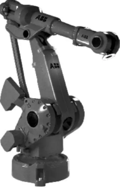
Figure 1 – ABB IRB 4400 serial robot. . . 30
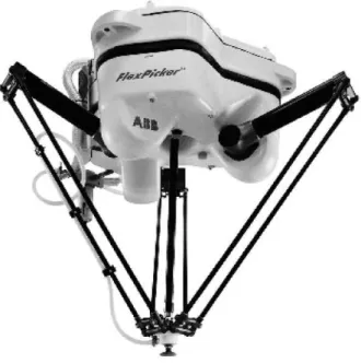
Figure 2 – ABB IRB 340 FlexPicker parallel robot. . . 31
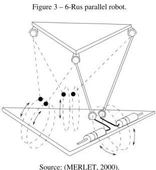
Figure 3 – 6-Rus parallel robot. . . 34
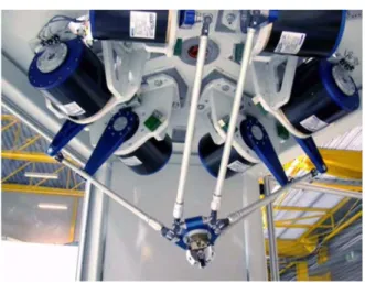
Figure 4 – IWF-robot. . . 35
Figure 5 – CEART-robot. . . 36
Figure 6 – Screw movement or twist. . . 37
Figure 7 – Twist components for a general screw kinematic pair. . . 38
Figure 8 – Wrench components. . . 43
Figure 9 – Parallel robot geometrical parameters. . . 45
Figure 10 – Vectorial chain toi-limb. . . 48
Figure 11 – Planeωifrontal view and required angles. . . 49
Figure 12 – Planeωifrontal view, geometrical details. . . 49
Figure 13 – Planeωifrontal view. . . 52
Figure 14 – Position of pointsB, andC. . . 58
Figure 15 – (a) The wrenches acting upon the end-effector. (b) and (c) Two direct singularities. . . 63
Figure 16 – Grassmann varieties of dimension 1,2,3,4,5,6. . . 66
Figure 17 – Distance between two segments. . . 79
Figure 18 – a) Grassmann variety V5a on the Hexa; b) Power based index; c) Grassman variety V5b; d) Grassman V5b based index. . . 82
Figure 19 – Flowchart for particle swarm optimization algorithm. . . 88
Figure 20 – Internal Point Algorithm. . . 91
β3,β4,β5andβ6. . . 99
Figure 23 – Active joint local system. . . 100
Figure 24 – Active Joint Angular Positionθ. . . 100
Figure 25 – Platform angular layout, where the design parameters are χj1,χj2,rpende. . . 101
Figure 26 – IWF-robot active joint location. . . 102
Figure 27 – Pitch-Roll-Yaw of an Air Plane . . . 104
Figure 28 – Axis Orientation Rotation withαfrom0oto360o . . . . 105
Figure 29 – IWF-robot Polar Graphic. . . 106
Figure 30 – CEART-robot Polar Graphic. . . 107
Figure 31 – IWF-robot direct singularity index, see red arrow. . . 107
Figure 32 – IWF-robot inverse singularity constraint. . . 108
Figure 33 – CEART-robot direct singularity index. . . 109
Figure 34 – CEART-robot inverse singularity constraint, see red arrow. 109 Figure 35 – Flowchart of MATLAB program optimization program. . 110
Figure 36 – Optimized 6-RUS Polar Graphic. . . 113
Figure 37 – Direct singularity index forY rotation, see red arrow. . . 114
Figure 38 – Passive links minimum distance. . . 115
Figure 39 – Cranks minimum distance, see red arrow. . . 115
Figure 40 – Inverse singularity constraint forY rotation, see red arrow. 116 Figure 41 – Crank 1 movement forY rotation, see red arrow. . . 116
Figure 42 – Crank 6 movement forY rotation, see red arrow. . . 117
Figure 43 – IWF-robot layout in ADAMS. . . 118
Figure 46 – CEART-robot layout in ADAMS. . . 119
Figure 47 – CEART-robot rotation inY axis, inverse singularity near
25◦. . . 120
Figure 48 – Optimized 6-RUS layout in ADAMS. . . 121
Figure 49 – Optimized 6-RUS robot torque application near direct
sin-gularity. . . 121
Table 1 – 6-RUS Robot geometrical parameters. . . 44
Table 2 – PSO coefficients values. . . 89
Table 3 – IWF-robot angles parameters. . . 101
Table 4 – IWF-robot Geometrical Parameters. . . 102
Table 5 – CEART-robot angles parameters. . . 103
Table 6 – CEART-robot Geometrical Parameters. . . 103
HDBjoint Half of Distance Between a Pair of Joints
HDBact Half of Distance Between a pair of ACTuator
APact Angles for position a Pair of ACTuator
APjoint Angles for position a Pair of JOINTs
Aact Angles for ACTuator’s orientation
MDBL Minimal Distance Between any pair of Limbs
rb Radius of the Base
rp Radius of the End-Effector
ri Length of the Crank
Ri Length of the Passive Link
e Half of Distance Between a Pair of Joints
d Half of Distance Between a Pair of Actuators
χa Angles for Position of Actuators
χj Angles for Position of a Pair of Joints
β Angles for Actuator’s Orientation
1 INTRODUCTION . . . . 29
2 PARALLEL ROBOTS . . . . 33
2.1 Robot Architectures . . . 34
2.2 Screw Theory Representation . . . 36
2.2.1 Wrench: action screw . . . 40 2.2.2 Reciprocity and rate of work . . . 42
2.3 Inverse Kinematic Problem. . . 44
3 ROBOT SINGULARITIES . . . . 57
3.1 Direct Singularity. . . 62
3.1.1 Singularity detection method . . . 63 3.1.2 Grassmann Geometry. . . 64
3.2 Singularity Closeness Measures . . . 67
3.2.1 Linear Algebra Based Measures . . . 68 3.2.2 Screw Theory Based Measures . . . 69
4 SINGULARITY POWER INSPIRED MEASURE . . . 71
4.1 Minimization Problem . . . 71
4.1.1 Twist Normalization: Invariant Norm . . . 73 4.1.2 Objective function: power inspired measure . . . 74 4.1.3 Constraints . . . 78
4.1.3.1 Inverse Singularity . . . 78
4.1.3.2 Cranks and limbs Collision . . . 79
5.1 Particle Swarm Optimization . . . 85
5.1.1 Particle Swarm Optimization with constriction factor 86 5.1.2 Configuration for Particle Swarm Optimization . . . . 88
5.2 FMINCON . . . 89
5.2.1 Interior Point Algorithm . . . 90 5.2.2 Sensitivity Analysis . . . 92
5.3 Hybrid Optimization . . . 94
6 ORIENTATION WORKSPACE OPTIMIZATION FOR
A 6-RUS PARALLEL ROBOT . . . . 97
6.1 Kinematical Performance Index for Two 6 - RUS
Parallel Robots . . . 97
6.2 Geometrical Parameters of the IWF-robot and
CEART-robot . . . 101
6.3 IWF-robot and CEART-robot Performance for Flight
simulator Task . . . 103
6.3.1 Proposed task . . . 103 6.3.2 IWF-robot and CEART-robot PERFORMANCE . . . 105
6.4 6-RUS Robot Optimization for Flight Simulator Task108
6.5 Optimization Result and Kinematic Analysis . . . 112
6.5.1 Software Tool: Matlab . . . 112 6.5.2 Software Tool: ADAMS . . . 116
6.5.2.1 CAE Analyze: IWF-robot . . . 117
6.5.2.2 CAE Analyze: CEART-robot. . . 119
REFERENCE . . . 125
8 APPENDIX A: MATLAB ALGORITHM . . . 131 8.1 Main Program . . . 131
8.2 Program 1 . . . 135
8.3 Kinematic and Screw Based Program . . . 136
8.4 Program 2 . . . 154
8.5 Function Objective Gradient . . . 155
8.6 Constraints Program . . . 159
8.7 Constraints Finite Differences Program . . . 162
8.8 Constraints Gradient Program. . . 167
9 APPENDIX B: ADAMS SCRIPT . . . 169 9.1 ADAMS Parametric Model Script . . . 169
1 INTRODUCTION
This work aims to determine the optimal value for some geometrical
parameters like active joints locations (position and orientation) for a 6-RUS
parallel robot in order to maximize the orientation workspace i.e. end-effector,
orientation.
Comparing parallel and serial robot configurations, it is observed that
parallel robots are advantageous in terms of accuracy, stiffness and ability to
manipulate large loads. Therefore, parallel robots are more suitable for tasks
that require such properties. However the small workspace, compared to serial
robots, is a drawback that researchers try to minimize, optimizing the parallel
robot parameters (MERLET, 2012).
In machining applications, a parallel robot requires the capability
to withstand large tool forces, which means that the robot structure must
transmit forces with high accuracy and high stiffness. Different applications
demand new requirement combinations which may be carry on optimizing
the robot structure, for a given task. To keep a low cost level, it is infeasible
to design customized robots for each application, therefore modularization
is needed. Modularization and optimization strategies for robots based on
parallel kinematics differ from the corresponding strategies used for robots
based on serial kinematics. Therefore, optimization and modularization of
parallel robots are interesting research tasks (BROGARDH, 2002).
As the performance of parallel robots is sensitive to their dimensions
and geometry, a given design may be optimized varying these parameters.
in-Figure 1 – ABB IRB 4400 serial robot.
Source: (SICILIANO et al., 2010)
dices in the design of a parallel robot, (MERLET, 2012; KELAIAIA; ZAATRI
et al., 2012; MERLET, 2006).
Stiffness optimization for a spatial 5-DOF parallel robot was
de-veloped using a genetic algorithm to escape from local minima (ZHANG,
2010). Barbosa, Pires and Lopes optimize the kinematic design a 6-dof
par-allel robot for maximum dexterity using a Genetic algorithm (BARBOSA;
PIRES; LOPES, 2005). Stan, Maties and Balan applied a Genetic algorithm
to multiple criteria optimization problems for 2-DOF micro parallel robot
(STAN; MATIES; BALAN, 2007).
Figure 2 – ABB IRB 340 FlexPicker parallel robot.
Source: (SICILIANO et al., 2010)
at UDESC - Ceart (Centro de Artes) in Florianópolis, from now on named
CEART-robot. This robot presents the second most common architecture for
parallel robots used in flight simulators: the 6 - RUS. This work intends to
establish a method for optimizing some robot geometrical parameters aiming
at maximizing the orientation workspace i.e. the maximum plane orientation
or twist in the fight simulator case. Aiming at optimizing this system a
work-based index is used. This index measures the robot closeness to singularities,
i.e. robot configurations where its degrees of freedom are modified. It is
evaluated for different flight simulation configuration i.e. active joint location
(FURTADO; CAMPOS; REIS, 2014).
Proposed workspace (objective function) optimization is based on
a kinematical index which is function of active joint location (optimization
parameters). The methods used for this optimization are a Particle Swarm
Optimization (PSO) algorithm and Interior Point algorithm, which is called
by MATLAB optimization function FMINCON. Initially , the PSO algorithm
optimizes, based on its metaheuristic behaviour, the problem to escape from
local minima and provides a set of optimized parameters. The Interior Point
algorithm, receives these optimized parameters and is employed to accelerate
the search for bottom of the valley indicated by the PSO as the best particles
locations.
Therefore this work provides a method for maximizing the workspace
of 6 - RUS parallel robot by optimizing the robot active joints location,
evaluat-ing the sevaluat-ingularity proximity and employevaluat-ing a hybrid approach , i.e. combinevaluat-ing
metaheuristic (PSO) and a derivative based algorithm (Interior Point).
The first step to develop this work is to determine the inverse
kinemat-ics equations, i.e. the relation between end-effector location and active joint
rotation. Differential kinematics, i.e. the relation between end-effector velocity
and active joint speed, and a singularity closeness index, used as constraint, are
determined applying the screw theory. Using MATLAB, this work develops
algorithms to perform the optimization and analyse the data. Optimized CAE
(Computed Aided Engineering) model (using MSC-ADAMS) is developed to
analyse the robot performance an evaluate the results. MATLAB and ADAMS
2 PARALLEL ROBOTS
Parallel robots, also named parallel manipulators, typically consist of
a platform connected to a fixed base by several limbs (MERLET, 2001) (see
Figures 3, 4 and 5).
An-DOF (n-degree-of-freedom) fully-parallel mechanism is
com-posed ofnindependent limbs connecting the end-effector to the fixed base.
Each of these limbs is a serial kinematic chain that hosts one or more active
joints which actuates, directly or indirectly, the end-effector (BONEV, 2003).
Due to distribution of external load, parallel robots present good performances
in terms of accuracy, rigidity and ability to manipulate large loads (MERLET,
2001).
The 6-DOF parallel robot most studied architecture is the 6-UPS.
This architecture is known as Stewart-Gough platform (FICHTER, 1986).
The Stewart-Gough platform presents a stiff architecture be cause the load
distribution is only axial and allows the use of powerful hydraulic actuators.
Motion simulators, generally, manipulate excessive loads of up to tens of tons
(BONEV, 2003).
The second most common architecture is the 6-RUS kinematic chain,
this chain architecture was proposed by Hunt early in 1983 (MERLET, 2001).
In this architecture the actuated joint is rotational, which leads to the
inter-change possibility of universal and spherical joint without any inter-change in
mechanism characteristics (BONEV, 2003). This work focus in a method to
optimize the workspace the robot 6-RUS using an index of singularity
2.1
Robot Architectures
As early as 1983 Hunt suggested a robotic architecture using this
type of chain (HUNT, 1983) (see Figure 3). This parallel robot is composed
of two platforms, one of them fixed to the ground,(base). On the base there are
six rotating actuatorsRlocated on the edges of the triangle. These actuators
are the input elements on which the active joints are located. Each actuator is
linked to the end-effector through a rod. In each rod, one tip is linked to the
crank of an actuator through an universal jointU and the other tip is connected
to the end-effector by means of a spherical jointS, as depicted in Figure 3. A
couple of rods converge on each spherical joint of the end-effector (ZABALZA
et al., 2003).
Figure 3 – 6-Rus parallel robot.
Source: (MERLET, 2000).
six degree of freedom DOF manipulator composed of six equally designed
kinematic chains, which connect a base-platform to the end-effector platform.
Each chain can be described as a serial RUS chain, whereRstands for revolute
joint,Ufor universal or cardan joint andSfor spherical joint respectively (see
Figure 21).
The revolute joints of the HEXA’s structure are the active joints,
which means that they are driven by an actuator while spherical joints in the
structure remain passive. A prototype of the HEXA parallel robot has been
designed and built at the Institute of Machine Tools and Production Technology
(IWF) in Braunschweig, Germany, from now on named IWF-robot (see Figure
4), (LAST et al., 2005).
Figure 4 – IWF-robot.
Source: (LAST et al., 2005).
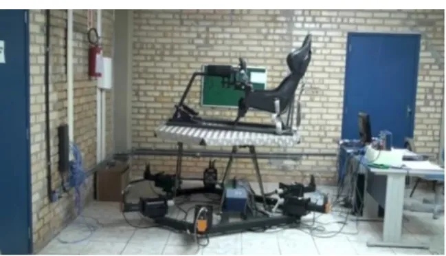
The flight simulator built at UDESC - Ceart (Centro de Artes) in
Both configurations belong to the same family, so they have the same kinematic
structure (FURTADO; CAMPOS; REIS, 2014).
Figure 5 – CEART-robot.
Source: Own Author.
2.2
Screw Theory Representation
The Mozzi theorem, states that the velocities of the points of a rigid
body with respect to an inertial reference frameO(X, Y, Z)may be
repre-sented by a differential rotation~ωabout a certain fixed axis and a simultaneous
differential translation~τ along the same axis. The complete movement of the
rigid body, combining rotation and translation, is called screw movement or
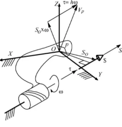
twist$. Figure 6 shows the body "twisting" around an axis instantaneously
fixed with respect of the inertial reference frame. This axis is called the screw
axis and the rate of the translational velocity and the angular velocity is called
the pitch of the screwh=k~τk/k~ωk.
The twist represents the differential movement of the body with
respect to the inertial frame and may be expressed by a pair of vectors,i.e.
Figure 6 – Screw movement or twist.
Source: (CAMPOS et al., 2011).
the body with respect to the inertial frame. The vectorV~p= [P∗
Q∗
R∗]T
represents the linear velocity of a pointP attached to the body which is
instantaneously coincident with originOof the reference frame. If there are
no points of the body coinciding with the frame originO, as in Figure 6,
a ficticious extension may be added to the body such that a point in this
extension, named pointP, coincides with the originO(see Figure 7). The
vectorV~pconsists of two components: a) a velocity component parallel to the
screw axis represented by~τ =h ~ω; and b) a velocity component normal to
the screw axis represented byS~o×~ω, whereS~ois the position vector of any
point at the screw axis.
A twist may be decomposed into its amplitude and its corresponding
normalized screw. The twist amplitudeΨis either the magnitude of the angular
velocity of the body,kω~k, if the kinematic pair is rotative or helical, or the
Figure 7 – Twist components for a general screw kinematic pair.
Source: (CAMPOS et al., 2011).
Consider a twist given by$ = [~ω ~Vp]T = [L M N P∗ Q∗ R∗]T then
the correspondent normalized screw isˆ$ = [L M N P∗ Q∗ R∗]T . This
normalized screw is a twist in which the magnitudeΨis factored out, i.e.
$ = ˆ$ Ψ (2.1)
The normalized screw coordinates (HUNT, 2003) may be defined as
of length~L, given by, ˆ $ = L M N P∗ Q∗ R∗ = ~ S ~
So×S~+h~S
(2.2)
whereS~ is the normalized vector parallel to the screw axis. Notice that the
vector(So~×S)determines the moment of the screw axis around the origin of
the reference frame.
The movement between two adjacent links, belonging to an-link
kinematic chain, may be also represented by a twist. In this case, the twist
represents the movement of linkiwith respect to link(i−1).
In robotics, generally. the differential kinematics between at pair of
bodies is determined by either a rotative or a prismatic kinematic pair. For a
rotative pair the pitch of the twist is null(h= 0). In this case the normalized
screw or a rotative pair is expressed by
ˆ $ = ~ S ~ So×S~
(2.3)
normalized screw reduces to
ˆ $ =
0
~ S
(2.4)
2.2.1
Wrench: action screw
This section presents how an action (forces and moments) upon a
body may be represented by a screw and a magnitude.
Thescrew is a geometric elementcomposed by a directed line(axis)
and by a scalar parameterh(length dimension) calledpitch. If the directed
line is represented by a normalized vector, the screw is called anormalized
screwˆ$.
The general action,i.e.a force and a couple, upon a rigid body in
relation to a coordinate system is named awrench$, (HUNT, 2003). Any
forces and moments system acting upon a rigid body (statics) may be reduced
to a resultant forcef~and a resultant coupleC~o, in relation to at choice system
originO,i.e.a wrench. In general. the resultant force vector and the resultant
binary are not collinear. However. the system of forces and moments always
can be reduced to a resultant forcef~acting in the axis direction and a couple
~
Ck, acting around the same axis (POINSOT, 1806).
A wrench may be represented by a scalarΨr, representing the action
the axis direction and by the pitchhr, defined by
hr=k
~ Ckk
kf~k (2.5)
For example, consider a static nut supporting a couple around its axis,
corresponding screw axis, and additionally supporting the force, induced by
the binary, in the axis direction. The action upon the nut may be declined by
the scalar correspondent to the force magnitude(Ψr)and by the normalized
screw composed by the normalized vector, in the screw axis direction, and by
the pitchhr, given by the rate between the binary and the force acting upon
the nut.
The action upon a rigid body in relation to a coordinate system may
be represented by a wrench composed by two vectors,i.e.$ = [f ~~ Co]T, or
in screw coordinate[Lr Mr Nr Pr∗ Q∗r R∗r]T, (HUNT, 2003). The vector
~
f = [fx fy fz]T = [Lr Mr Nr]T represents the resultant force upon the
body. The vectorC~o = [Cox Coy Coz]T = [
P∗
r Q∗r R∗r]T represents the
resultant moment upon the body in relation to the coordinate system origin
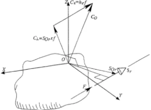
O. The vector C~o is formed by two moment components: a) the moment
component parallel to the screw axis represented byC~k =hrf~; and b) the
moment component normal to the screw axis represented byC~h =S~o×f~
whereS~o, is the position vector of some point in on the screw axis, (see Figure
8). A wrench may be represented by its magnitudeΨrand by a normalized
screwˆ$rthrough
The wrench magnitudeΨ, is the force magnitudekf~k, acting upon
the body, if the action is a pure force, or it is the moment magnitudekC~ok,
if the action is a pure moment. If the action is a force and moment
combina-tion the wrench magnitude iskf~k. Considering a wrench$r = [f ~~ Co]T =
[Lr Mr Nr Pr∗ Q∗r R∗r]T, its corresponding normalized screwˆ$ris defined
by two vectors,[Lr Mr Nr]T. dimensionless~l, and[Pr∗ Q∗r R∗r]T, units of
length~L, so:
ˆ $r=
Lr/Ψr
Mr/Ψr
Nr/Ψr
P∗
r/Ψr
Q∗
r/Ψr
R∗
r/Ψr
= Lr Mr Nr P∗ r Q∗ r R∗ r = ~ Sr ~
SOr×S~r+hrS~r
(2.7)
whereS~r is the normalized vector parallel to the screw axis. It is
important to notice that the vectorS~Or×S~rthe screw axis moment around
the reference system origin.
2.2.2
Reciprocity and rate of work
If a non-null wrench(Ψr6= 0)acts upon a rigid body in such way
that it does not produce work while the body moves around a instantaneous
twist(Ψ 6= 0), both screws (twist and wrench) are calledreciprocal screws
(BALL, 1900; HUNT, 2003).
Figure 8 – Wrench components.
Source: (CAMPOS et al., 2011).
moving around a instantaneous twist$ = [~ω ~Vp] = Ψ ˆ$. Then, the rate of
work or instantaneous power carried out is:
δW =C~ ·ω~n+f~·V~p (2.8)
For convenience, the transpose of a normalized screw is defined in
Plucker axis coordinates (TSAI, 1999), byˆ$T = [P∗ Q∗ R∗ L M N]and
ˆ$T
r = [Pr∗ Q∗r R∗r Lr Mr Nr].
So, the rate of work is:
δW = $Tr$ = $T$r (2.9)
Additionally, the Equation 2.9 may be given by
δW = (ˆ$T rΨ)$r
δW = (ˆ$T
r$r)Ψ⇒
δW
Ψ = ˆ$
T r$r
Table 1 – 6-RUS Robot geometrical parameters.
Symbol Geometric Parameter
rb Radius of the Base
rp Radius of the End-Effector
ri Length of the Crank
Ri Length of the Passive Link
e Half of Distance Between a Pair of Joints (End-effector)
d Half of Distance Between a Pair of Actuators (Base)
χa Angles for Position of Actuators (Base)
χj Angles for Position of a Pair of Joints (End-effector)
β Angles for Actuator’s Orientation (Base)
Source: Own author.
so, the reciprocity condition may be expressed as
δW
Ψ = 0 (2.11)
due a non trivial caseΨ6= 0, the reciprocity condition result in
ˆ $T$
r= 0 (2.12)
2.3
Inverse Kinematic Problem
This section presents a method to solve the Inverse Kinematic
Prob-lem for a 6-RUS parallel robot using some non-physical parameters defined
based on the vectorial equation of the chains.
For the inverse kinematic problem, the vector describing the
end-effector position in cartesian coordinates system and orientation by roll, pitch
and yaw angles, respectively is given byP~ = [Px Py Pz ϕ ϑ ψ].
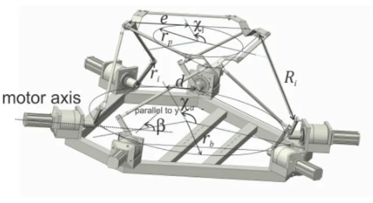
In this method, few geometrical parameters are necessary to develop
obtained from a prototype or a CAD model.
The required parameters are the fixed base radius (rb), the
end-effector radius (rp), the crank dimension (ri) which is located in an active
joint, the passive link dimension (Ri), the half-distance between joints in the
end-effector (e), the half-distance between an active joint pair (d), the position
angle of the actuators pair (χa), the position angle of the passive spherical
joint in end-effector (χj) and the angle between the crank rotational plane and
an axis parallel to y (β). These parameters are detailed in Figure 9.
Figure 9 – Parallel robot geometrical parameters.
Source: Own author.
Initially it is needed to define the position of the actuators, which can
be obtained by Equation 2.13, which must be solved for all limbs, resulting in
a 6x3 vector:
~
A=R~ +m~ (2.13)
Beingi= 1,2,3, ..,6corresponding to each kinematic chain.
~
R=rbcosχaˆi+rbsinχaˆj (2.15)
~
m=−msinχaˆi+mcosχaˆj+ 0ˆk (2.16)
~
A= (rbcosχa−msinχa)ˆi+ (rbsinχa+mcosχa) ˆj+ 0ˆk (2.17)
Similarly, all the platform joint positions, i.e. the spherical joints
attached to the end-effector must be found in the local coordinate system
attached to the base:
~
C=~r+~n (2.18)
n= (−1)i−1
e (2.19)
~r=rpcosχjˆi+rpsinχjˆj+ 0ˆk (2.20)
~n=−nsinχjˆi+ncosχjˆj+ 0ˆk (2.21)
eP C~ =r
The rotational transformation using roll, pitch and yaw angles
nota-tion in (SCIAVICCO; SICILIANO, 1996) is used in order to findeP C~ from
Tool Center Point, attached to end-effector origin eO to spherical joint in
general coordinate system attached to fixed base originbO.
rot=
cϕcθ cϕsϑsψ−sϕcψ cϕsϑcψ+sϕcψ
sϕcθ sϕsϑsψ+sϕcψ sϕsϑcψ−cϕsψ
−sϑ cϑsψ cϑcψ
(2.23)
fP C~ =rotmP C~ (2.24)
In order to find the vector from active joint to spherical joint of a limb
b~I, the vectorial Equation (2.25) must be solved.
bOA~ = bOP~ + bP C~ + bP C~
− b~I (2.25)
b~I= fOA~
− fOP~
− fP C~ (2.26)
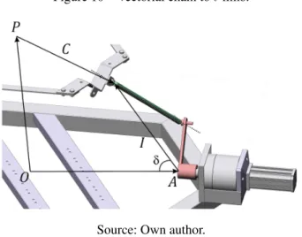
The vectorbI~may be decomposed into two components,I~
ωin the
planeωi, and another one orthogonal toωi.I~ωinωimay be further
decom-posed into two components,I~zandT~, one parallel to thezaxis and contained
in planeωiand another one parallel to thexyplane, respectively.
~
Figure 10 – Vectorial chain toi-limb.
Source: Own author.
The norm of vectorT~ may be written in the components ofbI~terms,
whereIxandIyarebI~components inxandyaxis, respectively.
T = T~
=Ixcosβ+Iysinβ (2.28)
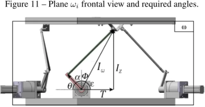
With these definitions, it is possible to analyse the crank rotational
planeωiand define the anglesθ, α, φand ε, which must be found to solve
the inverse kinematic problem, beingθthe crank angle.
An analysis of Figure 11 leads to:
π=ε+φ+α+θ (2.29)
Using the inner product definition and callingM, horizontal
compo-nent ofr~iin planeωi. Where −
~ T
Figure 11 – Planeωifrontal view and required angles.
Source: Own author.
Figure 12 – Planeωifrontal view, geometrical details.
Source: Own author.
~r· −T~ =k~rk
~ T
cosθ (2.30)
−Tˆ= ˆr (2.31)
~
M =k~rkcosθ (2.33)
Multiplying by2T both sides.
2T M = 2Tk~rkcosθ (2.34)
A non-physical parameteruis defined which allows to re-write
Equa-tion 2.34 as:
u= 2T ri (2.35)
u=2T M
cosθ (2.36)
Using same method, another non-physical parameterv is defined,
however the equation is multiplied by2Iz. WhereNis the vertical component
ofr~iand the formulation is similar toM.
v=−2Izk~rk (2.37)
~r·Iz=k~rk
I~z
cosα (2.38)
N =k~rkcosα (2.39)
v=2IzN
cosα (2.41)
In these terms is it possible to define the relation between u
v and
determine the angleφ.
φ= arctan T
Iz
(2.42)
u v =
2T Mcosα
2IzNcosθ
(2.43)
M N =
cosθ
cosα (2.44)
u v =−
T Iz
(2.45)
φ=−arctanu
v (2.46)
It is not necessary to use this method to findφonceIz andT are
known. However, since the parametersuandvwill be used in afterwards, it is
convenient to show the formulation.
An analogous method is applied in order to find other relations to
solve the inverse kinematic problem. Callingsthe projection ofIωoverr~iand
multiplying by2rifor convenience.
s= ~ Iω
Figure 13 – Planeωifrontal view.
Source: Own author.
2ris= 2ri
I~ω
cos (φ+α) (2.48)
Using the closed-loop equation leads to:
R~ 2 = I~ 2
+k~rk2− I~
k~rkcosδ (2.49)
Beingδthe real angle crank and vector I~. Analyzing Equation 2.49
in crank rotational plane, it is possible to affirm thatδ=α+φ, and then the
non-physical parameter,wis defined.
w=−2k~rk I~ω
w=R2 i − ~I −r 2 i (2.51)
Also, manipulating the geometrical equations of the triangle rectangle
showed in Figure 13, it turns out that.
s2
=
−w
2ri
2
(2.52)
u2
+v2
= (2T ri)
2
+ (−2Izri)
2
(2.53)
u2
+v2
= (2ri)
2
(Iω)
2
(2.54)
From the triangle rectangle showed in Figure 13
z2
+s2
=
I~ω
2
(2.55)
(2ri)
2 z2
+ (2ri)
2 s2
= (2ri)
2
I~ω
2
(2.56)
Then another non-physical parameterq, is defined and Equation 2.56
is re-written as.
q= 2riz (2.57)
q2
+ (2ri)
2 s2
= (2ri)
Substituting Equation 2.52 into Equation 2.58:
q2
+w2
= (2ri)
2
I~ω
2 (2.59) q2
= (2ri)
2 ~ Iω 2 − ~ Iω 2
cos (φ+α)
(2.60)
q2
= (2ri)
2
I~ω
2
sin (φ+α) (2.61)
q2 w2 =
(2k~rk)2 I~ω
2
cos2
(φ+α)
(2k~rk)2 I~ω
2
sin2
(φ+α)
(2.62)
tan (φ+α) = q
w (2.63)
φ+α= arctan q
w (2.64)
Returning to Equation 2.29.
π=ε+φ+α+θ
ε=π
2 −φ (2.65)
π=π
2 −φ
θ=π
2 +φ−(φ+α) (2.67)
θ=π
2 −arctan
u
v −arctan
q
w (2.68)
With these definitions, the inverse kinematic problem is solved. Once
functionarctanhas a dubious response, it is convenient to usearctanwith
two arguments (atan2 function).
An algorithm that compute the joint and actuators position and
com-pute the parameteru,v,wandqas presented solve the inverse kinematic
problem using really low computational coast.
For convenience Equations 2.35, 2.37, 2.51, 2.59 and 2.54 may be
re-written to computeu,v,wandqbased in previously values and apply in
2.68.
u= 2ri(Ixcosβ+Iysinβ) (2.69)
v=−2riIz (2.70)
w=R2
i −r
2
i −I
2
x−I
2
y−I
2
z (2.71)
q=pu2+v2−w2 (2.73)
The same algorithm is useful to find the workspace to a given
ori-entation using some increments toPx, Py and Pz and solving the Inverse
Kinematic Problem repeatedly it is possible to find the workspace of the
3 ROBOT SINGULARITIES
The kinematics study of mechanical systems leads inevitably to the
singular configurations problem. They correspond to configurations of the
sys-tem that are usually undesirable since the degree of freedom is instantaneously
changed. These special configurations are defined as the ones in which the
Jacobian matrix, i.e., the matrix relating the input rates to the output rates,
becomes rank deficient (GOSSELIN, 1988).
In this section it is present a differential kinematic relation for parallel
manipulators and introduce their singularities. This differential kinematics is
based on the parallel manipulator Jacobian matrix.
In spatial parallel manipulators, the relationship between actuator
coordinate vectorqand end-effector Cartesian coordinate vectorP, may be
stated as a functionf
f(θ, P) = 0 (3.1)
where 0 is the 6-dimensional null vector, Therefore, the differential kinematic
relation may be determined (TSAI, 1999)
Jqθ˙−Jx$ = 0
Jqθ˙=Jx$
˙
θ=J$
(3.2)
where $ is the end-effector velocity in ray order,θ˙ = [Ψ1, ...,Ψl] is the
input twist magnitude vector andJ =J−1
q Jxis the Jacobian matrix of the
manipulator composed by directJx, and inverseJq Jacobian matrices.
relation-ship between the end-effector velocity $ and the vectorυ = [υ1, ..., υn]T
υ=Jx$ (3.3)
whereυis the component of the absolute linear velocity of the end-effector
connection point in the direction of the passive link,i.e.the distal link of
each limb (serial chain between basis and end-effector) (DAVIDSON; HUNT,
2004a),e.g.in the 6-RUS parallel robot of Figure 14, the connection point is
Ciand the passive link isBiCi.
Figure 14 – Position of pointsB, andC.
Source: (MERLET, 2000).
Singular configurations occur if eitherJx orJq is singular. If Jq
is singular, alimborinverse kinematicssingularity is encountered and
end-effector is over constrained (TSAI, 1999),i.e.it instantaneously loses at least
one degree of freedom.. Using equation 3.4, there is a inverse kinematic
zero output,$ = 0. In this case:
Jqθ˙= 0 (3.4)
In other words, this type of singularities consists of the set ofpoints
where different branches of the inverse kinematic problem meet, the inverse
kinematic problem being understood here as the computation of values of the
input variables from given values of output variables(GOSSELIN, 1988).
The inverse kinematic singularity is found, typically, at the boundary
of the workspace or when the limbs folds upon itself. This type of singularity
is caused due the serial nature of the limbs and is discussed extensively in
literature (SCIAVICCO; SICILIANO, 1996; TSAI, 1999).
IfJxis singular, a platform or direct kinematic singularity is
encoun-tered and the end-effector can move instantaneously even if all actuators are
locked. At these configurations, the manipulator gains one or more
uncon-trollable degrees of freedom at the end-effector. For instance, there exists a
non-zero output velocity,$, corresponding to a zero input velocity,θ˙,i.e.
0 =Jx$ (3.5)
This corresponds to configurations in which the chain remains
uncon-trollable even when all the actuated joints are locked. As opposed to first one,
this type of singularity lies within the workspace of the chain and corresponds
to apoint or set of points where different branches of the direct kinematic
problem meet. The direct kinematic problem is the one in which it is desired
variables. Since the nullspace ofJ is not empty, there exists a set of output
rate vectorsx˙which will be mapped into the origin byJ, i.e., which will
cor-respond to a velocity of zero of the input joints. The input rates area therefore
not independent (GOSSELIN, 1988). This type of singularity occurs within
the workspace and is the main goal of this report.
A third type of singularity happens when bothJxandJqare singular.
This situation was first inadvertently classified as dependent on a certain
special design of the manipulator, but was later proven incorrect (DANIALI;
ZSOMBOR-MURRAY; ANGELES, 1995) by way of examples that the third
type of singularity does not occur only in “special” mechanism. Rather. it can
occur in "regular" mechanism.
In general inverse kinematic singularities are easier to detect and
move outside of the desired workspace by changing limb lengths. However.
since direct kinematic singularities happen within the workspace, they
effec-tively partition the workspace into smaller usable portions.
There are three basic reasons why direct singularities become an issue
in real life situations. They follow directly from the interpretations of
singular-ities and are: reduced accuracy, large internal forces and loss of knowledge of
solution tree (VOGLEWEDE, 2004).
•Degenerate accuracy. The JacobianJ(J =−J−1
q Jx) (TSAI, 1999)
analysis relates the input and output velocities. At direct singularity the
end-effector can have an instantaneous velocity at the output for zero input velocity.
becomes
˙
θ=J$
∆θ
∆t ≈J
∆X
∆t
∆θ≈J∆X
(3.6)
Therefore, theoretically, when the manipulator is at a direct singular pose, the
end-effector only has a very small instantaneous motion,i.e.no motion at
all. However, in practice, all manipulators have some amount of clearances
(and similarly some compliance) and allow some finite motion at the
end-effector. This motion is denoted as the unconstrained end-effector motion. The
problem is to find out how much unconstrained end-effector motion is allowed.
•Large internal forces. The direct kinematic singularities affect the
internal forces,i.e.the static forces required by the actuators (input forces)
approach to infinity at singularities.
•Solution tree. The solutions for the forward kinematics coincide
at direct singularities. In practice the two different solutions cause control
problems. If the manipulator moves close to a singularity and slips into the
other solution due to overshoot, the manipulator mechanically is not where
the control believes it is. The manipulator will be at a different end-effector
position than predicted and could lead the manipulator into poses where it was
3.1
Direct Singularity
Direct singularities may be introduced studying the mechanical
equi-librium of a parallel robot. Consider the input articular torque/force vector
τ= [Ψr1, ...,Ψr6],i.e.the input wrench magnitude vector. If a wrench$ris applied on the end-effector, the mechanical system will be in equilibrium, if
the resultant of the articular forces($r1, ...,$r6)which act on the platform
is equal and opposite to the$r, if not the end-effector will move to reach an
equilibrium position. In an equilibrium position there is a relation betweenτ
and$r(DAVIDSON; HUNT, 2004b)
JT
xτ = $r (3.7)
where the columns ofJT
x are the normalized screws (axial order) representing
the wrenches acting on the end-effector(end-effector), i.e.the Plucker vector
coordinates of the actuating force lines (MERLET, 2000; TSAI, 1999).
JxT =
Lr1 ... Lr6 Mr1 ... Mr6 Nr1 ... Nr6 P∗
r1 ... Pr∗6 Q∗
r1 ... Q∗r6 R∗
r1 ... R∗r6
= ˆ
$r1 ... ˆ$r6
τ (3.8)
The quantity$r, is at wrench screw representing the action supported
by the body, in ray coordinates. From this equation, it is seen that not only
input to static forces and moments. Therefore, there is another interpretation
of singularities.
Figure (15a) shows the wrenches acting upon the end-effector. Two
examples of possible direct singularities are shown in Figure (15b) and (15c),
these are two cases previewed by Grassmann analysis that are inside the robot
workspace.
Figure 15 – (a) The wrenches acting upon the end-effector. (b) and (c) Two direct singularities.
Source: (CAMPOS; GUENTHER; MARTINS, 2005).
Direct kinematic singularities occur when there exists a
force/mo-ment, in the end-effector, in one or more directions that cannot be resisted by
the inputs. When all the forces, acting up on the end-effector, intersect a one
point the manipulator cannot resist a moment around that point. This point
may be infinity and in this case the forces are parallel and they cannot resist a
perpendicular force acting on the end-effector.
3.1.1
Singularity detection method
Singular configurations rest on the singularities of the Jacobian
ma-trix. Singularities correspond to the roots of Jacobian determinant. However,
e.g.Maxima (www.gnu.org.software/maxima/maxima.html), is a complicated
labour for general robots (MERLET, 2000). After the calculating, of the
de-terminant it is necessary to find its roots within the workspace which is a
even more difficult task because the determinant in general is a non linear
ex-pression. This method is useful only tor particular parallel robots (DANIALI;
ZSOMBOR-MURRAY; ANGELES, 1995; TAHMASEBI, 1992).
Some researchers analyse intuitively some particular cases of
singu-larity for the Jacobian matrix and have obtained certain cases of singusingu-larity
(FICHTER, 1986), (HUNT, 1978), (LIU et al., 1993). Geometric method,
based on Grassmann geometry, solve the problem for many different robots
(MERLET, 2000). There are other methods which use a special variable to
"measure" how "far" a pose is from a singular, for instance thecondition
numberof the Jacobian matrix (XU; KOHLI; WENG, 1994). In this section,
the geometric method and the closeness to singularity measures are presented.
3.1.2
Grassmann Geometry
Equation 3.8 is a linear system of equations in term of articular force
τ. If the system is rigid, this means that for any action $r(force moment) up
on the end-effector, there exists one set of articular forcesτ (or moments)
such that the system is in an equilibrium state. This relation only is possible
if matrixJT
x is of full rank, i.e. the Plucker vectors (columns ofJxT) are
linearly independent. So,a singular configuration of a parallel manipulator
corresponds to a configuration where it is no rigid.
In most cases the wrenches acting upon the parallel manipulator
cor-respond to a Plucker components of a line.i.e.a Plucker vector. In these cases,
the singular configurations of the manipulator are associated with linearly
de-pendent set of lines, also called line based singularities (HAO; MCCARTHY,
1998). Grassmann studied the varieties of lines. i.e. the sets of linear
depen-dent lines tongiven independent lines, and characterised them geometrically
(MERLET, 1989).
These varieties were analysed and classified in order to study the
singularities of spatial frameworks (DANDURAND, 1984) and triangular
simplified symmetric manipulator whose six limbs connect to the end-effector
and to the basis only in three points, respectively (MERLET, 2000)(HAO;
MCCARTHY, 1998).
The linear system of equations Equation (4.7) represents a rigid
system if for any action$r upon the end-effector, it is possible to find a
set of input wrench magnitudesFi. This condition is only feasible when
matrixJT
x is full rank,i.e.the Plucker vectors (columns ofJxT) are linearly
independent. So a singular configuration of a parallel manipulator corresponds
to a configuration where it is not rigid.
The linear varieties are classified according to its rank (MERLET,
1989)(see Figure 16):
•The zero rank set is empty.
•The variety of rank one contains a line in the 3D space. The variety
Figure 16 – Grassmann varieties of dimension 1,2,3,4,5,6.
Source: (MERLET, 2000).
have no intersection and are not parallel (also called agonic lines), or a flat
pencil of lines,i.e.lines in a plane which intersect in one point.
•The variety of rank three is of four types: a regulus 3a, two flat
pencil of lines in different planes and with different centres 3b, a bundle of
•The varieties of rank four, called linear congruences, are of four cases: elliptic, hyperbolic, parabolic and degenerated congruence, details in
(HUNT, 1990; MERLET, 1989).
• Linear varieties of rank five, called linear complex, are of two
types: nonsingular (or general): generated by 5 independent skew lines 5a,
the complex is the set of lines tangent to coaxial helices; and singular (or
special): all the lines meeting one given line 5b, this case is subdivided
de-pending on if this line is at infinity 5b2 or not 5b1 (HAO; MCCARTHY, 1998).
Therefore, if the Plucker vectors, lines in the direction of the forces
acting upon the end-effector, are in any of the above varieties (rank= 1, ..., 5),
the parallel manipulator is in a direct singular configuration.
3.2
Singularity Closeness Measures
In this section some methods to measure the closeness of the
singu-larity are presented based on the Voglewede thesis (VOGLEWEDE, 2004).
Initially, the criteria of measure must to beframe invariant, scale
invariant and unit invariant:
•Frame invariant. A quantity that does not change due to a change of the coordinate system’s location or orientation is said to be frame invariant.
units of the coordinate frame (e.g.meters or inches) is said to be unit invariant.
•Scale invariant. A quantity does not change due to a change of the size (or scaling) of the manipulator is said to be scale invariant.
3.2.1
Linear Algebra Based Measures
Mathematically, singularities are defined where the Jacobian
relation-ship degenerates. Therefore, the most obvious method to evaluate singularities
is to use techniques from linear algebra.
Condition number
The condition number was first suggested by Yoshikawa (YOSHIKAWA,
1990) as a local measure or how close one is to singularity. The condition
number is defined as
k= σmin
σmax
(3.9)
whereσminandσmaxare the minimum and the maximum singular values of
the Jacobian matrix, J. This measure is not frame or unit invariant if the entries
of the Jacobian matrix are not uniform (LIPKIN; DUFFY, 1988; DUFFY,
1990).
Jacobian Determinant
Another possible measure to know how close one is to a singularity is
the determinant of the Jacobian matrix. It is proved that the determinant of the
However, the geometric meaning of the determinant is not clear,i.e.we do not
know what is a “good” value for determinant. Additionally, in general, finding
a physical meaning for the determinant is very difficult (VOGLEWEDE,
2004).
3.2.2
Screw Theory Based Measures
Screws are briefly introduced in Chapter 2. This analysis decomposes
all instantaneous rigid body motion into a rotation around an axis and a
translation along the same axis,i.e.a twist. A dualism of this concept is that
all forces acting on a rigid body can be decomposed as a force along an axis
and a moment around that axis,i.e.a wrench.
Using the screw theory, specifically the rate of work presented in
Section 2.2.2 a technique was developed to determine how close one is to a
singularity (POTTMANN; PETERNELL; RAVANI, 1998). The rate of work
or power product is defined as the normal dot product between a wrench$r,
represented in axis coordinates, and a twist$, represented in ray coordinates,
or vice versa, see Equation 2.8 here repeated.
δW = $T
r$ = $T$r=C·ωn+f·Vp (3.10)
whereδWis the instantaneous power between the force and the twist. Porttman
et al.determine the twist that minimize the square of the power (to keep two
different power calculations from canceling out) with all the rows of the
Jacobian (i.e.the wrenches). This based power calculation is used as a measure
to see how close one is to a singularity. In other words, they find the twist
the power product, Equation 3.10. This approach is used for a linear complex
approximation technique to measure the closeness to singularities (WOLF;
4 SINGULARITY POWER INSPIRED MEASURE
This chapter determines closeness to singularities by formulating the
question in terms of a constrained optimization problem. The constrained
opti-mization problem results in a corresponding generalised eigenvalue problem.
The resulting eigenvalue has physical meaning and is utilized as a measure
of the performance near singularities, and thus is a measure of closeness to
singularities.
This optimization approach was used to the singularity analysis.
Pottman et al.(POTTMANN; PETERNELL; RAVANI, 1998) use the
con-strained optimization problem to determine the linear complex that is closest
to a singularity. Wolf and Shoham (WOLF; SHOHAM, 2003a) use the
method-ology to describe the instantaneous behaviour near singularities. Voglewede
(VOGLEWEDE, 2004) incorporate several other seemingly non-related
mea-sures into the constrained optimization framework, for instance the natural
frequency measure.
4.1
Minimization Problem
Accordingly Voglewede (VOGLEWEDE, 2004), a measure of
close-ness to singularitiesM(X), at a particular configuration,X,i.e.position and
orientation,
M :{conf iguration space} → ℜ
M :{X} → ℜ
should have the following three properties:
•M(X) = 0if and only ifXis a singular configuration,
•IfXis non-singular,M(X)>0, and
•M(X)has clear physical meaning.
If one approaches the problem of creating a measure from a physical
standpoint, one first need to define the physical quantity,M(X), one cares
about. As shown above, a singular configuration has many different effects,
including loss of constraint, increased end-effector error, loss of stiffness
and degenerated actuator torque transmission. The effect that we are most
concerned about is the loss of constraint so it forms the basis of the singularity
measure.
In this case, if one cares primarily about the loss of constraint that
occurs in at least one direction at a singular configuration, an appropriate
measure that also applies to non-singular configurations is the amount of
constraint provided by the mechanism in the least constrained direction. In this
case, the physical quantity of interest at configurationXfor twist direction $
is obtained by minimizingFover all "unity" motions, $, as follows:
M(X) =
min F(X)
subject to k$k2=c
(4.2)
wherek...krepresents a type of norm for twists (several norms may be found
in (VOGLEWEDE, 2004) andcis a constant. The twist is constrained to have
a certain norm because otherwise the trivial solution,$ = 0, would always be
the minimum.
So it is necessary to obtain an objective functionFand an appropriate
normalization of$for minimization the problem of Equation 4.2.
4.1.1
Twist Normalization: Invariant Norm
The general minimization problem presented in Equation 4.2 requires
normalization a of a twist, which raises many issues on how this vector
should be normalized, due the different dimension terms in the vector (twist)
components. Specifically, we chose the invariant norm of the twist, other most
used common norms are the Euclidean norm and the kinetic energy norm
(VOGLEWEDE, 2004).
Theinvariant normtakes the magnitude of only the frame-invariant
given twist: $ = ω Vp (4.3)
the invariants norm is
k$k=√ω·ω=p$TD$ (4.4)
where
D=
I3x3 03x3
03x3 03x3
(4.5)
It is important to notice that ifω = 0, the invariant norm becomes
null, therefore for the case of pure translation the invariant norm must be
supplemented, for instance a potential solution is (VOGLEWEDE, 2004):
If ω= 0, thenk$k=p
Vp·Vp (4.6)
and in this case
D=
03x3 03x3
03x3 I3x3
(4.7)
The invariant norm of Equation 4.4 deals well with finite pitch twists
(h6=∞),i.e.twists withω6= 0.
4.1.2
Objective function: power inspired measure
A objective function which results of the power inspired measure is
1998; WOLF; SHOHAM, 2003b)
F($) =
k
X
i=1
(ˆ$T ri$)
2 (4.8)
hereˆ$riare the columns, in axial order, ofJxT, see Equation 3.8 that,
particu-larly, can be interpreted as unitary magnitude wrenchesˆ$ri∼= $ri, andkis the
number of rows. The motivation for this measure, using parallel manipulators,
comes from the dual meaning of the Jacobian matrix. Namely, columns of
JT
x may be interpreted as the (normalized) wrenches applied by the limbs
(specifically by passive links) for unit actuator torques and each term(ˆ$T
ri$)
2
ofFmay be interpreted as the square of the power e.g.
N2 m
2/seg2of the
ith limb on the end-effector twist,$. Strictly, given thatˆ$ri, is a normalized
screw and is not a unitary magnitude wrench, the magnitude ofFisL/T2e.g.
[m/seg]because, see Equation 3.3.
ˆ$T
ri·$ = [Pri∗Q∗riR∗riLriMriNri]·[Lr,Mr,Nr,(P∗,Q∗,R∗)]T
= F
= (Jx$)T(Jx$)
= υTυ
= kυk2
(4.9)
In a singular configuration there exist a twist$for which none of the
limb actions can do any work and thus the minimum ofFgoes to zero. Away
from singular configuration, the minimization identifies theleast constrained
twist- with the restriction that its angular part be of norm one - and uses the
Rearranging Equation 4.8 in the form or Equation 4.2, this measure
becomes:
M(X) =
min F($) = $TJT
xJx$ = $TM$
subject to g($) = $TD$
−c= 0
(4.10)
whereM (also called Graminiam matrix) andDaren×nsymmetric positive
semi-definite matrices,gis a given constraint, andcis some positive
con-stant (VOGLEWEDE, 2004), thereforeFonly takes on non-negative values,
F($)≥0.
We want to minimize the functionF subject to given constraint. In
other words, into the set of values of $ that satisfy the constraint, we want to
find the ones that give the minimum valueF.
All possible constraints for a two variable function, can be rearranged
to readg(x, y) = 0. For instance, the constraintx2y = 3may he written as
x2y
−3 = 0and so forth. The equationg(x, y) = 0give us a line or curve
in thexy plane. We want to go along that line and find the point on with
the largest value ofF (in this exampleF(x, y)). When we find the largest
value, we know thatF(x, y)will be stationary as we move along the line.
That is what a minimum (or maximum) means. This in turn means that the
gradient∇Fis perpendicular to the line of the constraint at this point, because
the gradient is always perpendicular to the contour. But the constraint is also
constant along the line, it is zero by construction. So it also has a gradient∇g
do point in the same direction. In other words, they are proportional to each
other∇F =λ∇g, whereλis some number that we do not at present know
the value of. This numberλis called aLagrange multiplier. Rearranging we
see that∇F−λ∇g= 0, or if given that:
¯
F(x, y) =F(x, y)−λg(x, y)then∇F¯= 0 (4.11)
If∇F¯= 0, the all partial derivatives ofF¯are zero. This give us a method to
finding our minimum. We simply construct the functionF¯(x, y)as above, but
multiplyinggby a constantλ, then we set all partial derivatives ofF¯(x, y)
to zero and solve the set of simultaneous equations we get. This give us a
solution for the minimum ofF¯.
The only problem is that the solution still contains the constantλ,
whose value we do not know. But we can solve that problem easily enough.
We still have one more equation - the constraint. If we substitute our solution
forxandyback into the constraint, we get another equation that we can solve
forλ.
It is possible to show that the method generalizes to more than two
variables and more than one constraint. If we have a set{xi}, o= 1, ..., nof
variables and setgj({xi}), j= 1, ..., mof constraints, then one constructs the
function
¯
F(xi) =F(xi)− m
X
j=1
λjgj(xi) (4.12)