Abstract
The effects of distinctive parameters such as revolute joint angle or spherical joint location of mobile platform in a 6-DOF 6-RUS parallel manipulators on workspace, kinematic, and dynamic indi-ces are investigated in this study to select proper structure com-mensurate with performance. Intelligent multi-objective optimiza-tion method is used to design the manipulator. Considering dis-tinctive parameters, relevant relations for developing inverse kin-ematic and Jacobin matrix are obtained. In order to study dynam-ic properties, mass matrix is obtained from calculating the total kinetic energy of the manipulator. After modifying multi-objective Bees algorithm, it used to optimize the manipulator structure considering all geometrical parameters with proper constraints. In addition of comparison of three well known 6-RUS manipulators’ types, variation diagram of workspace, local and global dynamics and kinematics performance indices have been drawn with respect to structural parameters variation and limitation of these parame-ters with proper value are determined. Moreover, considering all dimensionalparameters, Pareto front line of multi objective opti-mization of structure is presented based on dynamic and kinemat-ic performance in pre-determined workspace. Based on the results, a fairly comparison among various types of 6-RUS manipulators can be conducted and the most appropriate set of dimensional parameters are selected based on specific demand.
Keywords
6-RUS parallel manipulators, Structure comparison, performance indices, optimization, multi-objective Bees algorithm.
Structure Comparison and Optimal Design of 6-RUS Parallel
Manipulator Based on Kinematic and Dynamic Performances
1 INTRODUCTION
Parallel manipulators are increasingly used in various industrial applications for their high capacity of load carrying, good dynamical properties, and high precision in positioning. These manipulators
Erfan Mirshekaria Afshin Ghanbarzadehb Kourosh Heidari Shirazi c
a,b,c Mechanical Engineering Department,
Shahid Chamran University, Ahvaz, Iran
corresponding author:
b [email protected] c [email protected]
http://dx.doi.org/10.1590/1679-78252937
are made of mobile platform which is connected to a fixed platform by several parallel arms. Paral-lel manipulators can be classified based on degree of freedom, number of arms, order of joints in each arm and type of actuator (Merlet, 2006). according to this, various 6-DOF parallel manipula-tors have been proposed. One of the most important 6-DOF parallel manipulamanipula-tors is 6-RUS ma-nipulators that revolute joint, universal joint, and spherical joint are used in each arm, respectively. A 6-RUS manipulators has some advantages that the most important one, is low weight of movable parts because of installing motor in the fixed platform. Therefore, bigger and cheaper elec-trical motors can be used. In addition, thinner connecting rod can be used to the mobile platform that conclude reduction of collision of links to each other (Bonev, 2002). Moreover, these manipula-tors can be balanced statically (Gosselin and Wang, 2000). Although this type of manipulator has some disadvantages such as bending in connecting rods and complicated mechanical analysis. Also, because of great number of chains, connecting the fixed base with the moving platform, and movment limitations of passive joints, such as spherical and universal, workspace of the 6-RUS ma-nipulators are restericted. To overcome such drawbacks, some researchers demonstrate the tendency for the use less than 6-degree-of-freedom parallel mechanisms (Chablat and Wenger, 2003; Gosselin
et al., 2007; Clavel, 1991) and for 6-dof applications hybrid manipulators are studied (Caro et al., 2015).
The first 6-RUS manipulator was proposed by Hunt(1983). Kinematics and dynamics of Hunt type manipulator was examined by Gil et al.(2004). Moreover, Aginaga et al.(2012), improved static stiffness of this manipulator using inverse singularities. Another type of 6-RUS manipulators is Hexa that proposed by Pierrot(1990) based on 3 DOF delta (Clavel, 1988). This manipulator has same advantages of Delta manipulator, such as high velocity and high acceleration and in addition it has three rotary DOF. The first model of this manipulator was made by Uchiyama (1993) and the di-rect kinematic of Hexa was developed by Hesselbach et al.(2005). Moreover, calibration of this ma-nipulator was conducted by Dehghani et al.(2014). Another arrangement of 6-RUS mama-nipulator was proposed according to the required performance by various references such as proposed manipula-tors by Zamanov (Merlet, 2006)), Takeda et al.(1997) and Campos et al.(2013). In addition, various types of this manipulator with industrial application were proposed by Servos & Simulation Inc. (Merlet, 2006). All mentioned types have the same topology but they are different according to the revolute joint axis angle and the connection point to the fixed platform. Generally, few studies have been done on the RUS structures rather than other DOF manipulators such as UPS and 6-PUS (6-DOF manipulators with linear actuators).
In order to compare all structures, some criteria are presented to evaluate manipulators perfor-mance. These criteria can be classified to kinematic-static criteria (Cui et al., 2014; Rezaei and Akbarzadeh, 2015) such as isotropy, manipulability, dexterity, workspace and singularity, and dy-namic criteria (Nguyen et al., 2015; Zhao, 2013) such as dydy-namic isotropy, dydy-namic dexterity and natural frequency. Depending on extensive application of these manipulators, one or more criteria are required to mention.
have diverse relationships. Another issue is that there are no direct relationships between the per-formance specifications and the structural parameters and solving the optimization problems will have several responses (Khan and Angeles, 2006).
Hence, it is seen by studying the available references that in spite of great applications of 6-RUS parallel manipulators and proposed new various types by researches, structural difference be-tween all manipulators and comparing their performances haven’t been examined yet and no guid-ance has been proposed to select the proper dimensional parameters based on desired application. moreover, Although, a simplified type of 6-RUS manipulator in Liu et al.(2002) has been examined based on kinematic dexterity index, no reference was seen to examine this manipulator based on dynamic index. In addition, multi-objective optimization problems of 6-RUS manipulator were not mentioned especially if dynamical performance included.
Three samples of the most well-known 6-RUS group manipulators are classified in this research after determination distinctive parameters. Dynamic and kinematic performance indices are pro-posed to examine performance and effect of structure variation on performance criteria. In addition, 6-RUS manipulator structure is optimized by using the modified multi objective Bees Algorithm(Pham and Ghanbarzadeh, 2007).
2 DESCRIPTION OF NOTATION FOR 6-RUS
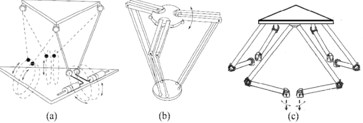
Three 6-RUS manipulators include Hunt type (Hunt, 1983), Hexa (Pierrot, 1990) and a manipula-tor named Zamanov type by the authors as it was proposed by Zamanov (Merlet, 2006) are shown in Figure 1.
Figure 1: 6-RUS parallel manipulators (a): Hunt type (b): Hexa (c): Zamanov type.
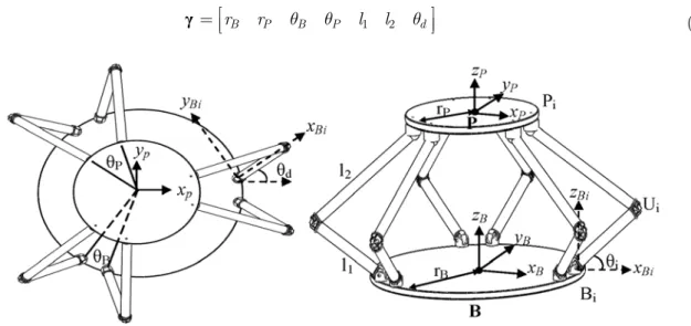
Schematic of a manipulator is shown in Figure 2 to determine different aspects. According to the Figure 2, B and P are center of coordinate connected to fixed and mobile platform, respectively. Revolute, universal, and spherical joints in branch i are shown as Bi, Ui, and Pi, respectively. length
of Each arm is l1 and connecting rod length is l2. Moreover, radiuses of fixed and mobile platforms are rB and rP, respectively. qd is angle between BBi and image of line UiPi on fixed platform.
Angles between joints on fixed and mobile platforms are qB and qP, respectively. As it is observed,
1 2
B P B P d
r r q q l l q
é ù
= êë úû
γ (1)
Figure 2: Geometrical parameters of 6-RUS parallel manipulator.
According to Figure 1,with neglecting dimensional differences, the main difference in 6-RUS manipulators has two cases; first is how to place two arms beside each other which is result of dif-ference in revolute angle qd. For example, in Hexa and Hunt type manipulators, arms next to each
other move in two parallel platforms but in Zamanov type manipulator, arms move in a plain against each other. The second parameter is the position of spherical joints on mobile platform qP.
Examining other parameters shows that change in parameters size doesn’t change in manipulator structure so these two parameters are considered as distinctive parameters. To clarify this issue, structural parameters values for three manipulators are shown in Table 1; therefore, each structure can be introduced by relevant qd and qP.
d
q
P
q Manipulator Type link
0
-1
2 sin ( sin( )) 2
B B
P
r r
q Hexa
0 120
Hunt
90 0
Zamanov
Table 1: Structural parameters of 6-RUS parallel manipulators.
3 CRITERIA OF PERFORMANCE EVALUATION
3.1 Workspace
Workspace is the most important criteria in selecting structure particularly when a manipulator wants to transfer and move objects. Manipulator workspace is collection of all configurations that end-effector can obtain it by proper selection of joints coordinates. Generally, workspace is limited in parallel manipulators, hence this factor is the most important factor in design. Numerical ods (such as discretization (Rezaei et al., 2013), and analytical methods (such as geometrical meth-ods (Bonev, 2002) have been studied. Calculating workspace for 6-RUS fixed manipulator is pro-posed using geometrical method (Bonev, 2002); however, this method can not be used for reachable workspace.
In this way, discretization method is used to extract workspace. In the mentioned method, space is divided to small distinct spaces then corresponding joint angles to various points are ob-tained by inverse kinematic. If obob-tained angles are not in permitted range, that point will belong to workspace.
Workspace of the manipulator may has an irregular shape. However, in some applications, regu-lar workspace shape such as cubic shape workspace is required. In such cases, the biggest volume cubic shape inscribed in the reachable workspace is extracted. In the current study, a procedure described by Hosseini et al. (2011) is used to obtain the maximal inscribed cubic workspace.
3.2 Kinematic Performance Indices
One of the important criterion to evaluate kinematic performance for parallel manipulators is dex-terity. Dexterity is end-effector ability of very small volunteering precise and easy movements around a point in workspace. Therefore, manipulator can perform highly precisely if they have high dexterity and are proper to be used in precise location and simulation. To calculate manipulator dexterity, Jacobin matrix is needed to relate end-effector velocity vector X and actuated joints velocity vector q as the relation 2.
q = J X (2)
Many indices are used to estimate parallel manipulator kinematic dexterity which important ones are condition number and manipulability indices. Condition number shows relation of the ex-isted error in operating joints and end-effector error in Cartesian space. Jacobin matrix condition number is obtained by:
-1 =
kJ J J (3)
Condition number based on Jacobin singular values may be written as relation (4). max
min ( ) =
( )
k s
s J
J
J (4)
In which smax( )J and smin( )J are maximum and minimum eigenvalues of the Jacobian matrix.
dex-terity of the manipulator. LCI varies from 0 to 1, which o shows the ill situation and 1 indicates good situation.
Of course, the mentioned indices have some problems in dimension and physical interpretation (Khan and Angeles, 2006), because Jacobin matrix elements have similar dimension. Some methods are proposed to solve these problems. One of the most applied method is that Jacobin matrix di-vides to two translational and rotational coefficients parts and condition number of each one is ob-tained.
Another applicable method is using of part of Jacobin matrix with length dimension that is di-vided to coefficient with dimension. This coefficient is stated variedly in different references. For example, in a reference based on one of structural parameters, manipulator is as a platform radius. However, what is stated in this article is characteristic length that is said in Fassi et al.(2005) based on Jacobin matrix properties. In this regard, characteristic length is stated as equation (5).
trace( )
=
trace( )
T R R
c T
T T
L J J
J J (5)
Where JR and JTare translational and rotational parts of Jacobin matrix, matrices size is 3*6.
By using this coefficient, homogenized jacobian matrix are expressed as:
[ R]
T c
L
= J
J J (6)
The proposed indices for measuring manipulator dexterity is depending on manipulator condi-tion, so global conditioning index (GCI) can be used as equation (7).
W
1 1
= =
dW
W W
dW dW
k k
W
h
ò
ò
ò
J J
J (7)
3.3 Dynamic Performance Indices
Dynamics examines relation between velocity and acceleration the end-effector with inserted forces and torques on joints. This relation is stated by a series of differential equations that are movement equations. Dynamic equations dominant on manipulator can be expressed by equation (8).
( ) + ( , )+ ( )=
M q q C q q G q t (8)
In which M q( ) is inertia matrix, C q q( , ) is Coriolis and centrifuge parts matrices, G q( ) is mass matrix, and t is inserted torque matrix on joints. Dynamic relations has principal role in some applications such as manipulators with high velocity, high load carrying capacity, high pass band manipulators, and high performance manipulators.
Hence, proper criteria should be used to be perceived simply by designer to insert necessary changes to improve system dynamic. Therefore, some indices are used to estimate dynamic performance.
The initial methods to describe dynamic specifications proposed by Asada(1984) which exam-ined the relation between generalized manipulator speed and generalized inertia ellipsoid method (GIE). Khatib(1995) presented belted inertia ellipsoid method (BIE) based on (GIE) and analyzed redundant manipulator dynamically using this method.
Dynamic dexterity is one of the important parameters in manipulators, dynamic dexterity states ability of accelerating of end-effector in each point in any desirable direction in manipulator specific condition (Wu et al. 2008). For example, one of the useful indices to show manipulator dy-namic dexterity is Yoshikawa (1985) dydy-namic manipulability. Yoshikawa investigated the relation-ship between generalized accelerations and forces and proposed dynamic manipulability ellipsoid (DME) ability.
In this part, dynamic dexterity is used as dynamic performance investigation criterion. Dynamic dexterity index is extracted by equation (9).
max
min
( )
=
( )
T T
k s
s M
J MJ
J MJ (9)
1/kM is considered as a local dynamic conditioning index (LDCI). The proposed index is
de-pending on manipulator condition, so global dynamic conditioning index (GDCI) can be used as follows:
W
1 1
= =
dW
W W
dW dW
k k
W
h
ò
ò
ò
M M
M (10)
4 KINEMATIC AND JACOBIAN
4.1 Inverse Kinematic
In inverse kinematic, corresponding joint coordinates are mentioned by condition and direction of mobile platform. To extract inverse kinematic equations, this is noticeable that connecting vector size Ui to Pi is fixed and equal to l2:
B B
2
= 1,2,..., 6
i i l i =
P U (11)
B
i
P and B
i
U are condition vectors of points Pi and Ui from center of fixed coordinate B and
obtained from the following relation:
B B B P
P P
B B B
= + ×
= + i
i i
i i i
P x R P
U B U (12)
B P
B T P=[x y z]
x (13)
In addition, according to the definition of rotation matrix as following, mobile platform direc-tion than fixed platform is stated as;
B P
c c c s -s
= c s s -c s c c +s s s s c
s s +c c s -c s +c s s c c
a j a j a
j a y y j y j y a j y a
y j y j a j y y a j y a
é ù ê ú ê ú ê ú ê ú ê ú ê ú ë û R (14)
While a, j and cshow rotation angles of mobile platform around general coordinate origin, y and s shows angle of cosine and sine. P
i
P is coordinate of Pi than P mobile coordinate centers that
can be obtain as follows;
P =[ cos , sin , 0]
i i
i rP qP rP qP
P (15)
In which, qPi is the i
th element of matrix
P
θ as follows:
P=[ - 120- 120+ -120- -120+ ]
2 2 2 2 2 2
P P P P P P
q q q q q q
θ (16)
A similar expression may be written for B
i
B coordinate as: B
B
=[ cos , sin , 0]
=[ - 120- 120+ -120- -120+ ]
2 2 2 2 2 2
i B B B B
B B B B B B
r q r q
q q q q q q
B
θ (17)
Bi
i
U is position vector of Ui than Bi obtained by considering revolute joint angle as:
B 1
cos cos
= cos sin , 1,2,..., 6
sin
i
i di i i di
i l i q q q q q é ù ê ú
ê ú =
ê ú ê ú ê ú ê ú ë û U (18)
In which, qi is the ith arm angle than fixed platform level as Figure 2. In addition, qdi is the ith
element of matrix θd as following:
=[ -qd qd 120 -qd 120+qd 240 -qd 240+qd]
d
θ (19)
By determining vectors B
i
P and B
i
U and replacing them in equation (11), equation (20) is ob-tained.
cos sin
i i i i i
a q +b q =c (20)
2 2 2 2 2
1 2
1
( cos sin - cos( - ))
( - cos ) ( - sin )
-2
B B
i ix di iy di B di Bi
B
i iz
B B B
ix B Bi iy B Bi iz
i
a P P r
b P
P r P r P l l
c
l
q q q q
q q = + = + + + = (21)
Finally, by solving equation (20), actuating joint angles are extracted by relation (22).
2 2 2
-1
-2 tan ( )
1,2,..., 6
i i i i
i
i i
b b c a
a c
i
q = ´ +
+
= (22)
4.2 Jacobian
Jacobian matrix is used to indicate the relation between angular velocity of actuating joint and end-effector velocity in mobile platform. To extract Jacobin matrix, both sides of equation (11) are squared.
B B T B B 2
2
( - ) ( - )
1,..., 6
i i i i l
i
= =
P U P U
(23)
By replacing equation (12) in equation (23), we will have:
B B P B B B B P B B 2
P P P P 2
([ + ]-[ + i ]) ([T + ]-[ + i ])=
i i i i i i l
x R P B U x R P B U (24)
by differentiating equation (24), following equation can be obtained:
T B T B P T B
P+ P - =0
1,2,..., 6
i
i i i i i
i =
x R P U
λ λ λ
(25)
In which, λi is defined as equation (26).
B B P B B
P P
=[ + ]-[ + ]
1,2,..., 6
i
i i i i
i =
x R P B U
λ
(26)
In addition, Bi
i
U and rotation matrix differentiation B P
R may be written as:
B 1
- sin cos
= - sin sin , 1,2,..., 6
cos
i
i di i i i di
i
l i
q q
q q q
q
é ù
ê ú
ê ú =
ê ú
ê ú
ê ú
ê ú
ë û
B B
P P
0
-= 0
-- 0 a j a y j y é ù ê ú ê ú ê ú ê ú ê ú ê ú ë û R R (28)
By replacing equations (27) and (28) in equation (25) following equation is obtained:
T B B P T
P+(( P )× ) P= , 1,2,..., 6
i x R Pi i qi i =
λ λ ω λ θ (29)
where λqi,BxP andare defined as: ωP
B T T
P P
T 1
=[ ] & =[ ]
- sin cos
= - sin sin
cos
i di qi i i di
i
x y z
l
a j y
q q q q q é ù ê ú ê ú ê ú ê ú ê ú ê ú ë û
x ω
λ λ (30)
Finally, relationship between rotational and linear angular velocity vector of mobile platform X and velocity vector the actuating revolute joints θ is obtained in equation (31).
X q
J X = J θ (31)
Where:
B
T P
1 2 3 4 5 6
P
=éêê úúù , =éêëq q q q q q ùúû ê ú
ë û
x
X ω θ (32)
In addition, JX and Jq matrices are obtained from relations (33) and (34).
T
1 2 3 4 5 6
T B P T
P
=[ ]
= (( )× )
i éêë i i i ùúû
X
J L L L L L L
L λ R P λ
(33)
1 2 3 4 5 6
=diagéêë q q q q q q ùúû q
J λ λ λ λ λ λ (34)
Final Jacobin matrix is obtained using equation (35). -1
q X
J = J J (35)
5 GENERALIZED MASS MATRIX
5.1 Kinetic Energy of Mobile Platform
Kinetic energy of mobile platform is produced by rotation and linear velocity. In this regard, kinetic energy is calculated regarding equation (36).
T B B T B
P P P P P P
1 1
k = +
2ω I ω 2 x mP x (36)
In which, mP is mass of mobile platform, BIP is inertia moment tensor than general coordinate by assumption of IP is inertial moment around mass center of mobile platform which can be ob-tained by:
B B T B
P= P P P
I R I R (37)
In addition, rotation and linear velocity vector of mobile platform are stated using Jacobin ma-trix based on angular velocity vector of actuating joints as following:
θ ω θ
(1:3,:) (4:6,:)
B -1 -1
P= , P=
x J J (38)
Finally, by replacing equations (37) and (38) in equation (36), kinetic energy of mobile platform is obtained by equation (39).
θ (4:6,:) (4:6,:) (1:3,:) (1:3,:) θ
T -1 T B T B -1 -1 T -1
P P P
1
= [ + ]
2
P P
k J R I R J m J J (39)
5.2 Kinetic Energy of the Arms
Kinetic energy of the ith arm which rotates by angular velocity qi around codirecting vector of
revo-lute joint is obtained by the following equation:
1 2 2
1
( ( ) )
2 2
ai a a i
l
k = I +m q (40)
In which, ma is each arm mass and Ia is inertia moment around passing vector from mass
cen-ter. It is assumed that mass center of each arm is in its cencen-ter.
Finally, total kinetic energy of manipulator arms in matrix form and based on angular velocity vector of operating joint will be as;
T 1 =
2
a a
k θ M θ (41)
Which, matrix Ma is defined as relation (42):
2 1 4
a
a a
diag IM IM IM IM IM IM
m l
IM I
é ù
= êë úû
= +
M
5.3 Kinetic Energy of the Rods
Kinetic energy of connecting rod to the mobile platform is obtained by the equation (43) which is resulted from linear velocity of mass center and angular velocity around mass center.
T B T
1 1
= + m
2 i i i i 2
ri ri ri ri ri
k ωU P I ωU P v v (43)
In which, ωU Pi i is angular velocity, vri is linear velocity of mass center, and B
ri
I is inertial moment of rod that all are determined regarding to basic coordinate. In addition, mri is value of
rod mass. Velocity of the rod mass center of mobile platform is obtained by equation (44).
= × + ×
2
i i i i
i i
ri B U i i U P
U P
v ω B U ω (44)
i i
B U
ω is arm angular velocity vector than reference origin coordinate. This vector is obtained by the following equation:
B B
0
= 0
1
i i i qi
é ù ê ú ê ú ê ú ê ú ê ú ê ú ë û
B U R
ω (45)
In which, B Bi
R is rotational matrix from connecting local coordinate to revolute vector than reference coordinate that is obtained by relation (46).
B B
cos sin 0
= - sin cos 0
0 0 1
Bi Bi i Bi Bi
q q q q é ù ê ú ê ú ê ú ê ú ê ú ê ú ë û R (46)
Arm angular velocity as a coefficient of joint velocity vector θ can be stated as:
ω (3×6) (6×1)θ
B B (:, ) (3×1) = 0 -1
where : =
0 i i i i i k k i k i
ì é ù
ïï ê ú
ï ê ú
ïï ê ú =
ïï ê ú íï ê ú ï ê úë û ïï
ï ¹
ïïî
i i
B U B U
B U J R J 0 (47)
To obtain rod angular velocity ωU Pi i, velocity of point Pi is written by two ways using
equa-tions (48) and (49):
/
= + = × + ×
i i i i i i i i
P U P U B U i i U P i i
v v v ω B U ω U P (48)
B
P P
= + ×
i
P i
In which,
B P
P
= ×
i i
PP R P (50)
By equating the two sides of equation and exterior multiplying of sides in vector U Pi i, the
fol-lowing equation is obtained:
2 B
P× i i+ P× i× i i B Ui i× i i× i i- U Pi i i i
x U P ω PP U P =ω B U U P ω U P (51) Consequently, angular velocity vector of rods will be:
B
P P
2 1
= ( × × - × - × × )
i i i i i i i i i i i i i
i i
U P B U B U U P x U P PP U P
U P
ω ω ω (52)
By replacing equations (38) and (47) in equation (50), rod angular velocity based on operators angular velocities θ will be as following:
(1:3,:) (4:6,:)
2 1
= ( × × - × - × × )
i i i i i i i i i i i i i
i i
U P JB U B U U P J U P J PP U P
U P
ω θ θ θ (53)
Finally, rod angular velocity based on operating joints angular velocities is stated by equation (54).
(1:3,:) (4:6,:)
2 1
= [[× ] -[× ][× ]J +[× ][× ] ]
i i i i
i i i i i i i i i i i i i
=
U P U P
U P B U
i i
J
J U P J U P PP U P B U J
U P
ω θ
(54)
which, [×a] means skew symmetric matrix of a vector a. Therefore, linear velocity of rod mass center is obtained by replacing equations (47) and (54) in equation (44).
Ui
= × + × =[-[× ] -[× ] ]
2 2
i i i i
i i i i
ri i i U P i i B U U Pi i
U P U P
v J θ B U J θ B U J J θ (55)
In addition, by this assumption that rod inertia moment than connecting coordinate to mass center is Iri, inertial moment to general coordinateBIri is given by:
B T
2 2
=
ri i ri i
I R I R (56)
In which, R2i is rod rotational matrix than reference coordinate as:
2i=[ xi yi zi]
R n n n (57)
In which, xi vector is along with ith rod and nxi is unit vector that is obtained by equation
(58).
= i i
xi i i
U P n
In addition, other unit vectors related to connecting coordinate to mass center is obtained by the following equation:
yi=z ×B xi , zi= xi× yi
n n n n n (59)
Consequently, by replacing equations (54), (55), and (56) in equation (43), kinetic energy relat-ed to each rod can be written as:
T T T
2 2 T T 1 = + 2 1
[ [-[× ] -[× ] ] [[-[× ]J -[× ] ] ]
2 2 2
i i i i
i i i i i i i i
ri i ri i
i i i i
i i ri i i
k
m
U P U P
B U U P B U U P
J R I R J
U P U P
B U J J B U J
θ θ
θ θ
(60)
In addition, total kinetic energy of all rods is obtained by equation (61). 6
T T T
2 2 2
1 T Ui 1 = ( + 2 [[-[× ] -[× ] ] [[-[× ] -[× ] ]]) 2 2
i i i i
i i i i i i
r i i i
i
i i i i
i i ri i i
k
m =
å
U P U PB U U P U P
J R I R J
U P U P
B U J J B U J J
θ
θ
(61)
Finally, total kinetic energy of 6-RUS manipulator is obtained by equations (39), (42), and (61). T
1 =
2
E θ Mθ (62)
In which, matrix mass M will be as:
(4:6,:) (4:6,:) (1:3,:) (1:3,:)
-1 T B T B -1 -1 T -1
P P P
6
T T T
2 2 2 Ui
i=1
= +
( +[[-[× ] -[× ] ] [[-[× ] -[× ] ]])
2 2
i i i i i i i i i i
p a
i i i i
i i i i i ri i i
m
m
+ +
å
U P U P B U U P U PM J R I R J J J M
U P U P
J R I R J B U J J B U J J (63)
6-RUS parallel kinetic energy based on generalized coordinate movement of the mobile platform can be defined as stated in equation (64).
T T
1 2
E = X [J MJ]X (64)
6 MULTI-OBJECTIVE OPTIMIZATION
As it was mentioned, beside parameters qd and qP, other geometrical parameters in vector λ are
effective on manipulator performance. In addition, having all performance properties may not be possible; therefore, it is needed to collect some solutions which have a collection of properties.
is called “Pareto front”. The aim of multi-objective optimization is finding Pareto solutions by col-lecting of non-dominate solution of problem.
Figure 3: Pareto frontier.
6.1 Objective Function
Optimization problem can be inserted in total reachable or pre-determined workspace like a cube or cylinder. Therefore, the aim is finding a vector of geometrical and structural
γ
parameters based on relation (1) so to satisfy the following conditions in predetermined cubic workspace :max{ ,h hJ M} (65)
6.2 Geometrical Constraints
In this part, related constraints of optimization problem of 6-RUS parallel manipulator is proposed. since angle of revolute joints axis qd are considered as one of the design parameters, The first
con-straint is inserted on revolute joints in a way that two adjacent arms don’t contact with each oth-er. According to this, if nth and (n-1)th arms are adjacent, arm nth and (n+1)th won’t contact with each other.
1
60
120
-sin( - 60 ) sin( )
2
o d
o B o
d B
if
l r
q
q q
>
> (66)
2 -1 1
1
=cos ( . )
max( ) 60
i
i l p
i
a
a £
n n
(67)
In which, np is vertical unit vector on mobile platform and nl2iis unit vector along connecting rod to mobile platform. In addition, there are similar movement constraints on universal joint movements.
1 2
-1 2
2
=cos ( . )
max( ) 60
i i
i l l
i
a
a £
n n
(68)
In addition, distance of two adjacent vector should be in a way to avoid conflict to each other. For this purpose, the following constraint is added to optimization constraint:
d£D (69)
In which, d is rod diameter and D is the distance between two rods.
6.3 Modified Multi-Objective Bees Algorithm
The Bees Algorithm is a swarm intelligent method to solve optimization problems and was devel-oped in 2005 Pham et al.(2006). This optimization algorithm is based on bee colony food foraging behavior in nature. The specific feature of this method makes it as a reasonable nature imitative and non random simple algorithm.
Multi-objective Bees algorithm is based on Pareto front extraction Pham and Ghanbarzadeh(2007):
1.Random construction of initial population include n scout bees 2.Calculating qualification value of population and Pareto collection
3.Calculating m prior population places among Pareto non-dominated solutions 4.Indicating neighborhood radius ngh for m bees
5.Sending nsp bees to neighborhood radius and indicating Pareto collection of each neighbor-hood
6.Selecting the best bees in neighborhood radius according to its Pareto collection 7.Modifying total Pareto collection
8.Selecting (n-m) residual bees randomly 9.Making new population from scout bees
As it mentioned, in the multi-objective Bees Algorithm, just the domination concept is used to select the best solution. However, it reduces the quality and continuity of Pareto solution diagram. It means, obtained solutions may be aggregate in some portion of the Pareto frontier. So crowding distance are used as a secondary criterion for evaluation a solution. The crowding distance shows the density of solutions. Considering Figure 3 it may be obtained from equation (70).
1( 1) 1( -1) 2( 1) 2( -1)
( )
1(1) 1( ) 2(1) 2( )
k k k k
k
N N
f f f f
CD
f f f f
+ - +
-= +
7 RESULTS
In order to investigate structural parameters effect on 6-RUS manipulators performance, inertia and geometrical parameters are considered based on Table 2. The arms length for each axis direction of the revolute joint (qd) are selected in a way to prevent from contact of the adjacent arms during
the movement.
Value Parameter
Value Parameter
20o
B
q 0.3 m
B
r
179g a
m
0.2 m
P
r
342g r
m
0.21 m
1 l
3.418kg P
m
0.4 m
2 l
Table 2: Geometrical and inertial parameters of the selected manipulator.
By considering parameters qd and qP that specify Hexa, Hunt type, and Zamanov type
manip-ulators, Reachable workspace and maximal inscribed cubic workspace of them are extracted and shown in the Figure 4.
By observing workspace volumes based on Table 3, it is seen that the maximum workspace vol-ume is related to Hexa manipulator which is 92% and is 45% more than Hunt type and Zamanov type manipulators, respectively. Other noticeable point is high symmetry of Hexa and Hunt type workspace than Zamanov type workspace. As it is seen in Figure 4, workspace in Zamanov type manipulator has more extension toward connection point of two rods to mobile platform. Further-more, the volume of the maximal inscribed cubic workspaces are presented in Table 3. according the values, percentage of inscribed cubic workspace to reachable workspace for Hexa, Hunt and Zamanov type manipulators are 33%, 32% and 28% respectively. The reason of why Hexa an Hunt have more percentages, can be described by their symmetry workspaces.
hM
hJ
Inscscribed cubic workspace Reachable
workspace Type
.160 0.010
.0943 0.288
Hexa
.258 0.063
.0476 0.150
Hunt
.223 0.063
.0562 0.198
Zamanov
Table 3: Performancesof 6-RUS parallel manipulators.
In the rest, to investigate the effect of distinctive qd and qP parameters on 6-RUS manipulator
performance, some diagrams are proposed in Figures 5 to 9, change rate of qd and qP parameters
are considered in a way that covers total range of variation. parameters values indicate Hexa, Hunt type, and Zamanov type manipulators by sign of triangle, circle, and square, respectively.
Figure 4: Reachable and inscribed cubic shape workspace of manipulators (a):Hexa (b):Hunt type (c):Zamanov type.
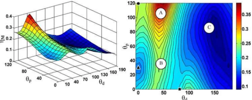
Figure 5 shows manipulator workspace changes based on distinctive parameters variation. By examining this diagram, it is observed that maximum workspace volume occurs in parameters zones which are signed by A and C letters that Hexa manipulator parameters is also there. For example, if a manipulator is asked in proper workspace P 0, revolute joint angle qd is considered between
25 and 40. Of course, if revolute vector angle qd in area A shows arms conditions to manipulator
outside, corresponding point in area C has 180 degree difference from condition A and shows sym-metrical condition inside manipulator. Moreover, it is seen that in P 120, that structural parame-ters of Hunt type manipulator is there, Workspace for all joint axis angles is small and has the min-imum workspace in area B and manipulator will have the minmin-imum workspace by selecting parame-ters of this area.
In order to explore effect of parameters on local kinematic dexterity, it is assumed that the mo-bile platform is in a certain condition [ , , ]=[0, 0, 0.35]x y z . LCI changes diagram is determined based on structural parameters in Figure 6. By observing this diagram, it is concluded that in parameters range that indicate by A, LCI value approaches to zero, it means, by selecting structural parame-ters in this interval, condition of the manipulator approaches to singular condition. By more precise investigations, it is observed that by selecting parameters in this area, rod, arm, and axis of revolute joint are all in a plane that it is called serial singular condition Bonev(2002). For example. If
0
d
q = and P 20are considered, manipulator will be in singular condition in this situation. As it is observed in Figure 6, among three Hexa, Hunt type, and Zamanov type manipulators, Hexa is closer to the singular area rather and the corresponding LCI value is 0.0278. By considering LCI of Zamanov type manipulator in area B (0.1331) and Hunt type manipulator (0.1067) in area C, it is observed that manipulator with selected parameters in these two ranges have proper local dexterity.
Figure 6: Effect of structural parameters variation on local conditioning index.
However, for better comparison of various structures, it is good to use global index of dexterity which shows dexterity distribution all over the workspace. Therefore, in Figure 7, GCI changes are brought based on structural parameters changes.
By examining diagram, it is observed that changes process of homogeneous GCI is relatively similar to local homogenous LCI. A is a parameters area which is generally too near to singular condition that Hexa manipulator is near to this area and does not have proper condition according to condition number. Manipulators located in B and C zones according to their parameters, which are close to Zamanov and Hunt type manipulators, have the best GCI values. In this diagram, the best GCI is correspond to a manipulator with d 48 and with GCI of 0.078.
Effect of structural parameters change on local dynamic conditioning index in certain condition of mobile platform is shown in Figure 8. Checking this Figures shows that the best values are in parameters range indicate by A. in other words, manipulator has more ability to increase accelera-tion in all direcaccelera-tions by selecting structure parameters in this range. It is clear that, Hunt type ma-nipulator is near to this area. Also in zone B that parameters of Hexa and Zamanov type manipula-tor are located, dynamic dexterity is better than manipulamanipula-tors parameters located in zone C.
Figure 8: Effect of structural parameters variation on local dynamic conditioning index.
Figure 9: Effect of structural parameters variation on global dynamic conditioning index.
values will have the best dynamic performance condition by selecting parameters in this area and C is the worst area for GDCI; in other words, it is observed that in cases that revolute vector angles are in a way manipulator arms are toward inside manipulator, manipulator won’t have proper dy-namic condition that cause manipulators arms parallel toward outside to have better dydy-namic dex-terity values comparing when these arms are toward inside manipulators
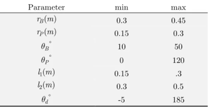
Optimum values of structural parameters are obtained by the modified multi-objective Bees al-gorithm for dynamic and kinematic objective-functions in a prescribed cubic workspace. All geomet-rical and structural parameters in vector γ were considered as designing parameters in simultane-ous dynamic and kinematic indices optimization problem. In addition, mentioned constraints in relations (66) to (70) were considered in optimization. Range of design parameters are presented in Table 4. Pre-determined workspace is considered as a cube by 0.1m width and 0.1m height from z=0.3m to z=0.4m, platform direction is fixed all over platform as x y z 0. Applied param-eters of the modified multi-objective Bees Algorithm are presented in Table 5.
max min
Parameter
0.45 0.3
( )
B
r m
0.3 0.15
( )
P
r m
50 10
B
q
120 0
P
q
.3 0.15
1( ) l m
0.5 0.3
2( ) l m
185 -5
d
q
Table 4: Range of design parameters.
max Parameter
150 n
50 m
20 nsp
.02 ngh (for length type parameters)
2 ngh (for angle type parameters)
Table 5: Parameters of the multi objective Bees Algorithm.
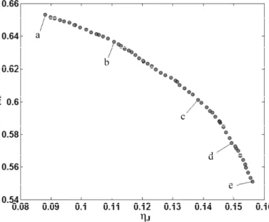
Pareto front diagram related to manipulator obtained by the modified multi-objective Bees Al-gorithm is shown in Figure 10. By checking non-dominate solutions, it is concluded that number of solutions are obtained with proper distribution by this method. Specifications of some points in Pareto front are shown in Table 6. Since it covers all pre-determined solution of workspace, appro-priate to importance of each dynamic and kinematic criteria, one group of existed parameters in Pareto diagram can be selected as manipulator designing parameter. Solutions in Pareto front are compatible with proper ranges obtained from Figures 5 to 9.
with corresponding parameters of point "c" in the middle of Pareto front. by examining the distri-bution of performance indices, it is observed the best values of LCI and LDCI are located in center of each plain. Also, lower plains have better performance index values.
Figure 10: Obtained Pareto-front using modified multi-objective Bees algorithm.
d
q
2( ) l m 1( )
l m
P
q
B
q
( )
P
r m
( )
B
r m
hM
hJ
17.05 0.426
0.172 117.53
39.59 0.193
0.449 0.653
0.087 a
-3.53 0.432
0.173 115.73
13.91 0.210
0.41 0.637
0.109 b
133.27 0.493
0.174 117.13
10.43 0.233
0.439 0.602
0.137 c
125.36 0.498
0.175 116.49
12.01 0.243
0.445 0.574
0.149 d
122.71 0.499
0.171 119.86
10.12 0.249
0.437 0.551
0.156 e
Table 6: Parameters of selected points of Pareto front.
z=0.4 z=0.3
z=0.35
z=0.4
z=0.35 z=0.3
x y
x y
1/
kM
1/
kJ
8 CONCLUSION
In the present study, three well-known manipulators were classified after determining the axis angle of revolute joint and the spherical joint placement on the mobile platform as the distinctive param-eters of 6-RUS parallel manipulators structure. In addition, the effects of these paramparam-eters were investigated on performance criteria including workspace and dynamic and kinematic dexterity. Finally, considering all structural and geometrical parameters and determining proper constraints, optimization problem of the 6-RUS manipulator structure was solved using the modified multi-objective Bees Algorithm. Results of this research show that:
1.There is a specific range of parameters that manipulator workspace gets its maximum value. This range is close to the condition which both adjacent chains are parallel that Hexa manip-ulator is close to such condition. Selecting specified manipmanip-ulator in this area is proper for moving objects in big spaces.
2.By checking local and global dexterity indices values variation, it is seen that areas which rod, revolute vector, and arm are in the same plain, manipulator approaches to singular areas and selecting structure in this area decreases locating precision of manipulators that Hexa manipulator is close to this area.
3.By investigating dynamic dexterity, It is observed; although, local values of indices are good in some configuration, generally base on global dynamic dexterity index, when manipulator arms are aligned toward outside, manipulator is in more proper condition than the time ma-nipulator arms are toward inside.
4.It is observed by comparing three 6-RUS manipulators that Hexa manipulator has more workspace but has less proper kinematic dexterity condition than other manipulators and less locating precision condition. Moreover, there is no proper dynamic condition so this manipu-lator has a proper selection for transferring objects with high acceleration in wide workspace. Although, Hunt type manipulator has limited space, it has proper condition according to condition number that increases its locating precision and has similar dynamic and kinematic conditions to other manipulators. Zamanov type manipulator is in middle of two other ma-nipulators and the only point about this manipulator is that workspace of this manipulator has asymmetrical distribution toward manipulator spherical joints. Due to high symmetry of Hexa and Hunt type workspace than Zamanov type workspace, percentage of inscribed cubic workspace to reachable workspace for Hexa, Hunt are more than Zamanov type.
5.In addition, it is observed that the modified multi-objective Bees Algorithm method is able to find optimum solutions of 6-RUS manipulator multi-objective structure designing. Pareto so-lutions are compatible with mentioned conclusions.
References
Aginaga, J., Zabalza, I., Altuzarra, O., jera, J., (2012). Improving static stiffness of the 6-RUS parallel manipulator using inverse singularities. Robotics and Computer-Integrated Manufacturing 28: 451-479.
Alam, M. N., Akhlaq, A., (2015). Dynamic analysis and vibration control of a multi-body system using MSC Adams. Latin American Journal of Solids and Structures 12(8): 1505-1524.
Asada, H., (1984). Dynamic analysis and design of robot manipulators using inertia ellipsoids. Proceedings of the IEEE International Conference on Robotics and Automation, Atlanta, USA, 13-15 March1984, pp. 94-102. Bonev, I. A. (2002). Geometric analysis of parallel mechanisms, PhD Thesis, Laval University, Quebec, canada. Campos, A., Faveri, G. d., Neto, C. S. F., Reis, A., Garcia, A., (2013). Invers kinematics for general 6-RUS parallel robots applied on UDESC-CEART flight simulatore. 22nd International Congress of Mechanical Engineering (COBEM 2013), Ribeirão Preto, SP, Brazil, 9.
Caro, S., Chablat, D., Lemoine, P., Wenger, P., (2015). Kinematic analysis and trajectory planing of the Or-toglide 5-axis. Proceedings of the ASME International Design Engineering Technical Conferences & Computers and Information in Engineering Conference IDETC/CIE 2015, Boston, USA.
Chablat, D., and Wenger, P., (2003). Architecture Optimization of a 3-DOF Translational Parallel Mechanism for Machining Applications, the Orthoglide. IEEE Transactions on Robotics and Automation 19(3): 403-410.
Clavel, R., (1988). Delta, a fast robot with parallel geometry. Proc 18th Int Symp on Industrial Robots, Lausanne, 91-100.
Clavel, R., (1991). Conception d'un robot parallèle rapide à 4 degrés de liberté, PhD Thesis, EPFL, Lausanne, Switzerland.
Cui, G., Zhang, H., Xu, F., Sun, C., (2014). Kinematics Dexterity Analysis and Optimization of 4-UPS-UPU Parallel Robot Manipulator, Intelligent Robotics and Applications (Springer), 1-11.
Dehghani, M., Ahmadi, M., Khayatian, A., Eghtesad, M., Yazdi, M., (2014). Vision-based calibration of a Hexa parallel robot. Industrial Robot: An International Journal 41: 296-310.
Fassi, I., Legnani, G., Tosi, D., (2005). Geometrical conditions for the design of partial or full isotropic hexapods. Journal of Robotic Systems 22(10): 507-518.
Gil, J., Zabalza, I., Ros, J., Pintor, J., Jiménez, J., (2004). Kinematics and Dynamics of a 6-RUS Hunt-Type Parallel Manipulator by Using Natural Coordinates, On Advances in Robot Kinematics (Springer), 329-335.
Gosselin, C. M., Wang, J., (2000). Static balancing of spatial six degree of freedom parallel mechanisms with revolute actuators. Journal of Robotic Systems 17(3): 159-170.
Gosselin, C. M., Tale Masouleh, M., Duchaine, V., Richard P.-L., imon Foucault, S., Kong, X., (2007). Parallel Mechanisms of the Multipteron Family: Kinematic Architectures and Benchmarking. IEEE International Confer-ence on Robotics and Automation, Roma, Italy, 550-560.
Hesselbach, J., Bier, C., Campos, A., Löwe, H., (2005). Direct kinematic singularity detection of a hexa parallel robot. Proceedings of the IEEE International Conference on Robotics and Automation, Barcelona, Spain, 3238-3243.
Hosseini, M. A., Mohammadi DanialiH.-R., (2011). Dexterous Workspace Shape and Size Optimization of Tricept Parallel Manipulator.International Journal of Robotics 2 (1): 18-25.
Hunt, K., (1983). Structural kinematics of in-parallel-actuated robot-arms. Journal of mechanisms, transmissions and automation in design 105 (4): 705-712.
Khan, W. A., Angeles, J., (2006). The Kinetostatic Optimization of Robotic Manipulators: The Inverse and the Direct Problems. Journal of Mechanical Design 128: 168–178.
Kucuk, s., Bingul, z., (2006). Comparative study of performance indices for fundamental robot manipulators. Robotics and Autonomous Systems 54: 567-573.
Liu, X. J., Wang, J., Gao, F., Wang, L. P., (2002). Mechanism design of a simplified 6-DOF 6-RUS parallel manipulator. Robotica 20(1): 81-91.
Merlet, J. P. (2006). Parallel robots ,Springer.
Nguyen, A. V., Bouzgarrou, B. C., Charlet, K., Béakou, A., (2015). Static and dynamic characterization of the 6-Dofs parallel robot 3CRS. Mechanism and machine theory 93: 65-82.
Pham, D. T., Ghanbarzadeh, A., (2007).Multi-Objective Optimisation using the Bees Algorithm.3rd International Virtual Conference on Intelligent Production Machines and Systems (IPROMS 2007), Whittles, Dunbeath, Scotland, 6.
Pham, D. T., Ghanbarzadeh, A., Koc, E., Otri, S., Rahim, S., Zaidi, M., (2006).The Bees Algorithm a Novel Tool for Complex Optimisation Problems. Proceedings of the 2nd International Virtual Conference on Intelligent Production Machines and Systems, Oxford, United Kingdom, 6.
Pierrot, F., (1990). A new design of a 6-DOF parallel robot. J. of Robotics and Mechatronics 2(4): 308-315.
Rezaei, A., Akbarzadeh, A., (2015). Study on Jacobian, singularity and kinematics sensitivity of the FUM 3-PSP parallel manipulator. Mechanism and machine theory 86: 211-234.
Rezaei, A., Akbarzadeh, A., Nia, P. M., Akbarzadeh-T, M. R., (2013). Position, Jacobian and workspace analysis of a 3-PSP spatial parallel manipulator. Robotics and Computer-Integrated Manufacturing 29 (4): 158-173.
Takeda, Y., Funabashi, H., Ichimaru, H., (1997). Development of spatial in-parallel actuated manipulators with six degrees of freedom with high motion transmissibility. JSME international journal. Series C, dynamics, control, robotics, design and manufacturing 40 (2): 299-308.
Uchiyama, M. A., (1993). 6 dof parallel robot HEXA. Adv Robotics 8: 601- 601.
Wang, F., Chen, Q., Li, Q., (2015). Optimal Design of a 2-UPR-RPU Parallel Manipulator. Journal of Mechanical Design 137(5): 054501.
Wang, L., Zhang, B., Wu, J., (2015). Optimum design of a 4-PSS-PU redundant parallel manipulator based on kinematics and dynamics. Proceedings of the Institution of Mechanical Engineers, Part C: Journal of Mechanical Engineering Science: 1-12.
Wu, J., Wang, J., Li, T., Wang, L., Guan, L., (2008). Dynamic dexterity of a planar 2DOF parallel manipulator in a hybrid machine tool. Robotica 26: 93-98.
Yoshikawa, T., (1985). Dynami Manipulability Of Robot Manipulators. Journal of robotic systems: 113-124.