Comparative Study Of Artificial Neural Network And Box-Jenkins Arima For Stock Price Indexes

Texto

(1)Instituto Superior de Ciências do Trabalho e da Empresa. C O M P A R A T IV E ST U D Y O F A R T IFIC IA L N E U R A L N E T W O R K A N D B O X -JE N K IN S A R IM A FO R ST O C K P R IC E IN D E X E S. Ângela Marisa Roldão Cancela. Dissertation submitted in fulfilment of the requirements for the degree of Master in Data Analysis Prospecting. Advisor:. Prof. Dr. Diana Mendes, assistant professor, ISCTE Business School, Department of Quantitative Methods. September, 2008.

(2) Comparative study of ANN and Box-Jenkins ARIMA for Stock price indexes. Abstract:. The accuracy in forecasting financial time series, such as stock price indexes, has focused a great deal of attention nowadays. Conventionally, the Box-Jenkins autoregressive integrated moving average (ARIMA) models have been one of the most widely used linear models in time series forecasting. Recent research suggests that artificial neural networks (ANN) can be a promising alternative to the traditional ARIMA structure in forecasting. This thesis aims to study the efficiency of ARIMA and ANN models for forecasting the value of four Stock Price Indexes, of four different countries (Germany, Italy, Greece and Portugal), during 2006 – 2007, using the data from preceding 15 years. In order to reach the goal of this study, it is used the Eviews software that allows to find an appropriate ARIMA specification, offered also a powerful evaluation, testing and forecasting tools. In order to predict the time series is used the Matlab software, which provides a package that allows generating a suitable ANN model. It is found that ANN provides forecasted results closest to the actual ones when used the logarithmic transformation. The first difference transformation is required in ARIMA but no one founding model is satisfactory. When this transformation is also used with ANN, the forecasted results are less satisfactory. In fact, it wasn’t possible to compare the efficiency of ARIMA and ANN models for forecasting the time series, due to the founding ARIMA models were not satisfactory. A possible solution would be to reduced the input period of 15 years. Keywords: ARIMA models; Artificial Neural Networks; Backpropagation Algorithm, Stock price index forecasting; Classifications from JEL Classification System: Time-Series Models (JEL:C22); Forecasting and Simulation (JEL:E17).. 2.

(3) Comparative study of ANN and Box-Jenkins ARIMA for Stock price indexes. Resumo:. Actualmente a precisão na previsão de séries financeiras, tais como Índices Accionistas, têm captado uma enorme atenção. Tradicionalmente, o modelo Box-Jenkins Autorregressivos Integrados de Médias Móveis (ARIMA) é um dos modelos lineares mais utilizados na previsão de séries temporais. Pesquisas recentes têm demonstrado que as Redes Neuronais Artificiais (RNA) podem constituir uma potencial alternativa à tradicional estrutura ARIMA, na previsão. Esta tese tem por objectivo o estudo da eficiência dos ARIMA e dos modelos de RNA na previsão de quarto índices accionistas de quatro diferentes países (Alemanha, Itália, Grécia e Portugal), desde 2006 a 2007, considerando os 15 anos antecedentes. De modo a atingir este objectivo, foram utilizados dois softwares. Para determinar uma especificação apropriada para os modelos ARIMA foi utilizado o software Eviews que dispõe, também, de ferramentas poderosas para avaliar e testar os modelos, possibilitando ainda a previsão através dos mesmos. De forma a encontrar modelos RNA apropriados, para prever as séries em estudo, foi utilizado o software Matlab. As RNA forneceram uma boa precisão na previsão das quatro séries logaritmizadas. Uma vez que os modelos ARIMA requerem estacionaridade das séries, foram utilizadas as séries das primeiras diferenças, no entanto não foi encontrado nenhum modelo que pudesse fornecer uma previsão aceitável. Considerando as séries temporais diferenciadas nas RNA, os resultados da previsão foram menos satisfatórios. De facto, não foi possível comparar a eficiência dos modelos na previsão dos índices, uma vez que os modelos ARIMA encontrados não foram satisfatórios. Uma hipótese, na tentativa de encontrar modelos satisfatórios seria reduzir o intervalo de 15 anos de input. Palavras-chave: Modelos ARIMA; Redes Neuronais Artificiais; Algoritmo Backpropagation, Previsão de Índices Accionistas; Classificações do JEL Classification System: Time-Series Models (JEL:C22); Forecasting and Simulation (JEL:E17). 3.

(4) Comparative study of ANN and Box-Jenkins ARIMA for Stock price indexes. Sumário. A previsão é uma ferramenta preciosa na definição de estratégia nos mercados financeiros e, por consequência, na previsão de índices accionistas. Uma boa previsão permite a tomada de decisões mais ponderadas e justificadas, possibilitando que o investidor individual possa actuar sobre este tipo de mercados. Para o investidor colectivo a utilização desta ferramenta é ainda mais notável, uma vez que, em muitos casos, para além da gestão do próprio capital, permite também garantir as responsabilidades assumidas perante o cliente, como acontece no caso das seguradoras e bancos. No entanto, dada a complexidade de alguns processos que intervêm nas estratégias definidas, tal como a inflação, é difícil fazer previsão em tempo real. Por esta razão, são, muitas vezes, utilizados modelos lineares. O modelo Box-Jenkins Autorregressivos Integrados de Médias Móveis (ARIMA) é um dos modelos lineares mais utilizados na previsão de séries temporais, existindo vários artigos sobre a previsão através desses mesmos modelos. Contudo, pesquisas recentes, têm mostrado uma boa performance na previsão através das Redes Neuronais Artificiais (RNA). Com o intuito de comparar a performance na previsão de índices accionistas, através destes dois modelos, foram utilizados quatro índices accionistas, de quatro diferentes países – Portugal, Grécia, Alemanha e Itália, integrando estes dois últimos o G8. Para tal, considerouse um histórico de 15 anos a fim de prever o valor dos índices entre 2006 e 2007. Para determinar uma especificação apropriada para os modelos ARIMA foi utilizado o software Eviews que dispõe, também, de ferramentas poderosas para avaliar e testar os modelos, possibilitando ainda a previsão através dos mesmos. De forma a encontrar modelos RNA apropriados, para prever as séries em estudo, foi utilizado o software Matlab. Os resultados obtidos através dos dois modelos foram muito similares, quando aplicados aos diferentes índices. Verificou-se uma boa performance na previsão dos quatro índices entre. 4.

(5) Comparative study of ANN and Box-Jenkins ARIMA for Stock price indexes. 2006 e 2007, utilizando os modelos RNA. Todavia, não foi possível comparar os modelos, uma vez que os modelos ARIMA encontrados, não foram satisfatórios. A estacionaridade das séries é requerida pelos ARIMA, no entanto, no período considerado como input, nenhuma das séries era estacionária, pelo que se utilizaram as séries das primeiras diferenças. Apesar da diferenciação, não foi possível obter resultados satisfatórios com os modelos ARIMA encontrados. Resultados similares a estes foram obtidos nas RNA, quando consideradas como input cada uma das quatro séries diferenciadas. É possível que a existência de perda de informação valiosa, no momento da diferenciação das séries em estudo, torne os modelos ARIMA pouco satisfatórios, uma vez que, quando se consideram as séries originais se obtêm resultados satisfatórios nas RNA. Uma hipótese, na tentativa de encontrar modelos satisfatórios seria reduzir o intervalo de 15 anos de input.. 5.

(6) Comparative study of ANN and Box-Jenkins ARIMA for Stock price indexes. List of figures:. Figure 1.4.1: Summarized proceeding to modulate an ARIMA ................................................ 18 Figure 1.4.2: Feedforward Neural Networks (single hidden layer network) ............................. 21 Figure 1.4.3: Transfer functions ................................................................................................. 24 Figure 2.1: Graphical representation of natural logarithm of the four Stock price index .......... 33 Figure 2.2: The correlogram of LOGBD and the correlogram of LOGGR ............................... 34 Figure 2.3: The correlogram of LOGITL and the correlogram of LOGPT ............................... 34 Figure 2.4: The correlograms of DLOGBD and of DLOGITL .................................................. 38 Figure 2.5: The correlograms of DLOGGR and of DLOGPT ................................................... 38 Figure 2.6: ARIMA(1,1,1) estimation output ............................................................................ 40 Figure 2.7: ARIMA(2,1,2) estimation outputs for DLOGBD .................................................... 41 Figure 2.8: Correlogram of residuals of ARIMA(2,1,2) model with DLOGBD ........................ 42 Figure 2.9: The results of Breusch-Godfrey (LM) test .............................................................. 42 Figure 2.10: Histogram and some statistics of residuals of ARIMA(2,1,2) model with DLOGDB ...................................................................................................................................................... 43 Figure 2.11: estimation output of ARIMA(2,1,0) with DLOGGR ............................................. 44 Figure 2.12: ARIMA(1,1,2) estimation output with DLOGITL ................................................ 45 Figure 2.13: ARIMA(1,1,2) estimation output with DLOGPT .................................................. 47 Figure 2.14: Forecasting outputs of LOGBD trough ANN – in Matlab .................................... 52 Figure 2.15: Forecasting outputs of DLOGBD trough ANN – in Matlab ................................. 53 Figure 2.16: Forecasting outputs of LOGGR trough ANN – in Matlab .................................... 54 Figure 2.17: Forecasting outputs of DLOGGR trough ANN – in Matlab ................................. 55 Figure 2.18: Forecasting outputs of LOGITL trough ANN – in Matlab ................................... 56 Figure 2.19: Forecasting outputs of DLOGITL trough ANN – in Matlab ................................ 57 Figure 2.20: Forecasting outputs of LOGPT trough ANN – in Matlab ..................................... 58 Figure 2.21: Forecasting outputs of DLOGPT trough ANN – in Matlab .................................. 59. I.

(7) Comparative study of ANN and Box-Jenkins ARIMA for Stock price indexes. List of tables:. Table 2.1: Descriptive statistics .................................................................................................. 31 Table 2.2: The resume of Eviews results for the Unit Root Test ................................................ 37 Table 2.3: The Eviews values for the Information criteria for ARIMA(p,1,q) for DLOGBD ... 40 Table 2.4: The Eviews values for the Information criteria for ARIMA(p,1,q) for DLOGGR ... 44 Table 2.5: The Eviews values for the Information criteria for ARIMA(p,1,q) for DLOGITL .. 45 Table 2.6: The Eviews values for the Information criteria for ARIMA(p,1,q) for DLOGPT .... . 46 Table 2.7: Forecasting results of ANN model for LOGBD time series ..................................... 51 Table 2.8: Forecasting results of ANN model for DLOGBD time series .................................. 52 Table 2.9: Forecasting results of ANN model for LOGGR time series ..................................... 53 Table 2.10: Forecasting results of ANN model for DLOGGR time series ................................ 54 Table 2.11: Forecasting results of ANN model for LOGITL time series .................................. 55 Table 2.12: Forecasting results of ANN model for DLOGITL time series ................................ 56 Table 2.13: Forecasting results of ANN model for LOGPT time series .................................... 57 Table 2.14: Forecasting results of ANN model for DLOGPT time series ................................. 58 Table 3.1: The minimum and the maximum value of the RMSE, considering all forty-two networks with the logaritmized time series ................................................................................. 62 Table 3.2: The minimum and the maximum value of the RMSE, considering all forty-two networks with the first differences logaritmized time series ....................................................... 63. II.

(8) Comparative study of ANN and Box-Jenkins ARIMA for Stock price indexes. Contents:. INTRODUCTION.................................................................................................................... 1 Chapter 1 1 – LITERATURE REVIEW.............................................................................................. 4 1.1 – ARIMA MODELS ........................................................................................................ 4 1.1.1 – ARIMA models – Univariate ................................................................................. 5 1.1.2 – ARIMA models – Multivariate .............................................................................. 6 1.2 – NEURAL NETWORKS MODELS .............................................................................. 7 1.3 – PROPERTIES OF FINANCIAL TIME SERIES.......................................................... 8 1.4 – MODELS USED ......................................................................................................... 10 1.4.1 – Classical methods for time series forecasting ...................................................... 11 1.4.2 – Artificial Neural Networks for time series forecasting ........................................ 20 1.4.2.1 – Multi-layer Feedforward Neural Networks....................................................... 20 1.4.2.2 – Transfer Function in ANN ................................................................................ 23 1.4.2.3 – Learning Rule.................................................................................................... 25 1.4.2.4 – Backpropagation learning algorithm................................................................. 25 1.4.2.4.1 – Stochastic gradient descent backpropagation learning algorithm .................. 26 Chapter 2 2 – INPUT DATA, MODELS SELECTION AND RESULTS....................................... 30 2.1 – DATA AND SOME DESCRIPTIVE STATISTICS .................................................. 30 2.2 – THE ARIMA(p,d,q) MODEL SELECTION .............................................................. 38 2.2.1 –ARIMA(p,1,q) model selection for the Stock price index of Germany................ 38 2.2.2 –ARIMA(p,1,q) model selection for the Stock price index of Greece ................... 43 2.2.3 –ARIMA(p,1,q) model selection for the Stock price index of Italy ....................... 44 2.2.4 – ARIMA(p,1,q) model selection for the Stock price index of Portugal ................ 45 2.3 – THE ANN MODEL SELECTION ............................................................................. 46 2.3.1 – Feedforward backpropagation network for the stock price index of Germany.... 49 2.3.2 – Feedforward backpropagation network for the Stock price index of Greece ...... 52 2.3.3 – Feedforward backpropagation network for the Stock price index of Italy .......... 54 2.3.4 – Feedforward backpropagation network for the Stock price index of Portugal .... 56 Chapter 3 3 – DISCUSSIONS AND CONCLUSIONS ..................................................................... 59 3.1 – THE ARIMA RESULTS ............................................................................................ 59 3.2 – THE ANN RESULTS ................................................................................................. 60 3.3 – ARIMA VERSUS ANN AND FUTURE WORKS ..................................................... 63 References ............................................................................................................................... 65 . III.

(9) Comparative study of ANN and Box-Jenkins ARIMA for Stock price indexes. INTRODUCTION. Forecasting future events based on knowledge given in current data has fascinated people throughout history and, consequently, several techniques have been developed to face this problem of predicting the future behaviour of a particular series of events. Forecasting is a key activity for strategy makers. Given the complexity of the fundamental processes strategy objectives, such as inflation, stock market returns or stock indices, and the difficulty of forecasting in real-time, choice is often taken to simple models. The most well known and widely used methods are based on linear probabilistic models using the autoregressive (AR), the moving average (MA), the autoregressive/moving average (ARMA) and the integrated ARMA models for nonstationary time series. These models are usually estimated either by least squares or maximum likelihood method. They are quite popular since the procedure involved are easy to understand, and the results are also easy to interpret. However, ordinary least squares methodology is employed to obtain parameters in a simple linear model only. This technique becomes irrelevant when dealing with a complex or a nonlinear model. Besides, strict assumptions concerning the specification of the model and the estimation of parameters have to be satisfied to this method to produce meaningful results. Recent studies showed that a considerable number of economic relationships are either nonlinear in the parameters or even chaotic. Of course, linear regression analysis cannot be applied with success in these cases. Nonlinear least squares methods seem to be the most used in order to obtain the parameters in nonlinear models. However, one cannot derive a standard formula for parameters in these models. The computational procedures are fairly complex even though it is based on the same principles as in the ordinary least squares.. 1.

(10) Comparative study of ANN and Box-Jenkins ARIMA for Stock price indexes. In last few years some other techniques, such as genetic algorithms and neural networks, have been introduced. They have the ability to approximate nonlinear functions, and parameters are updated adaptively. The interest in Artificial Neural Networks has increased tremendously lately. Artificial Neural Networks models are applied in many different scientific fields because of their storage and learning capabilities. They provide new ways to solve difficult problems and they are extremely successful in real life situations. There are five main areas in which Artificial Neural Networks models are used: control system, facial and handwriting recognition, medical diagnosis, classification and forecasting. Trading in stock market indices has gained an extraordinary popularity in major financial markets around the world. The increasing diversity of financial index related instruments, along with the economic growth enjoyed in last few years, has expanded the dimension of global investment opportunity either for individual investors or institutional investors. These index vehicles provide effective means for investors to hedge against potential market risks. They, also, create new profit making opportunities for market speculators and arbitrageurs. Thus, being able to accurately forecast a stock market index has profound implications and significance to researches and practitioners. Therefore we can imagine forecasting as an enormous relevance when we are talking about predict the direction/sign of stock index movement.. In recent years, there has been a growing number of studies looking at the direction or trend of movements of various kinds of financial instruments. Such as Maberly (1986) that explores the relationship between the direction of intraday price change; Wu and Zhang (1997) investigate the predictability of the direction of change in future spot exchange rate; 0’Conner, et al. (1997) conduct a laboratory-based experiment and conclude that individuals show different tendencies and behaviours for upward and downward series. This further demonstrates the usefulness of forecasting the direction of change in price level, that is, the importance of being able to classify the future return as gain or a loss. There are also some studies providing a comparative evaluation of different classification techniques regarding their ability to predict the sign of the index return Such as Leung M., et 2.

(11) Comparative study of ANN and Box-Jenkins ARIMA for Stock price indexes. al. (2000) whom evaluate the efficacy of several multivariate classification techniques relative to a group of level estimations approaches. They also conduct time series comparisons between the two types of models on the basis of forecast performance and investment return.. The aim of this study is to evaluate the performance of a classical (ARIMA) and an artificial intelligence (ANN) forecasting techniques for four financial time series of four different countries. The studied stock price indexes, belongs to four different countries, Germany and Italy, which are part of the G8 group and Portugal and Greece. Theoretically, both techniques are very similar in that they attempt to discover the appropriate internal representation of the time series data. In order to reach the goal of this study two softwares will be used. The Eviews software will able to find an appropriated ARIMA model in order to predict each one of the four time series, while Matlab software will allow to generate the ANN model to each one of the same time series.. This thesis is divided into three Chapters. An overview of the essential features and some technical characteristics of the proposed methodologies are firstly approach on Chapter 1, mentioning its applicability to similar data. An extensive description of how to find an adequate ARIMA model is also done in this chapter. Similarly is discussed basic theory underlying the construction of Neural Networks architecture and shown how to approximate the system with backpropagation technique. Chapter 2 is divided in three parts. On the first one is done a brief description of the data as well as show some descriptive statistics. The second and the third parts are divided into four sections, doing the selection of an ARIMA and an ANN model, respectively, for each stock price index. In Chapter 3 are discussed the results obtained in Chapter 2, as well as, it is conclude about this thesis with a perspective on what has been achieved and identifies some prospective topics for further research. 3.

(12) Comparative study of ANN and Box-Jenkins ARIMA for Stock price indexes. Chapter 1. 1 – LITERATURE REVIEW. 1.1 – ARIMA MODELS. Early efforts to study time series, particularly in the 19th century, were generally characterized by the idea of a deterministic world. Yule (1927) launched the notion of stochasticity in time series by assuming that every time series can be regarded as the realization of a stochastic process. Based on this simple idea, a number of time series methods have been developed since then. Researchers such as Slutsky (1937), Walker (1931), Yaglom (1955), and Yule (1927) first formulated the concept of autoregressive (AR) and moving average (MA) models. A considerable body of literature has appeared in the area of time series, dealing with parameter estimation, identification, model checking and forecasting. Box and Jenkins had integrated the existing knowledge, in 1970, with the book “Time Series Analysis: Forecasting and Control” which has had an enormous impact on the theory and practice of modern time series analysis and forecasting. They also developed a coherent, versatile three-stage iterative cycle for time series identification, estimation and validation, known as the Box–Jenkins approach. With the introduction of specialized software, it was observed an explosion in the use of autoregressive integrated moving average (ARIMA) models and their extensions in many areas of science. Several papers were written about forecasting discrete time series processes 4.

(13) Comparative study of ANN and Box-Jenkins ARIMA for Stock price indexes. through univariate ARIMA models, transfer function (dynamic regression) models, and multivariate (vector) ARIMA. Often these studies were of empirical nature, using one or more benchmark methods/models as a comparison. They have also been the key to new developments, see for instance Gooijer (2006).. 1.1.1 – ARIMA models – Univariate. Although Box-Jenkins methodology shown that various models could, between them, mimic the behaviour of diverse types of series, there was no algorithm to specify a model uniquely. Therefore many techniques and methods have been suggested in order to increase mathematical rigour to the search process of an ARMA model, including Akaike’s information criterion (AIC), Akaike’s final prediction error (FPE), and the Bayes information criterion (BIC). Often these criteria come down to minimizing (in-sample) one-step-ahead forecast errors, with a penalty term for overfitting. There are some methods for estimating the parameters of an ARMA model such as the least squares estimator. Although these methods are equivalent asymptotically, in the sense that estimates tend to the same normal distribution, there are large differences in finite sample properties, which may influence forecasts. In order to minimize the effect of parameter estimation errors on the probability limits of the forecasts it is recommended the use of full maximum likelihood. More recently, K i m ( 2 0 0 3 ) considered parameter estimation and forecasting of AR models in small samples. He found that (bootstrap) bias-corrected parameter estimators produce more accurate forecasts than the least squares estimator. L a n d s m a n a n d D a m o d a r a n ( 1 9 8 9 ) presented evidence that the James-Stein ARIMA parameter estimator improves forecast accuracy relative to other methods, under Mean Square Error (MSE) loss criterion. If a time series is known to follow a univariate ARIMA model, forecasts using disaggregated 5.

(14) Comparative study of ANN and Box-Jenkins ARIMA for Stock price indexes. observations are, in terms of MSE, at least as good as forecasts using aggregated observations. However, in practical applications, there are other factors to be considered, such as missing values in disaggregated series or outliers when the ARIMA model parameters are estimated. When the model is stationary, Hotta and Cardoso Neto (1993) showed that the loss of efficiency using aggregated data is not large, even if the model is not known. Thus, prediction could be done either by disaggregated or aggregated models. Usual univariate ARIMA modelling has been shown to produce one-step-ahead forecasts as accurate as those produced by competent modellers (Hill and Fildes, 1984; Libert, 1984; Poulos, et al., 1987). Rather than adopting a single AR model for all forecast horizons, Kang (2003) empirically investigated the case of using a multi-step-ahead forecasting AR model selected separately for each horizon. The forecasting performance of the multi-step-ahead procedure appears to depend on, among other things, optimal order selection criteria, forecast periods, forecast horizons, and the time series to be forecast.. 1.1.2 – ARIMA models – Multivariate. A multivariate generalization of the univariate ARIMA model is the vector ARIMA (VARIMA) model. The population characteristics of VARMA processes appear to have been first derived by Quenouille (1957). VARIMA models can accommodate assumptions on exogeneity and on contemporaneous relationships, they offered new challenges to forecasters and policymakers. Vector autoregressions (VARs) constitute a special case of the more general class of VARMA models. In essence, a VAR model is a fairly unrestricted (flexible) approximation to the reduced form of a wide variety of dynamic econometric models. VAR models can be specified in a number of ways. In general, VAR models tend to suffer from “overfitting” with too many free insignificant parameters. As a result, these models can provide poor out of sample forecasts, even though within-sample fitting is good; see, e.g., Liu, et al. (1994) and Simkins (1995). Instead of restricting some of the parameters in the usual way, Litterman 6.

(15) Comparative study of ANN and Box-Jenkins ARIMA for Stock price indexes. (1986) and others imposed a prior distribution on the parameters, expressing the belief that many economic variables behave like a random walk. The Engle and Granger (1987) concept of cointegration has raised various interesting questions regarding the forecasting ability of error correction models (ECMs) over unrestricted VARs.. 1.2 – NEURAL NETWORKS MODELS. The exceptional characteristic of the human brain it is the ability to learn from the past, which is facilitated by the complex system of sending and receiving electrical impulses among neurons. These facts has fascinated numerous researchers and led to the creation of a cognitive science, also known as artificial intelligence. The construction of a network, known as an artificial neural network (ANN) simulates brain characteristics. Neural derives from neuron, and artificial from the fact that it is not biological. Unlike the brain, the ANN performs discrete operations, which are made possible with electronic computers’ ability to swiftly perform complex operations. In 1943, McCulloch and Pitts developed the first computing machines that intend to simulate the structure of the biological nervous system and could perform logic functions through learning. The output resulting from this network was a combination of logic functions, which were used to transmit information from one neuron to another. This eventually led to the development of the binary probit model. According to this model, the neural unit could either swhich on or off depending on whether the function was activated or not. A threshold determines the activation of the system: if the input is greater than the threshold, then the neuron is activated and equal to 1, otherwise it is 0. Donald Hebb (1949) introduced the first learning law. This learning law, also known as Hebb learning rule, is based on simultaneous combinations of neurons capable of strengthening the connection between them. The work of McCulloch and Pitts influenced another researchers such as, Rosenblatt (1962), 7.

(16) Comparative study of ANN and Box-Jenkins ARIMA for Stock price indexes. that developed advanced models that had ability to learn, of which the best known is the “perceptron”. It is a single feedforward network. The output obtained from this single layer is the weighted sum of different inputs. A significant advance in Neural Networks came in 1967 with the introduction of the smooth sigmoid function as activation function by Cowan. This function has the ability to approximate any nonlinear function. Instead of switching from off to on like the perceptron, the activation function assists the output function to turn on gradually as it is activated. In 1974, Werbos published the “backpropagation” learning method. The backpropagation technique enables the determination of parameter values for which the error is minimized. Prior to the introduction of back-propagation method, it was difficult to determine multiple parameter values. Since the 1940s, Artificial Neural Network (ANN) have been used in various applications in engineering. As artificial intelligence have improved, they also began to be used in the solution of medical, military and astronomical problems. Recently, ANN have been regularly applied to the research area of finance, such as stock market prediction, and bankruptcy perdition of economic agents. But the largest application of neural network in economics and finance is found in the area of forecasting time series, due to their ability to classify a set of observations into different categories, and their forecasting aptitude.. 1.3 – PROPERTIES OF FINANCIAL TIME SERIES. The predictability of most common financial time series such as stock prices is a controversial issue and has been questioned in scope of the efficient market hypothesis (EMH). The EMH states that the current market price reflects the assimilation of all the information available. This means that given the information, no prediction of future changes in the price can be made. As new information enters the system the unbalanced state is immediately discovered and quickly eliminated by a correct change in market price. In recent years, the EMH became a controversial issue due to many reasons. On one side, it 8.

(17) Comparative study of ANN and Box-Jenkins ARIMA for Stock price indexes. was shown in some studies that excess profits can be achieved using only past price data, on the other side it is very difficult to test the strong form due to lack of data. Another reason that helps the predictability being a complex task are some statistical properties of the time series that are different at different points in time. For example the volatility (standard deviation) is different during different periods. There are periods, where the index values fluctuates greatly on a single day, and more calm periods. And, of course, financial time series are influenced by business cycle.. We can’t forgotten that financial time series are usually very noisy, i.e., there is a large amount of random (unpredictable) day-to-day variations. The events, such as interest rate changes, announcements of macroeconomic news as well as political events are random and unpredictable and contribute to the noise in the time series. The noisy nature of financial time series makes it difficult to distinguish a good prediction algorithm from a bad one. However, forecasting is a key activity to define strategies in various fields, nowadays is crucial when trading in stock market indices. It has broadened the dimension of global investment opportunity to both individual and institutional investors, as provide an effective means for investors to hedge against potential market risks and create new profit making opportunities for market speculators and arbitrageurs. In many forecasting situation, more than one component is needed to capture the dynamics in a series to be forecast. Usually, a time series could be defined as:. y t = Tt + St + Ct + εt. €. (1.3.1). where T is the trend component, S is the seasonal component, C is the cyclical component and. ε. is the residue component, which is white noise. Typically, it is assumed that each. component is uncorrelated with all other components at all leads and lags.. €. 9.

(18) Comparative study of ANN and Box-Jenkins ARIMA for Stock price indexes. 1.4 – MODELS USED. Traditionally, the autoregressive integrated moving average (ARIMA) model has been one of the most widely used models in time series prediction. Recent research activities in forecasting with ANN suggest that ANN can be a promising alternative to the traditional ARIMA structure. These linear models and ANN are often compared with mixed conclusions in terms of the superiority in forecasting performance. The ARIMA time series models allow Yt , random variable, to be explained by past, or lagged values of Y itself and stochastic error terms. € An ANN consists of several layers of nodes: an input layer, an output and zero or more. hidden layers. The input layer consists of one node for each independent variable, while the output layer consists of one or more nodes that correspond to the final decision. The hidden layers lie in between, and each consists of several nodes that receive inputs from nodes in layer below them and feed their outputs to nodes in layers above. There are several papers dealing with the comparison of different forecasting methods. In what follows, it is briefly review some of them. In 2000, Leung et al. evaluated the efficacy of several multivariate classification techniques relative to a group of level estimation approaches, conducted time series comparisons between the two types of models and the basis of forecast performance and investment return. The classification models used, by them, to predict direction/sign of stock index movement based on probability, include linear discriminant analysis, probit, logit and probabilistic neural network. Their empirical experimentation suggests that probabilistic neural network was the best performer among the forecasting models evaluated in their study. Ho et al. (2002), drew a comparative study between ANN and Box-Jenkins ARIMA modelling in time series prediction. The neural network architectures evaluated by them, in this study, were the multiplayer feedforward network and the recurrent neural network 10.

(19) Comparative study of ANN and Box-Jenkins ARIMA for Stock price indexes. (RNN). They concluded that both ARIMA and RNN models outperform the feedforward model; in terms of lower predictive errors and higher percentage of correct reversal detection. They also investigated the effect of varying the damped feedback weights in recurrent net, and they found that RNN at the optimal weighting factors gave more satisfactory performances than ARIMA model. Phua, et al. (2003) applied generically evolved neural networks models to predict the Straits Times Index of the Stock Exchange of Singapore. Their studies show that satisfactory results can be achieved when applying these techniques. Kamruzzaman and Sarker (2003) investigated three ANN based forecasting models to predict six foreign currencies against Australian dollar using historical data and moving average technical indicators, and a comparison was made with traditional ARIMA model. All the ANN based models outperformed ARIMA model measured on five performance metrics used by them. Their results demonstrate that ANN based model can forecast the exchange rates closely.. Following the papers cited above and taking in consideration the growing interest in forecasting, in this study it is expected to evaluate the performance of an ARIMA and an ANN model when applied for predicting four time series representing stock price indexes.. 1.4.1 – Classical methods for time series forecasting. On a classical time series forecasting it is assumed that the future value is a linear combination of historical data. There are several time series forecasting models, however the most highly popularized is Box-Jenkins ARIMA model which was successfully applied in financial time series forecasting, and also as a promising tool for modelling the empirical dependencies between successive time between failures.. 11.

(20) Comparative study of ANN and Box-Jenkins ARIMA for Stock price indexes. Before broaching the structure of the ARIMA model it is done a brief overview of basic concepts of linear time series analysis such as stationarity, seasonality, unit-root nonstationarity and a short reference to the most classical common types of time series forecasting process. A random or stochastic process is a collection of random variables ordered in time. If a random variable, Y, it is continuous will be denote as Y(t), and if it is discrete will be denoted by Yt . A type of stochastic process that received a great deal of attention and scrutiny by time series analysts is the stationary stochastic process. €. Stationarity. Broadly speaking, a time series is said to be stationary if the mean, the variance and the autocovariance (at various lags) remain the same no matter at what point we measure them, that is, they are constant over the time. A time series Yt is said to be strictly stationary if the joint distribution of ( Yt1 , Yt2 , …, Yt ) and k. of ( Yt1 −t , Yt2 −t , …, Ytk −t ) are identical for all t, where k ∈ /N , t i ∈ /N and i = 1,,k , i.e., strict stationary requires that the joint distribution of ( Yt1 , Yt2 , …, Yt ) is€invariant under time shift. € € € k. €. € € € € € This is a very strong condition that is hard to verify empirically. A weaker version of € € € stationarity is often assumed. A time series Yt is weakly stationary if both the mean of Yt and the covariance between Yt and Yt−s are time-invariant, s ∈ /N . Thus Yt is weakly stationary if • •. € €. E(Yt ) = µ , which is a constant and € Cov(y t , y t−s ) = γ s , is called lag-s autocovariance of€Yt . € € €. €. Stationarity is very important in time series because if a time series is nonstationary (time € varying mean or a time-varying variance or both) it’s behaviour only can be study for the period under consideration. Each set of time series data will therefore be a particular episode. Thus, for the purpose of forecasting nonstationary time series may be of little practical value.. Autocorrelation function (ACF). The correlation coefficient between two random variables X and Y, measures the strength of linear dependence between X and Y, and take values 12.

(21) Comparative study of ANN and Box-Jenkins ARIMA for Stock price indexes. between -1 and 1. It is defined as. ρ X ,Y =. Cov(X,Y) = Var(X)Var(Y ). E[(X − X )(Y − Y )] E(X − X ) 2 E(Y − Y ) 2. ,. where X is the mean of X and Y the mean of Y. If ρ X ,Y = 0 , then X and Y are independent random variables. € time series Yt .€When the linear dependence between Yt and it’s € € Consider a weakly stationary past values. Yt−i is of interest, the concept of correlation is generalized to autocorrelation. The. correlation coefficient between Yt and Yt−s is called the lag-s autocorrelation of Yt and is € € commonly denoted by ρ s , which under the weak stationarity assumption is a function defined by€. €. €. € T. ∑ (Y − Y )(Y t. €. ρs =. t−s. t= s+1. −Y ) .. T. ∑ (Y − Y ). 2. t. t=1. As a matter of fact, a linear time series model can be characterized by its Autocorrelation function (ACF), and linear time series modelling makes use of the sample ACF to capture the € linear dynamic of the data. If ρ1 is nonzero, it means that the series is first order serially correlated. If ρs dies off more or less geometrically with increasing lag s, it is a sign that the series obeys a low-order autoregressive process. If ρs drops to zero after a small number of lags, it is a sign that the. €. series obeys a low-order moving-average process.. €. € White noise. A time series Yt is called white noise if Yt is a sequence of independently and identically distributed (iid) random variables with finite mean and variance. In particular, if Yt is normally distributed with mean zero and variance σ 2 and no serial correlation, then it is € € said to be Gaussian white noise. For a white noise series, all the ACFs are zero. In practice, if € all sample ACFs are close to zero, then the series is a white noise series. €. Random walk process. A random walk process is generally an approach used in the equity market to describe, for example, the behaviour of stock prices or exchange rates. This process 13.

(22) Comparative study of ANN and Box-Jenkins ARIMA for Stock price indexes. continually drifts from any expected value in a specific period of time. In this approach it is not considered any constant value or constant variance over time. Usually in the literature we can distinguish between two types of random walk process: random walk without a drift (1.4.1) (i.e., no constant or intercept term) and random walk with a drift (1.4.2) (i.e., a constant term is present):. € € €. y t = y t−1 + εt. (1.4.1). y t = α + y t−1 + εt. (1.4.2). where y 0 is a real number denoting the starting value of the process, and εt is a white noise series and α is known as drift parameter.. € If a trend in a time series process is completely predictable and not variable, it is said a deterministic trend, whereas if it is not predictable, it is said a stochastic trend.. Unit Root Process. Writing a random walk process as (1.4.3). y t = ρ y t−1 + εt , −1 ≤ ρ ≤ 1. €. then if ρ=1, we have a random walk process without a drift. Moreover, if ρ is in fact 1, we face what is known as the unit root problem, that is, a situation of nonstationarity; thus in this case the variance of Yt is nonstationary. The name “unit root” is due the fact that ρ=1. However, if |ρ|<1, then it can be shown that the time series Yt is stationary. In practice, it is € important to find out if a time series process has a unit root or not.. € In the following definitions, the constants will be defined by α i with i ∈ /N or by β i with. i ∈ /N . Autoregressive process. Consider the following equation €. €. €. €. 14.

(23) Comparative study of ANN and Box-Jenkins ARIMA for Stock price indexes. (1.4.4). Yt = α 0 + α1Yt−1 + εt. € €. where εt is white noise, i.e., a random number from a distribution with following properties: •. E(εt ) = 0. •. Var(εt ) = σ 2 and. • Cov(εt−s,εt ) = 0 , if s ≠ 0 € Cov means Covariance and is a measure of association between two variables, that is, €. €. n. Cov(X,Y ) =. €. 1 ∑ (X i − X )(Yi − Y ) n i=1. (1.4.5). Consequently, white noise is a sequence of randomly distributed real numbers with zero mean and no association between numbers drawn at different points of time. As the current value, Yt , is expressed in terms of the past value, Yt−1 , the equation (1.4.4) is called AR(1) model or first order autoregressive model, where it is assumed that Yt−1 and εt are independent. €. €. € € The extension of the equation presented before to two consecutive past values would lead to an AR(2) model, that is 2. Yt = α 0 + α1Yt−1 + α 2Yt−2 + εt = α 0 + ∑α iYt−i +εt. (1.4.6). i=1. €. More generally, we say that a variable Yt is autoregressive of order p, AR(p), with p ∈ /N , if it is a function of its p past values and can be expressed as p. €. €. Yt = α 0 + ∑α pYt− p +εt. (1.4.7). i=1. €. Moving Average process. When the current value, Yt , of a time series is expressed in terms 15. €.

(24) Comparative study of ANN and Box-Jenkins ARIMA for Stock price indexes. of current and previous values of the stochastic error term εt , we are talking about the first order moving average, MA(1), that is. €. Yt = β 0εt + β1εt−1. €. (1.4.8). where εt , is a purely random term with mean zero and variance σ 2 . When (1.4.8) contains the q most recent values of the stochastic error term, we have a MA(q). €. model, which is given by the following equation:. €. q. Yt = β 0εt + β1εt−1 +  + β qεt−q = ∑ β iεt−i. (1.4.9). i= 0. €. Autoregressive Moving Average process. An Autoregressive Moving Average process, ARMA model, is a combination between the autoregressive model and a moving average model. In general, an ARMA (p,q) is a combination of an AR(p), equation (1.4.7), and MA(q), equation (1.4.9), and can be written as p. q. Yt = α 0 + ∑α iYt−i +∑ β iεt−i i=1. €. (1.4.10). i=1. In practice, one applies the ARMA process not to the time series, but to transformed time series. It is often the case, that the time series of differences is stationary in spite of the nonstationarity of the underlying process. Stationary time series can be well estimated by the ARMA model. That leads to the definition of the ARIMA model.. Autoregressive Integrated Moving Average process. Popularly known as the Box-Jenkins methodology, but technically known as the ARIMA methodology, these methods emphasis is not on constructing single or simultaneous equation models, but on analysing the probabilistic, or stochastic, properties of economic time series on their own under the philosophy “let the data speak for themselves”. Unlike the regression models, in which Yt is explained by n regressor X1 , X 2 , …, X n , the ARIMA time series models allow Yt to be € €. €. €. €. 16.

(25) Comparative study of ANN and Box-Jenkins ARIMA for Stock price indexes. explained by past, or lagged values of Y itself and stochastic error terms. For these reason, these models are sometimes called theoretic models because they are not derived from any economic theory – and economic € theories are often basis of simultaneous equation models. The previous mentioned models are based on assumptions that the time series involved are (weakly) stationary. But it is known that many economic time series are nonstationary, that is, they are integrated. If a time series is integrated of order 1, i.e., I(1), it’s first differences are I(0), that is, stationary. Similarly, if a time series is I(2), it’s second difference is I(0). In general, if a time series is I(d), after differencing it d times we obtain an I(0) series. Therefore if we needed to difference a time series d times in order to make it stationary and then apply the ARMA(p,q) process to it, we say that the original time series is an ARIMA(p,d,q) process, that is, it is an autoregressive integrated moving average time series. The first task in estimating ARIMA model is to specify p (the number of autoregressive terms), d (the number of first differences or other transformation) and q (the number of moving-average terms). Once these parameters have been chosen, the job of specifying the ARIMA equation is complete, and the computer estimation package will then calculate estimates of the appropriate coefficients. Because the error term in the moving average process is, of course, not observable, a non linear estimation technique must be used instead of OLS. For the forecasting purposes the usage of ARIMA model can be summarized by the flowchart shown in the following figure.. 17.

(26) Comparative study of ANN and Box-Jenkins ARIMA for Stock price indexes. Figure 1.4.1: Summarized proceeding to modulate an ARIMA. In the first step, the differencing operator is applied to the time series until it becomes stationary. The determination whether Yt is stationary or not can be performed by visualizing the correlogram of Yt . It’s rare to find in economic examples a situation calling for d > 1. If the ACF of the dependent variable approaches zero as the number of lags increases (“the € correlogram converges to zero”), then the series is stationary; a nonstationary series will show € little tendency for the ACFs to decrease in size as the number of lags increase. After an examination of the plot and the ACF makes the researcher feel comfortable that enough transformations have been applied to make the resulting series stationary. The next step is to choose integer values for p and q. After the d value is determined, any non-zero mean is removed from the time series (the mean is calculated and subtracted from each element of the time series). Next, the parameters p and q are estimated. The number of autoregressive terms (p) and moving average terms (q) to be introduced are typically determined at the same time. These are chosen by finding the lowest p and q for each residuals of the estimated equation devoid to the autoregressive and moving-average components. This is done by: 18.

(27) Comparative study of ANN and Box-Jenkins ARIMA for Stock price indexes. • First point: choosing an initial (p,q) set (making them as small as is reasonable), • Second point: estimating equations (1.4.7) and (1.4.9) for that (p,q) and then chosen above, and • Third point: testing the residuals of the estimated equation to see if they are free of autocorrelations. If they aren’t, then either p or q is increased by one, and the process is begun again. To complete first point, choosing an initial (p,q) set, an ARIMA(0,d,0) is run and the residuals from this estimate are analysed with two statistical measures: the ACF, and a new measure, the partial ACF (PACF), which is similar to ACF and we expect that will hold the effects of the other lagged residuals constant. That is, the partial ACF, for the k th lag is the correlation coefficient between et and et−k , holding constant all other residuals. Almost every different ARIMA model has a unique ACF/partial ACF combination; the theoretical ACF and partial € ACF patterns are different for different ARIMA(p,d,q) specifications. In particular, the last € € lag before the PACF moves toward zero with an exponential decay is typically a good value for p, and the last lag before the ACF moves toward zero with an exponential decay is typically a good value for q. Once the (p,d,q) parameters have been chosen, the equation is estimated by the computer’s ARIMA equation package. Since the moving average process error term cannot actually be observed, an ARIMA estimation with q >0 requires the use of a nonlinear estimation procedure rather than OLS, if q=0, OLS can be used. After estimating an initial (p,d,q) combination, calculate and inspect the ACF’s and PACF’s of the residuals. If these ACF’s and PACF’s are all significantly different from zero (use the ttest if in doubt) then the equation can be considered as in the final specification (free from autoregressive and moving average components). If one or more of the PACF’s or ACF’s are significantly different from zero, then increase p (if a PACF is significant) or q (if ACF is significant) by one and reestimate the model. This process will be performed as long as the residuals have no autoregressive or moving-average components. The last step, validation, is used for forecasting proposes. As a final check, some researchers compare. the. variance. of. ARIMA(p,d,q). with. those. of. ARIMA(p+1,d,q). and. ARIMA(p,d,q+1). If ARIMA(p,d,q) has the lowest variance, then it should be considered the 19.

(28) Comparative study of ANN and Box-Jenkins ARIMA for Stock price indexes. final specification. Also useful is a Q-statistic, a measure of whether the first k ACF’s are (jointly) significantly different from zero. If the Q-statistic, which is usually printed out by ARIMA computer packages, is less critical chi-square value, then the model can be considered free from autoregressive and moving average components.. 1.4.2 – Artificial Neural Networks for time series forecasting. Neural network methods are coming from the brain science of cognitive theory and neurophysiology. Thus Artificial Neural networks (ANN) are characterized by pattern of connections among the various network layers, the numbers of neurons in each layer, the learning algorithm and the neurons activation functions. A neural network is a set of connected input units (also termed neurons, nodes or variables) X 0 , X1 , X 2 , …, X n and one or more output variables such as Y0 , Y1 , Y2 , …, Yn where each connection has an associated parameter indicating the strength of this connection, the so called weight. During the learning € € € € phase, the network learns by adjusting the weights so as to be able to correctly predict or € € € € classify the output target of a given set of inputs samples. Usually in ANN modelling one of the inputs, X i , i ∈ {1,…,n} , known as bias, have to be included and assigned with value 1.. € There exits a huge variety of different ANN types, but the most commonly used are the multilayer feedforward and the recurrent networks.. 1.4.2.1 – Multi-layer Feedforward Neural Networks. In the multi-layer feedforward ANN the information is transmitted from the input layer to the output layer. It does not allow any internal feedback of information. As in the human brain, the signals flow in one direction, from the input to the output layer. Feedforward networks are 20.

(29) Comparative study of ANN and Box-Jenkins ARIMA for Stock price indexes. guaranteed to reach stability (Kermanshahi, et.al., 2002). For each training sample, the input variables are fed simultaneously into a layer of units making up the input layer. The weighted outputs of these units are, in turn, fed simultaneously to a second layer of units known as a hidden layer. The hidden layer’s weighted outputs can be input to another hidden layer, and so on. The weight outputs of the last hidden layer are inputs to units making up the output layer, which issues the network’s prediction for a given set of samples. A Neural Network system with 2 hidden units is shown in following figure.. Figure 1.4.2: Feedforward Neural Networks (single hidden layer network). Input-hidden units relationship can be expressed as:. (1.4.11). where H j are hidden variables, X i are input variables and the α ij , are networks weights that regulate flow from input to hidden variables.. €. €. €. Similarly, output variables are weighted sum of hidden units:. 21.

(30) Comparative study of ANN and Box-Jenkins ARIMA for Stock price indexes. m. Y j = ∑β j H j. (1.4.12). j= 0. €. where H j are hidden variables, Y j are output variables and β j , are connection strength between hidden and output variables.. €. Substituting (1.4.11) in (1.4.12), we have €. €. .. (1.4.13). which gives the complete relationship between input, hidden and output variables.. Not all relationships in economics and finance are direct. The hidden layers capture all nondirect relationships between input and output variables. All intermediate variables are represented in ANN as unknown units. Due the lack of information about the variables represented in the hidden layers, ANN is considering by most researchers as a “Black Box”. The number of hidden layers and units in each hidden layer are related with the ability of network to approximate more complex functions, however networks with complex structures don’t perform necessarily better. These networks seem more sensitive to noise, which in turn obstructs the learning process. Although more hidden units in the system normally result in better forecast, too many hidden units may lead to over-fitting on sample data. The decision concerning the number of hidden layers is still based on trial and error. In what follows in this thesis, the parameters and weights are estimated during the training process using the Backpropagation algorithm, one of the most powerful algorithm related to ANN.. 22.

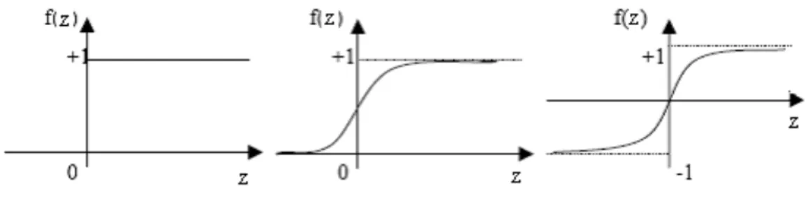
(31) Comparative study of ANN and Box-Jenkins ARIMA for Stock price indexes. 1.4.2.2 – Transfer Function in ANN. The use of transfer function has been indispensable in ANN. Let’s assume in the equation (1.4.13) a function f, the transfer function, defined by. m n  Y j = f  ∑ ∑ β j ( X iα ji ) .  j= 0 i= 0 . €. (1.4.14). The transfer function is responsible for transferring the weighted sum of inputs to some value that is given to the next neuron. There are several types of transfer functions, among which. 1, z > 0 Binary transfer function, f (z) =  , z∈ℜ 0, z ≤ 0. and. 1 Sigmoid transfer function, f (z) = , z∈ℜ. −z €1+ e € Note that the return value of this€functions lies in the interval [0,1], and in consequence these € functions cannot be used in ANN to approximate functions, which can also take negative values (e.g. returns time series). As shown below, in Figure 1.4.3, the binary transfer function and the sigmoid transfer function, are bound between 0 and 1. The difference lies on the fact that the logistic function turns on gradually when activated. When the logistic function approaches 0, the function is almost insensitive to impulse received from input layer, meaning output is inactivated.. sinh(z) e z − e−z = The tangent hyperbolic transfer function, f (z) = , z ∈ ℜ, cosh(z) e z + e−z has the advantage of having the output interval, [-1,1], thus, it can be used in ANN that need € stock index differences). to approximate functions that can take on negative values (e.g. €. 23.

(32) Comparative study of ANN and Box-Jenkins ARIMA for Stock price indexes. Figure 1.4.3: Transfer functions. A wrong functional form of the model under investigation leads to incorrect estimation of parameters. ANN model builders are less concerned about the shape of the function, as specified by the magnitude of the functional parameters. The Neural Networks model parameters are obtained by using the learning algorithms. The success or failure of these learning algorithms depends on whether or not the transfer function is differentiable. The most common nonlinear functions used are the sigmoid function and the tangent hyperbolic function. When the network contains hidden layers the sigmoid function is preferred to binary one, since the latter renders a model difficult to train. In this instance, the error obtained during the training process (which serves in the estimation of parameters) is constant, hence the gradient does not exist or is zero, making the learning process impossible when used some learning algorithms, such as backpropagation. With the sigmoid function it is possible to tell whether the change in weights is good or bad, because a small change in the weights will generate some change in output. With the step unit function, a small change in weights will usually generate no change in output. If the relationship between input units and hidden units is nonlinear, a typical ANN specification consists of approximating the relation by the logistic function. We have then 1. Hj =. n. −. 1+ e. €. .. (1.4.15). ∑ α ij x i i =0. Placing (1.4.15) in (1.4.12), we have. 24.

(33) Comparative study of ANN and Box-Jenkins ARIMA for Stock price indexes. (1.4.16). where f(x) is an identity function, m is the number of hidden units n is the number of input units, α ij are the connection strengths between the input layer and hidden layer, β j represent network weights that connect the hidden layer to the output layer and H(X) is a logistic. €. function connecting the output layer to the input layer.. €. 1.4.2.3 – Learning Rule. The power of Neural Network models depends to a large extent on the way their layer connection weights are adjusted over time. Usually the weights of the ANN must be adjusted using some learning algorithm in order for the ANN to be able to approximate the target function with a sufficient precision. A learning rule is defined as a method that modifies the weights and bias of a network. This method is also known as a training algorithm. The reasoning behind training is that the weights are updated in a way that will facilitate the learning of patterns inherent to the data. Data are divided into two sets, a training set and a test set. The training set serves to estimate weights in the model. Hence, the learning process is a crucial phase in ANN modelling. Usually the test set, is consisting of 10% to 30% of the total data set. The algorithm used to estimate the values of parameters, depends on the type of ANN under investigation.. 1.4.2.4 – Backpropagation learning algorithm. Backpropagation is by far the most popular neural network algorithm that has been used to 25.

(34) Comparative study of ANN and Box-Jenkins ARIMA for Stock price indexes. perform training on multi-layer feedforward neural networks. It is a method for transmission responsibility for mismatches to each of the processing elements in the network by propagating the gradient of the activation function back through the network to each hidden layer down to the first hidden layer. The weights ( ω1,ω 2 ,…,ω n ) are then modified so as to minimize the mean squared error between the network prediction and the actual target.. € In other words, the network processes an output, which depends on the networks weights, (that initially are assigned random values – usually between -1 and 1), input units, hidden units and the transfer function. The difference between the process and actual output (target), known as network error is propagating backward into the network. This error is used to update weights. This process is repeated until the total network error is minimized. The error function can be defined as.  1 N E(ω ) = ∑ (Tt − Yt ) 2 2 t=1. (1.4.17). where Tt and Yt are the targeted output value and the process output in the t th iteration, €  respectively, i.e., E(ω ) is the sum of prediction errors for all training examples.. €. € € Prediction errors of individual training examples are in turn equal to the sum of the €  differences between output values produced by the ANN and the desired (correct) values. ω. is the vector containing the weights of the ANN. The goal of a learning algorithm is to  minimize E(ω ) for a particular set of training examples. There are several ways to achieve € this, one common way is using the gradient descendent method. €. 1.4.2.4.1 – Stochastic gradient descent backpropagation learning algorithm. The gradient descendent method, can be described by 4 steps:. 26.

(35) Comparative study of ANN and Box-Jenkins ARIMA for Stock price indexes. • First Step: choose some random initial values for the model parameters.  • Second Step: calculate the gradient of the error function ∇E(ω ) :  ∂E(ω ) ∂E(ω ) ∂E(ω )  ∇E(ω ) =  , ,…, . ∂ω n   ∂ω1 ∂ω 2 € • Third Step: change the model parameters so that we move a short distance in the  direction of the greatest rate of decrease of the error, i.e., in the direction of - ∇E(ω ) €  • Fourth Step: Repeat second and third steps until ∇E(ω ) gets close to zero. If the. gradient of E is negative, we must increase ω to move ”forward” towards the minimum. € If E is positive, we must move ”backwards”€to the minimum. € First, a neural network is created and initialized (weights are set to small random numbers).. Then, until the termination condition (e.g. the mean squared error of the ANN is less than a certain error threshold) is met, all training examples are ”taught” by the ANN. Inputs of each training example are fed to the ANN, and processed from the input layer, over the hidden layer(s) to the output layer. In this way, vector Yt of output values produced by the ANN is obtained (third step). In the next step, the weights of the ANN must be adjusted. Basically, this happens when the weight update value, Δω , must ”move” the weight in the direction of € steepest descent of the error function E with respect to the weight, or the partial derivative of E with respect to the weight:. Δω = −η. €. €. €. ∂E ∂ω ji. (1.4.18). where η is the learning rate that determines the size of the step that it is used for “moving” towards the minimum of E. If it is too small, then the convergence to optimal point may be small, leading to a slow convergence of ANN. Conversely, if it is too large, the algorithm may not converge at all. Usually η ∈ ℜ, 0 ≤ η ≤ 1. Note that ω ji can influence the ANN only through net, i.e., the weighted sum of inputs for € unit j , therefore, we can use the chain rule to write. € €. ∂E ∂E ∂net j = ∂ω ji ∂net j ∂ω ji. .. (1.4.19) 27. €.

(36) Comparative study of ANN and Box-Jenkins ARIMA for Stock price indexes. Notes that. ∂net j = (net j )dω ji ∂ω ji   (net j )dω ji = ∑ω jz x jz dω ji = (ω j 0 .x j 0 +  + ω jz .x jz ) dω ji  z  = (0.x j 0 +  + 1.x ji +  + 0.x jz ) = x ji . So the equation (1.4.19) it is reduced to. € ∂E ∂E = x ji . ∂ω ji ∂net j. €. (1.4.20). The weights of hidden nodes are also updated. All the expressions are the same for both output and hidden nodes, with the exception of the derivation of δ j =. ∂E . ∂net j. In the case of output nodes, net j , they can influenced ANN only through Y j . Similarly it was € done above, with ω ji , we can chain rule to write:. € ∂E ∂E ∂Y j = € ∂net j ∂Y j ∂net j. €. € .. (1.4.21). Note that  ∂E  1 1 =  ∑ (T j − Y j ) 2 dY j = ((T0 − Y0 ) 2 +  + (Tz − Yz ) 2 ) dY j ∂Y j  2 z 2  1 = (0 +  + (−2T j + 2Y j ) +  + 0) 2 = −(T j − Y j ). ∂Y j ∂transfer(net j ) = = transfer' (net j ) . ∂net j ∂net j. €. 28.

(37) Comparative study of ANN and Box-Jenkins ARIMA for Stock price indexes. So the equation (1.4.21) it is reduced to. ∂E = −(T j − Y j ).transfer' (net j ) ∂net j. €. .. (1.4.22). Considering the previous equations, the weight update Δω for output nodes can be expressed as:. Δω = −η. ∂E ∂E ∂net j = −η = ∂ω ji ∂net j ∂ω ji = −η. €. ∂E ∂Y j x ji = ∂Y j ∂net j. = −η(−(T j − Y j ))( transfer' (net j )) x ji = = η(T j − Y j )( transfer' (net j )) x ji. .. For hidden nodes, this derivation must take into account the indirect ways in which ω ji can. €. influence the network outputs, consequently E.. € There are many improvements of this algorithm such as momentum term, weight decay etc.. However, multilayer feedback in combination with stochastic gradient descent learning algorithm is the most popular ANN technique used in practice. Another important feature of this learning algorithm is that it assumes a quadratic error function, hence it assumes there is only one minimum. In practice, the error function can have - apart from the global minimum multiple local minima. There is a danger for the algorithm to land in one of the local minima and thus not be able to reduce the error to highest extent possible by reaching a global minimum.. 29.

(38) Comparative study of ANN and Box-Jenkins ARIMA for Stock price indexes. Chapter 2. 2 – INPUT DATA, MODELS SELECTION AND RESULTS. 2.1 – DATA AND SOME DESCRIPTIVE STATISTICS. The data, used in this study are extracted from Thomson Financial Datastream and correspond to stock price indexes for four countries namely: Germany (BD), Italy (IT), Greece (GR) and Portugal (PT). The observations are daily time series and are ranged from February 1st 1991 to February 1st, 2006, which yields a total of n = 4175 observations for each series. In the following table it is possible to see some descriptive statistics of the four time series, including the Jarque-Bera Test of Normality. We do reject the null hypothesis that the residuals are normally distributed in all time series.. Figure 2.1: Descriptive statistics. 30.

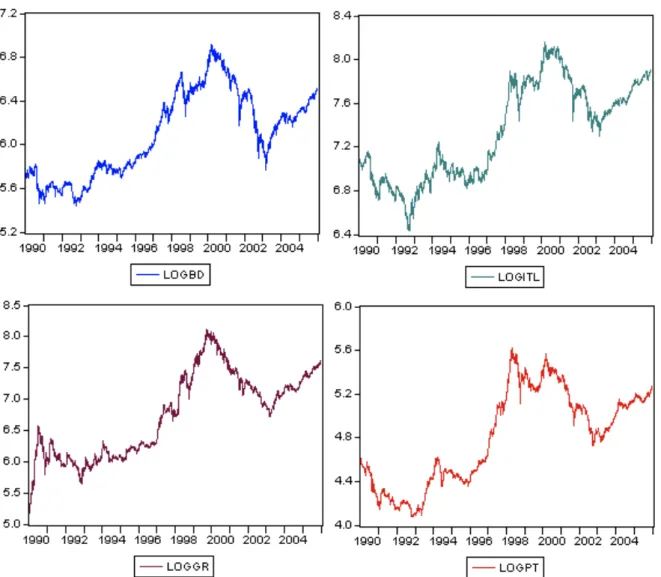
(39) Comparative study of ANN and Box-Jenkins ARIMA for Stock price indexes. As these time series represent stock price indexes, the original data were transformed using the natural logarithm, also in order to reduce the effect of outliers. One of the main advantage of such transformation is the stationary property; which permit to not lose the important information from trading, and it is also transforming the data to stabilize the variance. Thus, the daily time series were coded as: LOGBD= natural logarithm of the Stock price index of Germany: TOTMKBD(PI), LOGITL= natural logarithm of the Stock price index of Italy: TOTMKIT(PI), LOGGR= natural logarithm of the Stock price index of Greece: TOTMKGR(PI) and LOGPT= natural logarithm of the Stock price index of Portugal: TOTMKPT(PI). There are several testes for stationary, but the most encountered in the literature are those related with graphical analyses, correlograms and the unit root test Figure 2.2, depict the nonstationary shape of each one of the four time series, it is going to be analyse. These series varies randomly over time and there is no global trend or seasonality observed. All of them have a quite similar behaviour during all observed period, with a steepest decrease of Italy in the 90th justifying the socio-political conditions and with a consistent increasing for Greece after 90th which can be justified by the collapse of communism in the Balkanians. A decreasing for all of them after 2000 is justifying by the terrorist attacks on September 2001, as well as ,the subsequent terrorist attacks.. 31.

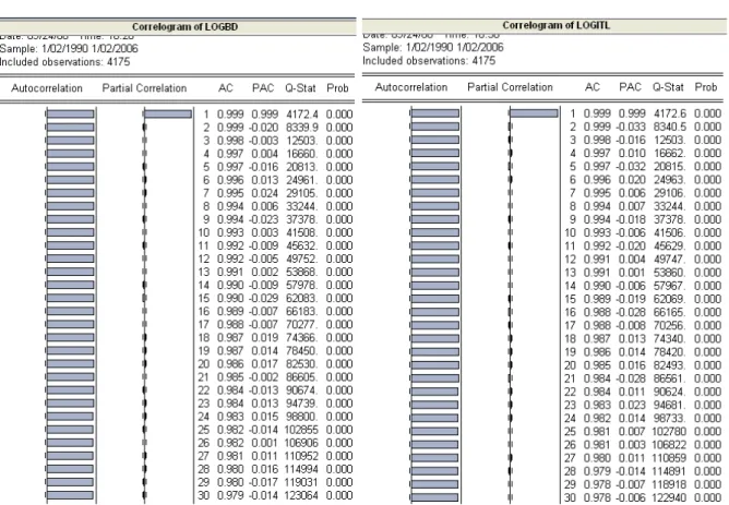
(40) Comparative study of ANN and Box-Jenkins ARIMA for Stock price indexes. Figure 2.2: Graphical representation of natural logarithm of the four Stock price index.. When regarding a correlogram we can find if a particular time series is stationary. For this purpose it is consider the correlogram of natural logarithm series (figure 2.3 and 2.4) and, the correlogram of first difference of natural logarithm series on figures 2.6 and 2.7, where it is shown the correlogram up to 30 lags for each time series.. 32.

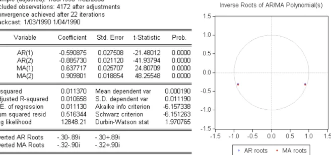
(41) Comparative study of ANN and Box-Jenkins ARIMA for Stock price indexes. Figure 2.3: The correlogram of LOGBD and the correlogram of LOGGR. Figure 2.4: The correlogram of LOGITL and the correlogram of LOGPT. 33.