E
CONOMETRIA
A
PLICADA E
P
REVISÃO
T
RABALHO
F
INAL DE
M
ESTRADO
D
ISSERTAÇÃO
P
REDICTING
A
GGREGATE
R
ETURNS
USING
V
ALUATION
R
ATIOS
O
UT
-
OF
-S
AMPLE
A
NA
C
ARLA
N
ATAL DA
S
ILVA
S
EQUEIRA
M
ESTRADO EM
E
CONOMETRIA
A
PLICADA E
P
REVISÃO
T
RABALHO
F
INAL DE
M
ESTRADO
D
ISSERTAÇÃO
P
REDICTING
A
GGREGATE
R
ETURNS
USING
V
ALUATION
R
ATIOS
O
UT
-
OF
-S
AMPLE
A
NA
C
ARLA
N
ATAL DA
S
ILVA
S
EQUEIRA
O
RIENTAÇÃO:
J
OÃOV
ALLE EA
ZEVEDO,
B
ANCO DEP
ORTUGALi
A
BSTRACT
It is well established that valuation ratios provide, in-sample, relevant signals regarding
future returns on assets. This pattern of predictability is pervasive across financial
markets. In this dissertation we assess the ability of valuation ratios to predict
out-of-sample aggregate returns for the stock and the housing markets in the U.S.. We apply
linear models and multivariate filters to produce the forecasts and employ powerful
out-of-sample tests for inference. We find that there is statistical evidence supporting
the extension of the in-sample results to an out-of-sample framework. The
dividend-price ratio and the rent-dividend-price ratio display a significant ability for predicting stock and
housing returns, respectively. Nevertheless, we note that these findings may be
sample dependent. Especially for the stock market, the end of the sample, including
the recent financial crisis, may be responsible for the good results.
ii
R
ESUMO
É amplamente reconhecido que os valuation ratios fornecem, in-sample, indicações
relevantes sobre os retornos futuros de ativos. Este padrão de previsibilidade é comum
a uma larga maioria de mercados. Nesta dissertação, avaliamos a capacidade de certos
valuation ratios para prever, out-of-sample, os retornos agregados para o mercado de
ações e para o mercado imobiliário, nos E.U.A.. Aplicamos modelos lineares e filtros
multivariados para gerar as previsões e utilizamos “poderosos” testes out-of-sample
para fazer inferência estatística. Verificamos que existe evidência estatística que
suporta a passagem dos resultados in-sample para um contexto out-of-sample. O rácio
dividendo-preço e o rácio renda-preço apresentam uma capacidade significativa para
prever os retornos de ações e imóveis, respetivamente. Notamos, contudo, que estes
resultados podem depender da amostra. Sobretudo para o mercado de ações, o final
da amostra (que inclui a recente crise financeira) pode ser o responsável pelos bons
resultados.
iii
A
CKNOWLEDGMENTS
I would like to thank my advisor João Valle e Azevedo for his entire availability, ideas
and relevant observations, as well as for the constant support and motivation. I am
also grateful to Ana Pereira for providing me her valuable programming
codes and clarifying some questions, Martín Saldías for his important suggestions and
Mário Centeno for his comprehension. I owe an appreciation to the Bank of Portugal,
particularly to the Research Department, that provided all the necessary conditions to
successfully develop this dissertation.
Special thanks go to Hugo for his patience and continuous support, ideas and fruitful
discussions and for his reviews and constructive comments. I would also like to thank
my master colleagues, particularly Luís, for their vital encouragement and helpful
remarks.
Finally, I wish to express my deep gratitude to my family for their unconditional
support.
Thank you all.
iv
C
ONTENTS
1. Introduction... 1
2. A Brief Review of the Relevant Literature ... 3
3. In-Sample and Out-of-Sample ... 5
4. Data ... 8
5. In-Sample Fit ... 10
6. Econometric Procedure ... 11
6.1. Predictive regression models ... 12
6.2. Estimation period ... 15
6.3. Forecast evaluation ... 16
6.4. Out-of-Sample tests ... 18
6.4.1. Equal Accuracy test ... 19
6.4.2. Forecast Encompassing tests ... 22
6.5. Bootstrap procedure ... 26
7. Empirical Results ... 27
8. Future Research ... 32
9. Conclusion ... 33
References ... 34
Appendix A – Figures ... 38
Appendix B – Tables ... 46
v
L
IST OF
F
IGURES
vi
L
IST OF
T
ABLES
Table I Descriptive Statistics ... 46
Table II In-Sample Regressions (horizons of 1, 4, 6, 8, 12, 18, 20 and 24 quarters)... 46
Table III MSFE ratios and Equal Accuracy test results for the stock market (horizons of 1, 4, 6, 8, 12, 18, 20 and 24 quarters). ... 47
Table IV Forecast Encompassing test results for the stock market (horizons of 1, 4, 6, 8, 12, 18, 20 and 24 quarters). ... 47
Table V MSFE ratios and Equal Accuracy test results for the housing market using CSW data (horizons of 1, 4, 6, 8, 12, 18, 20 and 24 quarters). ... 48
Table VI MSFE ratios and Equal Accuracy test results for the housing market using OFHEO data (horizons of 1, 4, 6, 8, 12, 18, 20 and 24 quarters). ... 48
Table VII Forecast Encompassing test results for the housing market using CSW data (horizons of 1, 4, 6, 8, 12, 18, 20 and 24 quarters). ... 49
1
1.
I
NTRODUCTION
Predicting returns is one of the most discussed topics in the academic financial world.
Cochrane (2011) summarizes a pattern of predictability that is pervasive across
markets. For a wide set of markets (stocks, bonds, houses, credit spreads, foreign
exchange and sovereign debt), he concludes (in-sample) that a yield or a valuation
ratio predicts excess returns, instead of cashflow or price change.1 For the stock
market, Cochrane (2011) argues that the dividend yields predict returns and do not
predict dividend growth. More than that, low dividend-yield ratios mean low future
returns and high dividend-yield ratios mean high future returns. For the housing
market, the argument is similar: high prices, relative to rents, imply low returns, and
do not signal the permanent increase of rents or prices.
From an asset pricing perspective, we can explain this phenomenon using the
fundamental present value relation. That is, the price of a financial asset should equal
the present value of its future cashflows or, briefly, asset prices should equal expected
discounted cashflows. In the case of the housing market, this means that the price of a
house should equal the present value of its future rents (the analogy to the stock
market is straightforward). This relation then implies that observed fluctuations in
financial asset prices should reflect variation in future cashflow, in future discount
rates, or in both.
1 See, Fama and French (1988, 1989) for stocks; Fama and Bliss (1987), Campbell and Shiller (1991) and
2
In this paper, we intend to verify whether this pervasive phenomenon holds
out-of-sample, i.e., whether a forecaster would be able to predict excess returns
systematically, if he stood at the forecast moment without further information. Since
there are relatively few studies about predicting the housing returns, we decided to
focus on the housing market. The stock market analysis appears as an important
reference. We use linear models and multivariate filters to produce the forecasts for
the two aforementioned markets and employ equal accuracy tests and forecast
encompassing tests for inference.
Our results show that there is statistical evidence supporting the extension of the
in-sample results to an out-of-sample framework. Especially for the housing market,
we conclude that the rent-price ratio has a huge ability for predicting returns
(performing the equal accuracy test, we note that all the values are statistically
different from at the significance level).
Given the lack of out-of-sample studies for the housing market, we consider that
our findings are a considerable contribution to the literature. Using a diverse set of
models to produce the forecasts of returns, we also apply relatively powerful test
statistics and a bootstrap approach (because our models are nested) to conduct robust
inference. We obtain all the results for the housing market using two different data
sources (the Case-Shiller-Weiss (CSW) index and the Office of Federal Housing
Enterprise Oversight (OFHEO) price index).
As Rapach and Wohar (2006), our purpose is testing for the existence of return
3
“whether a practitioner in real time could have constructed a portfolio that earns
extra-normal returns”.
The remainder of this paper is organized as follows. In Section 2 we briefly review
the relevant literature and in Section 3 we provide a theoretical distinction between
the in-sample and out-of-sample concepts. Section 4 describes the data used to obtain
the empirical results, while Section 5 reports the in-sample results. In Section 6 we
expose the econometric methodology. Section 7 discusses our main findings and the
last two sections present ideas for future research and the conclusions.
2.
A
B
RIEF
R
EVIEW OF THE
R
ELEVANT
L
ITERATURE
As mentioned before, there are about a handful of papers examining the predictability
of housing returns. Case and Shiller (1990) investigate the prices and excess returns
(in-sample) predictability in the housing market based on a set of independent
variables including the rent-price ratio. For this variable, the estimated coefficient in
the ordinary least squares (OLS) regression is positive and statistically significant.
Using quarterly data and based on a long-horizon regression, Gallin (2008) shows
that changes in real rents tend to be larger than usual and changes in real prices tend
to be smaller than usual, when house prices are high relative to rents.
With a different focus, Campbell (2009) apply the dynamic Gordon growth
model to the housing market and find that changes in expected future housing premia
4
More recently, Plazzi (2010) conclude (in-sample) that the rent-price ratio
predicts expected returns for apartments, retail properties and industrial properties
(but does not predict expected returns of office buildings).
For the stock market, the literature is voluminous. Several authors have already
examined the ability of the most common financial variables to be good predictors for
the aggregate returns or the equity premium.
Goyal and Welch (2003) assess the performance of the dividend-price ratio when
used to predict the CRSP (Center for Research in Security Prices) value-weighted
annual excess returns. Contrary to the in-sample results, they find that the
out-of-sample forecasts produced through a model with the dividend-price ratio have a worse
performance than those created by a model of constant returns (that is, a model that
includes only the constant term).
Along the same line, Goyal and Welch (2008) explore the existence of gains when
one uses the financial variables with a reasonable in-sample performance to forecast
(out-of-sample) the equity premium. They conclude that almost all models produce
poor results out-of-sample, which suggest “that most models are unstable or even
spurious”.
Against this background, Rapach and Wohar (2006), using annual data over the
period, conclude that several financial variables have a good in-sample
and out-of-sample ability to forecast stock returns. As justification for these results,
they emphasize the fact that the tests employed are robust for inference (specifically,
5
Following a slightly different approach, Rapach (2010) use forecast combining
methods to produce out-of-sample forecasts and find that this approach provides
significant out-of-sample gains when compared to the historical mean.
3.
I
N
-S
AMPLE AND
O
UT
-
OF
-S
AMPLE
Although we aim at exploring out-of-sample forecasts, we consider important to
understand the differences between in-sample predictability and out-of-sample
predictability. In this section, we will distinguish these concepts.
For sake of simplicity, let us consider the following regression model:
where is the return from holding the financial asset from until , is
the forecast horizon, is the financial variable used to predict and is a
disturbance term.
An in-sample analysis consists of estimating the equation using the available
observations and then, examine the associated to the OLS
estimate of and the goodness-of-fit measure to assess the predictive ability of
.2 When the null hypothesis is rejected and the is high, we can conclude that
has predictive power over .
There are some potential problems related to this perspective, specifically the
small-sample bias ( is not an exogenous regressor in equation ; see Stambaugh
2 The null hypothesis (
6
(1986, 1999)) and the dependence between the observations for the regressand in
(these observations are overlapping when the forecast horizon is greater than ; see
Richardson and Stock (1989)). The serial correlation induced in the disturbance term
should be taken into consideration when conducting inference. The Newey and West
(1987) standard errors robust to the autocorrelation and the heteroskedasticity are a
usual solution.
An out-of-sample analysis implies the generation of the forecasts for . Typically,
the researcher chooses one of the three most common schemes (fixed, recursive or
rolling) that allow producing the predictions in-real time, as if the forecaster stood in
the moment when the prediction is made (i.e. using the data available up to that time).
Here, we describe the concept of out-of-sample predictability only based in the
recursive scheme for this is the scheme we use in our empirical applications.
We should start by determining the sample-split parameter ( ), that is, the period
of the first prediction (we discuss this issue in more detail in Section 6.2.). Once we
obtain predictions for different forecast horizons ( ), determining is not the same as
determining the period of the last observation used in estimating the model (which
will be ). Fixing , we ensure that the first forecast obtained refers to the
same period, for each .
Next, we split the total sample ( observations) into an in-sample portion (includes
the first observations) and an out-of-sample portion (composed of the
7
model (equation , for example). The other allows evaluating the performance of
the obtained forecasts through the analysis of the forecast errors.
Using the OLS estimates of the coefficients in equation , we construct the
forecast for the period given the information until , that is:
And then we compute the forecast error ( for :
where is the observed value of the dependent variable at .
The remaining predictions are obtained by repeating this procedure for
, that is:
In the end, we have forecasts but only forecast
errors. We can then determine the Mean Squared Forecast Error ( ):
and compare the forecasts obtained through the different models (which are
8
4.
D
ATA
In this section, we describe and characterize the data (available at John Cochrane’s
website) used in the models estimation.
Stock Market:
As Lettau and Ludvigson (2001), we use quarterly data for the U.S. stock market.
Our sample covers the period ( ) and our dependent
variable is the equity premium from holding stocks from period to .
As usual, we define equity premium as the return on the stock market minus the
return on a short-term (risk-free) interest rate. In our case, we use the CRSP
value-weighted return less the -month Treasury bill return (the -month Treasury bill is a
proxy for the risk-free rate). Formalizing, we can write the variable to forecast
periods ahead ( as:
where , is the return (including dividends) on the Value-Weighted
Index, and is the -month Treasury bill return.
The dividend-price ratio ( is the financial variable which potentially predicts the
equity premium:
9
We intend to verify whether the pervasive phenomenon identified by Cochrane
(2011) holds out-of-sample. Our variables were therefore constructed following the
definitions presented in Cochrane (2011) we use the simple returns instead of log
returns. At all events, Goyal and Welch (2003) tried both specifications and found
similar conclusions.
Housing Market:
In our applications for the housing market, we use quarterly data from to
( ). There are two different available samples with similar
information. One comes from the Case-Shiller-Weiss (CSW) price data, the other
consists in the houses prices and rents from the Office of Federal Housing Enterprise
Oversight (OFHEO) “purchase-only” price index.
Our dependent variable ( ) is the log return from holding the house from until
and the predictor is the respective rent-price ratio ( . That is:
As mentioned before, for both markets, we construct the variables based on the
10
C).3 Table I in Appendix B contains the usual descriptive statistics for all the analyzed
series.
5.
I
N
-S
AMPLE
F
IT
As mentioned in Goyal and Welch (2008), the out-of-sample performance is only
interesting when the model has a good in-sample performance. Hence, in this section,
we discuss the results obtained through the in-sample regressions and present some
motivations to the out-of-sample exercise.
Table II in Appendix B provides the results of regressing the returns from holding
the financial asset from to ( on the corresponding valuation ratio ( ).
Specifically, for each market in question, we estimate:
where and have the meanings introduced in Section 3; , as before, is the
forecast horizon in quarters.
The equation is estimated by OLS and the Newey and West (1987) standard
errors, which are robust to heteroskedasticity and serial correlation, are used to
compute the . Following Rapach and Wohar (2006), we use the Bartlett
kernel and a lag truncation parameter equal to , where denotes the integer
part, for ; and zero for to calculate these standard errors.
3 The stock market data and the housing market data are available at
11
As mentioned before, we assess the in-sample predictive performance based on
values of the and . We can also interpret the OLS estimate of as an
indicator of the significance to forecast .
Analyzing the results shown in Table II (Appendix B), we can detect a set of
characteristics that are common across the two markets. The estimate of and the
are higher for longer forecast horizons, and the observed always reject
the null hypothesis of no predictability. In addition, the signal of the estimates is
positive, which confirms the conclusions presented in Cochrane (2011): higher
valuation ratios indicate higher returns. Or, more specifically, high prices, relative to
dividends (or rents, for the housing market) can be a sign of low returns.
Hereupon, and since this in-sample predictability may mean nothing out-of-sample,
it is of all the interest to examine the predictability of these variables out-of-sample.
6.
E
CONOMETRIC
P
ROCEDURE
In this section, we discuss the regression models used to produce the out-of-sample
forecasts, the methods employed to compare them and, lastly, the equal accuracy
tests and the forecast encompassing tests applied to statistically analyze the results.
12
6.1. Predictive regression models
Apart from assessing the out-of-sample performance of the valuation ratios to predict
aggregate returns, we also aim at identifying which model(s) provides the best
forecasts compared to the historical mean. Therefore, we select several methods to
generate different sets of predictions for the same variable aggregate returns. All of
them are estimated using OLS.
In what follows, denotes the forecast of (the return from holding the
financial asset from to ), given the information up to period , and is the
valuation ratio that might have predictive power for .
A direct method requires that only information available up to is used to obtain
the forecast for . By contrast, the iterated method generates the prediction
for , using one-step ahead forecasts. For , the direct and the iterated
models produce the same forecasts. The direct approach is computacionally simpler.
• ( ) Historical mean:
As Goyal and Welch (2003, 2008) and Campbell and Thompson (2008), we use the
historical mean as a benchmark forecasting model, since it represents the hypothesis
of no predictability, consistent with the most common interpretation of the efficient
13
• ( ) Direct autoregressive ( ) with fixed lag order ( ):
where and are the OLS estimates. In our empirical applications,
we fix .
• ( ) Direct using the Akaike Information Criterion (AIC) (Akaike, 1974) to
determine the lag order ( ):
In this method, we only define the maximum lag order ( ). After that,
whenever a forecast is generated, we apply the AIC to determine the optimal number
of lags ( ), given all the past information. Thus, for each period , the employed to
produce the prediction can be different.
• ( ) Direct augmented using the AICto determine the lag order ( ):
and are the OLS estimates. The expression
“augmented” denotes the introduction of valuation ratios as explanatory variables in
the regression. Again, the lag order is determined by the AIC (the above comment
14 • ( ) Direct regression with or without lags:
In this method, the autoregressive part is not taken into consideration.
• ( ) Univariate and multivariate filters:
Following the argument presented in Valle e Azevedo and Pereira (2012), when we
choose this method to generate our forecasts, we assume that we are interested in
predicting the low frequencies of (say, , where is a
band-pass filter eliminating the fluctuations with period smaller than a specified
cut-off) and using these predictions as forecasts of itself. Explicitly, we will consider
predictions of the low frequencies of aggregate returns as forecasts of aggregate
returns itself. The weights of the ideal filter ( ) are given by:
Nevertheless, since is an infinite (absolutely summable and stationary)
polynomial in lag operator and we only have available a finite sample ( ), we
approximate the low frequencies of (that is, ) through a weighted sum of
elements of ( ), which will be considered a forecast for . That is:
and denote the number of observations in the past and in the future, respectively,
15
We obtain the multivariate filter when we include, in that weighted sum, elements
of series of covariance-stationary covariates , where
. Namely:
Solving the problem:
where the information set is implicitly restricted by and , we determine (the
weights of the filter are found solving a linear system with
equations and unknowns). The solution to problem is discussed in Valle e Azevedo
(2011).
To extract the signal for , we should set in the
solution. As a result, only the available information up to period is employed.4
After choosing the model, we apply the recursive scheme described in Section 3 to
generate the forecasts.
6.2. Estimation period
As mentioned in Section 3, the first step of an out-of-sample analysis is to determine
the in-sample period and the out-of-sample period. Specifically, we should fix a value
to the sample-split parameter ( ). Nevertheless, there is no criterion that defines how
16
to choose . We should make a compromise between the number of observations
used to estimate the coefficients of the model and the number of available
observations to assess the forecasts performance.
It is natural to compare predictions at different horizons referring to the same
period of time (regardless the forecast horizon). To make this possible, the forecast for
period must be generated based in the information until period , which implies
that, for longer horizons, less observations are available to estimate the coefficients.
Additionally, since we are forecasting the aggregate returns (the returns from
holding the financial asset from until ), we lose the first observations of the
series of interest. Again, longer forecast horizons imply losing more initial
observations.
Taking this information into consideration, we fix , which corresponds to
the first quarter of in the stock market data (we consider the predictions for the
period ) and to the first quarter of in the housing market
data (we consider the predictions for the period ).
6.3. Forecast evaluation
We choose the (out-of-sample) Mean Squared Forecast Error ( ) ratio as
evaluation metric to compare the sets of forecasts obtained through the models
17
Given a set of -step ahead forecasts generated by the model
, we calculate the forecast errors as:
where is the observed value of the dependent variable at and is the forecast
of , generated by model , given the information up to .
Consequently, the for model is equal to:
Denoting the of the benchmark model (the historical mean) by
and the of the competing model by , the ratio is
given by:
When the is less than , the competing model predicts better than the
benchmark model, suggesting that there are out-of-sample forecasting gains.
Otherwise, the historical mean (which signals constant expected returns) is the best
possible forecast.
We also use a graphical analysis to examine the relative performance of the
forecasting models. As proposed in Goyal and Welch (2003), we construct charts with
18
( ) and the cumulative squared forecast errors of the competing model
( ). Formalizing:
When this difference is positive, the competing model outperforms the benchmark
model (the sum of the squared forecast errors from through (i.e., the date in the
-axis) is greater for the benchmark model than for the competing model).
6.4. Out-of-Sample tests
We assess the statistical significance of the obtained results considering equal accuracy
tests (under the null hypothesis, the from two distinct models are statistically
equal) and forecast encompassing tests (we test whether a given set of forecasts
generated by a simpler model embody all the useful predictive information contained
in another set of forecasts).
Before describing these tests in more detail, it is important to make a distinction
between nested and non-nested models and, above all, note that, excluding the
multivariate filter (model ), all of our models are nested.
We say that two models are nested when there is a set of regressors that is
common between them. In our studies, whenever we compare the competing model
with the benchmark model (model ), we are comparing nested models
19
zero in models and , we obtain the model ). Briefly, the benchmark model
(which includes only the constant term) is a restricted version of the model of interest.
This clarification is relevant because, as stressed in Clark and McCracken (2005),
when we have nested models, the population errors of the analyzed models are
exactly the same, under the null hypothesis that the restrictions imposed in the
benchmark model are true. This implies that the asymptotic difference between the
of two models is exactly zero with zero variance and, consequently, the
standard distributions are asymptotically invalid.
Because our models are nested and different forecast horizons ( , in
quarters) are explored, we use, as recommended in literature, a bootstrap procedure
for inference.
6.4.1. Equal Accuracy test
Using the as the evaluation metric, the equal accuracy test allows testing
whether the ratio is statistically equal to , against the alternative that the
forecasts produced by the competing model are better (have a lower ).
Tantamount, we can write:
where is the of the competing model and is the of the
20
Using the set of -steps ahead forecast errors from model , we
can also express the null hypothesis as follows:
where
First proposed by Diebold and Mariano (1995), the test statistic can be
written as:
where:
; ;
is the estimated th autocovariance of :
is the truncation parameter and
is the Bartlett Kernel.
Following Clark and McCracken (2005), we fix for and
for . This test statistic has an asymptotic standard normal distribution when used
21
Notwithstanding, there is evidence that the test could be over-sized for
in small and moderate samples. Thus, Harvey (1997) proposed a
small-sample correction that resulted in the following test statistic:
These authors recommend comparing the values of the modified statistic with critical
values from the Student’s distribution with degrees of freedom, when
comparing forecasts from non nested models.
Due to the emergence of other problems (namely, the degeneracy of the long-run
variance of ), McCracken (2007) develops the test statistic:
where is the of the competing model .
In our case, a significant – statistic means that the forecasts from the
competing model have statistically more predictive power than those from the
historical mean model.
For practical purposes, we will use the and the
test statistics which have non standard distributions with nested models. 5,6 Clark and
McCracken (2001) and McCracken (2007) provide tables with asymptotic critical values
5 Clark and McCracken (2001) find that
has higher power than .
22
for . Since we are interested in a multi-step analysis, we based our inference in a
bootstrap approach (except for the multivariate filter model).
6.4.2. Forecast Encompassing tests
According to Clements and Harvey (2009), a set of forecasts encompasses a rival set if
the latter does not contribute to a statistically significant reduction in when
used in combination with the original set of forecasts. Applying this concept to our
study, if the historical mean forecast encompasses the forecast produced by the model
with the valuation ratio, then the financial variable does not contain useful additional
information for predicting the aggregate returns.
We will present three alternative definitions for forecast encompassing. The way
how the test is applied depends on the chosen setting.
The most general formulation, proposed by Fair and Shiller (1989), considers that
encompasses if the value of is zero in equation:
where denotes the -steps ahead forecast of produced by model (
for the restricted model (historical mean) and for the unrestricted model).
As a result, we should test ( encompasses ) against
23
Assuming that the individual forecasts are efficient, we can impose the restriction
in the equation , obtaining the regression: 7
However, to apply the forecast encompassing test, we consider the Andrews
(1996) approach instead of equation .8 Consequently, the encompassing is defined
by (we test against ) in the regression:
where and .
Finally, dropping the intercept in equation , which means fixing , we
require that the individual forecasts are unbiased and efficient. In this last specification
we define encompassing by in the equation:
As mentioned in Clements and Harvey (2009), if the restrictions imposed (
when the forecasts are unbiased, and when the forecasts are efficient) do
not hold, the exposed definitions are not equivalent, implying that we can take
different conclusions using distinct classifications. Nevertheless, when the restrictions
imposed are true, the tests based in the modified equations ( or ) should be
more powerful.
7 A forecast
is said to be Mincer-Zarnowitz efficient if and in a regression
, which implies no correlation between the forecast and the forecast error.
8 This approach results from some transformations in equation
Specifically,
24
Additionally, if the optimal value of in equation is zero, we should conclude
that, in sense, the forecast of cannot be improved by adding the
forecast in the linear function of (i.e., ), which does not imply that
the is the optimal forecast for .
In order to test for encompassing, the standard cannot be used since
the regression errors may not be independent (we consider ) nor normally
distributed.9,10 Therefore, Harvey (1998) proposed an approach, based in
Diebold and Mariano (1995) test statistic, which consists in testing whether the series
( is the number of forecast errors from each model) has zero mean. The test
statistic is similar to that presented in Section 6.4.1 for the equal accuracy test,
changing just the definition of which depends on the regression ( or ).
The following table describes the three possible cases: 11
Characteristics of the individual forecasts
Biased and Inefficient: Regression
Biased and Efficient: Regression Unbiased and Efficient: Regression
where and denote the errors from regressions of and , respectively, on a constant and ; and .
9 Note that the optimal forecast errors is expected to follow a moving-average process of order
.
10 Harvey
(1998) examine this problem in the context of unbiased and efficient individual forecasts.
25
Formally, the test statistic is given by:
where and have the aforementioned meaning. We can also compute the
modified approach suggested by Harvey (1997).
Clark and McCracken (2001, 2005), admitting that the individual forecasts are
unbiased and efficient, developed the following test statistic:
which is more powerful than the previous test statistics for forecast encompassing.12
The test statistics exposed do not have a standard distribution (and, most often,
neither a pivotal asymptotic distribution) in the case of multi-step predictions. The
procedure of obtaining forecasts using estimated regression models (the estimation
uncertainty affects the encompassing tests) and the existence of nested models also
difficult the deduction of the critical values. Therefore, it is widely suggested in the
literature to use the critical values generated by bootstrap methods.
In our practical application, we employ the and the
statistics to test the forecast encompassing. The critical values used are obtained by
bootstrapping.
12 Clark and McCracken (2001) provide the critical values for this test statistic, when
26
6.5. Bootstrap procedure
We follow Mark (1995) and Kilian (1999) to define a bootstrap method which allows
obtaining the critical values for the test statistics described in previous sections.
As Goyal and Welch (2008), we impose the null hypothesis of no predictability
assuming that the data generating process (DGP) is:
where denotes the aggregate returns and is the predictor. We estimate the
equations and by , using the full sample. 13
The next step is to generate (we set ) innovation sequences, of length
, by drawing randomly with replacement from fitted residuals and
( ). Using the sequences
and ( ) and the OLS
coefficient estimates obtained in first step, we produce sequences of observations
for and . Specifically, for , we construct:
Since follows an autoregressive process of order , we need an initial
observation, namely, an observation that is prior to sample used to estimate the
13 We could use the seemingly unrelated regressions (SUR) to estimate these equations. However, the
27
equations. Whenever necessary, this observation will be randomly selected by picking
one date from the available data.
Finally, for each set of observations, we apply the recursive scheme described in
Section 3. In the end, we will have sets of forecasts and sets of
the corresponding forecast errors. After calculating the values of the test statistics (we
have observed values for each statistic test), we determine the , and
critical values as the , and percentiles of the resulting statistics,
respectively.
7.
E
MPIRICAL
R
ESULTS
In this section, we expose and discuss the main results obtained using the
methodology described before. This analysis will be done separately for each market.
We first present the findings for the stock market (specifically, the results of the
out-of-sample statistical tests and the interpretation of the charts), and then we
do the same for the housing market.14
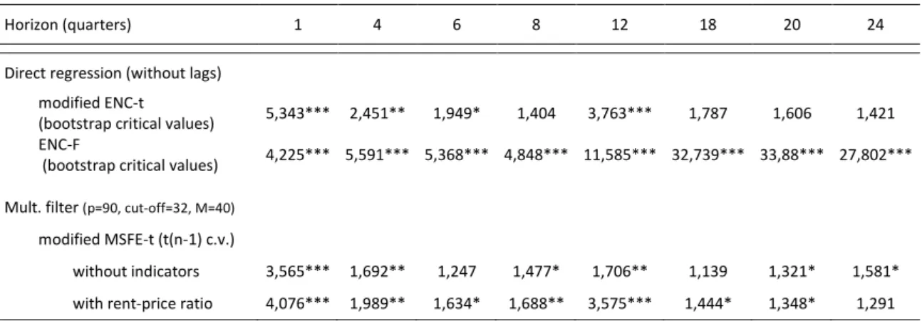
Stock Market:
Although we have generated forecasts using different models, we only statistically
analyze those obtained by the direct regression model (model without lags) and
multivariate filter (model using the dividend-price ratio), since these are the
models that produce better results. As the benchmark (the historical mean) and the
14
28
direct regression are nested models, we use the bootstrap critical values to perform
the out-of-sample tests.
Table III in Appendix B reports the ratios for each model. We conclude that
only the direct regression generates forecasts that can beat the benchmark for all
horizons. These ratios are statistically different from at conventional significance
levels when we use the statistic (equation ) to perform the equal
accuracy test. Both the quality and the statistical significance of the predictions
increase with the forecast horizon, which suggests that the dividend–price ratio ability
to predict the aggregate returns improves when we use longer horizons. These findings
are consistent with the in-sample results exposed in Section 5, where we note that the
in-sample predictability increases with the horizon.
The univariate filter model failed to outperform the benchmark model for all
horizons, but the multivariate filter has ratios less than for and
(despite not being statistically different from 1 when we use the
statistic (equation ) to apply the test).
Similar conclusions can be drawn when we analyze the forecast encompassing
results presented in Table IV, Appendix B (which contains the observed values of the
test statistics). In particular, when we use the (equation ) to perform the
test, we have statistical evidence to reject the null hypothesis (the historical mean
forecasts encompass those produced by direct regression model) at a significance
29
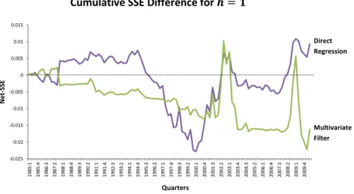
The following analysis rests on the evaluation of the charts
which display the cumulative squared forecast errors of the
benchmark model (from 1985:Q1 through the date in the -axis) minus the squared
forecast errors of the competing model (from 1985:Q1 trough the date in the -axis),
for each horizon. A positive value means that the competing model has outperformed
the benchmark model and a positive slope indicates that the competing model had
lower forecasting error than the historical mean model, in a given quarter.
For the stock market, we chose to plot merely the
for the direct regression model (without lags) and the
multivariate filter model (with dividend-price ratio) since these illustrate the main
findings.
Considering the shorter forecast horizon ( quarter, see figure ), we note that the
direct regression curve exhibits a volatile pattern. This competing model had a good
performance in , and
and had its poorest performance from to (although it
begins to recover (the curve has a positive slope) from ). For , the
multivariate filter consistently has a worse performance than the direct regression
model.
Figure also shows the cumulative difference for , when both models
underperformed the benchmark. For this horizon, the dividend-price ratio model had
30
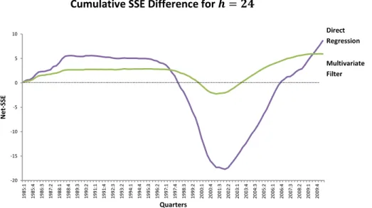
For longer forecast horizons ( , for example; see figure in Appendix A), the
curves are smoother and we can identify three distinct periods (which have become
more apparent as the horizon increases). Namely: an initial period when the forecasts
produced by the competing models are better, an intermediate period when the
models had a negative performance and a final period of recovery. We note that this
final period may be responsible for the good results out-of-sample, meaning that if we
dropped the last observations of the sample, the direct regression model probably
could not beat the benchmark. It is also worth noticing that the direct regression
model curve has an extremer behavior than the multivariate filter curve, that is, it had
the best performance but also has the worst in given portions of the sample.
Housing Market:
As we mentioned in Section 4, we have two data sources for the housing market.
The results are quite similar.
Tables V and VI in Appendix B contain the ratios between the competing and
the benchmark model for horizons . For
forecast horizons shorter than years ( quarters), we find that all the competing
models produce better forecasts than the benchmark model. However, and
importantly, for longer horizons (over years), only the models that contain the
rent-price ratio exhibit ratios lower than .
In particular, the ratio between the direct regression and the benchmark
31
statistic (equation ) to conduct the equal accuracy test, we note that all the values
are statistically different from (at the significance level). Comparing with the
results obtained in Section 5, we verify that the predictability pattern identified
in-sample holds out-of-in-sample for the housing market.
As regards to the multivariate filter, we observe that, although the ratios are
always lower than , we only have statistical significance for . Tables VII and VIII
(in Appendix B) display the forecast encompassing statistics for concluding that the
historical mean forecasts never encompass the forecasts generated by the direct
regression model (the null hypothesis is always rejected at a significance level of ).
Figures 2 and 3 in Appendix A contain the charts with the
for the CSW data and the OFHEO data. We only examine the curves
from three models: the direct model (with ), the direct augmented
model (also with ) and the direct regression model (without lags). Although
we choose to show the charts based on the two data sources, we note that there are
few differences between them (we will do a general analysis).
Examining the figures 2 and 3, for , we conclude that the direct regression
model had mild underperformance from to , conversely it had a
superior performance in the rest of the sample. The other two models exhibit a really
good performance from to (before that, the is almost
zero for both models).
When we consider the forecast horizons of and quarters, the competing
32
models that include the rent-price ratio start to exhibit a better performance than the
model with only the autoregressive component. This pattern is obvious when we
analyze the figures 2 and 3, for and , where the cumulative
difference between the and the benchmark model is constantly negative. From
, the direct regression curve grows almost exponentially, evidencing the
predictive power of the rent-price ratio.
8.
F
UTURE
R
ESEARCH
In this section, we propose ideas for future research, some of which are improvements
to our paper.
An obvious gap in our study is the lack of robust critical values to statistically assess
the quality of forecasts produced by the autoregressive models (which are also nested
models). To solve this problem, it should be defined a bootstrap procedure that
generate this critical values under the null hypothesis of no predictability.
Additionally, it would be interesting to extend this research to other markets,
namely the bonds, the treasuries, the sovereign debt or the foreign debt markets.
There are relatively few papers about predicting returns of these markets, out-of
sample. Another suggestion would be to reproduce this study using data for the
European markets instead of to the U.S. markets.
From a financial perspective, and since our results reveal that the valuation ratios
33
markets, an academic researcher could also explore the existence of profitable
investment strategies.
9.
C
ONCLUSION
In this dissertation, we found evidence that the known in-sample pattern of return
predictability across markets holds out-of-sample. Considering the stock and the
housing market, we verify that there are gains when we use valuation ratios to predict
aggregate returns. The relatively powerful out-of-sample tests applied corroborate
these results. In particular, for the stock market, we found that the direct regression
model beats the benchmark, for all horizons. Additionally, we note that the dividend–
price ratio’s ability to predict the aggregate returns improves at longer horizons. For
the housing market, only the models that contain the rent-price ratio consistently
exhibit ratios lower than , for all horizons.
The sample dependence identified through the analysis of charts, for both
markets, deserves further attention. It will be interesting to investigate this issue in
detail, notably by examining the stability of the forecast function while linking it to
34
R
EFERENCES
[1] Andrews, M. J., Minford, A. P. L. and Riley, J. (1996). “On comparing macroeconomic forecasts using forecast encompassing tests”. Oxford Bulletin of Economics and Statistics,
, pp. .
[2] Akaike, H. (1974). “A new look at the statistical model identification''. IEEE Transactions on Automatic Control, , pp. .
[3] Calhoun, C. (1996). “OFHEO house price indices: HPI technical description”. From:
http://www.ofheo.gov (Retrieved September 17, 2012)
[4] Campbell, J. Y. and Shiller, R. J. (1991). “Yield spreads and interest rate movements: A
bird’s eye view”. Review of Economic Studies, , pp. – .
[5] Campbell, J. Y. and Thompson, S. B. (2008). “Predicting excess stock returns out of sample:
Can anything beat the historical average?”. Review of Financial Studies, , pp.
— .
[6] Campbell, S. D., Davis, M. A., Gallin, J. and Martin, R. F. (2009). “What Moves Housing Markets: A Trend and Variance Decomposition of the Rent-price Ratio”. Journal of Urban Economics, , pp. – .
[7] Case, K. E. and Shiller, R. J. (1990). “Forecasting Prices and Excess Returns in the Housing
Market”. Real Estate Economics, , pp. – .
[8] Clark, T. E. and McCracken, M. W. (2001). “Tests of Equal Forecast Accuracy and Encompassing for Nested Models”. Journal of Econometrics, , pp. – .
[9] Clark, T. E., and McCracken, M. W. (2005). “Evaluating direct multi-step forecasts”.
35
[10] Cochrane, J. (2011). “Discount Rates”. Journal of Finance, , pp. .
[11] Clements, M. P. and Harvey, D. I. (2009). “Forecast Combination and Encompassing”. In: Mills, T.C. and Patterson, K., (Eds.) Palgrave Handbook of Econometrics, Volume : Applied Econometrics Palgrave Macmillan, pp. .
[12] Diebold, F. X. and Mariano, R. S. (1995). “Comparing predictive accuracy”. Journal of Business and Economic Statistics, , pp. .
[13] Fair, R. C. and Shiller, R. J. (1989). “The informational content of ex ante forecasts”. Review of Economics and Statistics, , pp. .
[14] Fama, E. F. (1984). “Forward and spot exchange rates”. Journal of Monetary Economics,
, pp. .
[15] Fama, E. F. (1986). “Term premiums and default premiums in money markets”. Journal of Financial Economics, , pp. – .
[16] Fama, E. F. and Bliss, R. R. (1987). “The information in long-maturity forward rates”.
American Economic Review, , pp. – .
[17] Fama, E. F. and French, K. R. (1988). “Dividend yields and expected stock returns”. Journal of Financial Economics, , pp. – .
[18] Fama, E. F. and French, K. R. (1989). “Business conditions and expected returns on stocks
and bonds”. Journal of Financial Economics, , pp. – .
[19] Gallin, J. (2008). “The long-run relationship between house prices and rents”. Real Estate Economics, , pp. .
36
[21] Goyal, A. and Welch, I. (2003). “Predicting the equity premium with dividend ratios”.
Management Science, , pp. – .
[22] Goyal, A. and Welch, I. (2008). “A Comprehensive Look at the Empirical Performance of
Equity Premium Predictions”. Review of Financial Studies, , pp. – .
[23] Hansen, L. P. and Hodrick, R. J. (1980). “Forward exchange rates as optimal predictors of future spot rates: An econometric analysis”. Journal of Political Economy, , pp.
– .
[24] Harvey, D. I., Leybourne, S. and Newbold, P. (1997). “Testing the equality of prediction
mean squared errors”. International Journal of Forecasting, , pp.
[25] Harvey, D. I., Leybourne, S. and Newbold, P. (1998). “Tests for forecast encompassing”.
Journal of Business and Economic Statistics, , pp. .
[26] Kilian, L. (1999). “Exchange rates and monetary fundamentals: what do we learn from
long–horizon regressions?”. Journal of Applied Econometrics, , pp. – .
[27] Lettau, M. and Ludvigson, S. C. (2001). “Consumption, Aggregate Wealth, and Expected
Stock Returns”. Journal of Finance, , pp. – .
[28] Mark, N. C. (1995). “Exchange rates and fundamentals: evidence on long–horizon
predictability”. American Economic Review, , pp. – .
[29] McCracken, M. W. (2007). “Asymptotics for Out of Sample Tests of Granger Causality”.
Journal of Econometrics, , pp. – .
37
[31] Piazzesi, M. and Swanson, E. (2008). “Futures prices as risk-adjusted forecasts of monetary
policy”. Journal of Monetary Economics, , pp. – .
[32] Plazzi, A., Torous, W. and Valkanov, R. (2010). “Expected Returns and the Expected Growth
in Rents of Commercial Real Estate”. Review of Financial Studies, , pp.
.
[33] Rapach, D. and Wohar, M. (2006). “In-Sample vs. Out-of-Sample Tests of Stock Return
Predictability in the Context of Data Mining”. Journal of Empirical Finance, , pp.
– .
[34] Rapach, D., Strauss, J. and Zhou, G. (2010). “Out-of-Sample Equity Premium Prediction:
Combination Forecasts and Links to the Real Economy.” Review of Financial Studies, , pp. .
[35] Richardson, M. and Stock, J. H. (1989). “Drawing inferences from statistics based on
multiyear asset returns”. Journal of Financial Economics, , pp. – .
[36] Stambaugh, R. F. (1986). “Biases in regressions with lagged stochastic regressors”. Graduate School of Business, University of Chicago, Working Paper .
[37] Stambaugh, R. F. (1999). “Predictive regressions”. Journal of Financial Economics, , pp.
– .
[38] Valle e Azevedo, J. (2011). “A Multivariate Band-Pass filter for Economic Time Series”,
Journal of the Royal Statistical Society (C), , pp. .
38 -0.025 -0.02 -0.015 -0.01 -0.005 0 0.005 0.01 0.015
1985:1 1985:4 1986:3 1987:2 1988:1 1988:4 1989:3 1990:2 1991:1 1991:4 1992:3 1993:2 1994:1 1994:4 1995:3 1996:2 1997:1 1997:4 1998:3 1999:2 2000:1 2000:4 2001:3 2002:2 2003:1 2003:4 2004:3 2005:2 2006:1 2006:4 2007:3 2008:2 2009:1 2009:4
Net -SSE Quarters -0.6 -0.5 -0.4 -0.3 -0.2 -0.1 0 0.1 0.2
1985:1 1985:4 1986:3 1987:2 1988:1 1988:4 1989:3 1990:2 1991:1 1991:4 1992:3 1993:2 1994:1 1994:4 1995:3 1996:2 1997:1 1997:4 1998:3 1999:2 2000:1 2000:4 2001:3 2002:2 2003:1 2003:4 2004:3 2005:2 2006:1 2006:4 2007:3 2008:2 2009:1 2009:4
Net
-SSE
Quarters
A
PPENDIX
A
–
F
IGURES
Figure 1. Cumulative SSE Difference charts for the Stock Market (horizons of 1, 4, 8, 12, 18
and 24 quarters).
Notes: This figure plots the for , that is, the cumulative squared forecast errors of the benchmark model (the historical mean) minus the squared forecast errors of the
competing model, for each horizon. We consider two competing models: the direct regression model
(purple curve) and the multivariate filter model (green curve). A positive value means that the
competing model has outperformed the benchmark model. A positive slope indicates that the
competing model had lower forecasting error than the historical mean model, in a given quarter.
Cumulative SSE Difference for
Cumulative SSE Difference for
LA S EQ UE IR A | P R EDIC TIN G A G G R EG A TE R ET U R N S US IN G V A LUA TIO N R A TIO S O UT -OF -S A MPL E 39 39 -2
.5 -2 -1.5 -1 -0.5 0 0.5
1985:1 1985:4 1986:3 1987:2 1988:1 1988:4 1989:3 1990:2 1991:1 1991:4 1992:3 1993:2 1994:1 1994:4 1995:3 1996:2 1997:1 1997:4 1998:3 1999:2 2000:1 2000:4 2001:3 2002:2 2003:1 2003:4 2004:3 2005:2 2006:1 2006:4 2007:3 2008:2 2009:1 2009:4 Net-SSE Q ua rte rs
-5 -4 -3 -2 -1 0 1
1985:1 1985:4 1986:3 1987:2 1988:1 1988:4 1989:3 1990:2 1991:1 1991:4 1992:3 1993:2 1994:1 1994:4 1995:3 1996:2 1997:1 1997:4 1998:3 1999:2 2000:1 2000:4 2001:3 2002:2 2003:1 2003:4 2004:3 2005:2 2006:1 2006:4 2007:3 2008:2 2009:1 2009:4 Net-SSE Q ua rte rs
-12 -10 -8 -6 -4 -2
0 2 4
40 -20 -15 -10 -5 0 5 10
1985:1 1985:4 1986:3 1987:2 1988:1 1988:4 1989:3 1990:2 1991:1 1991:4 1992:3 1993:2 1994:1 1994:4 1995:3 1996:2 1997:1 1997:4 1998:3 1999:2 2000:1 2000:4 2001:3 2002:2 2003:1 2003:4 2004:3 2005:2 2006:1 2006:4 2007:3 2008:2 2009:1 2009:4
Net -SSE Quarters -0.005 0 0.005 0.01 0.015 0.02 0.025 0.03 0.035 0.04 Net -SSE Quarters
Cumulative SSE Difference for
Figure 2. Cumulative SSE Difference charts for the Housing Market using CSW data (horizons
of 1, 4, 8, 12, 18 and 24 quarters).
Notes: This figure plots the for , that is, the cumulative squared forecast errors of the benchmark model (the historical mean) minus the squared forecast errors of the
competing model, for each horizon. We consider three competing models: the direct regression model
without lags (green curve), the direct autoregressive ( ) model (purple curve) and the direct
augmented model (red curve). The lag order of the models with autoregressive component is
determined by the Akaike Information Criterion ( ). A positive value means that the competing
model has outperformed the benchmark model. A positive slope indicates that the competing model
had lower forecasting error than the historical mean model, in a given quarter.
Cumulative SSE Difference for
41 -0.1 0 0.1 0.2 0.3 0.4 0.5 Net -SSE Quarters -0.6 -0.4 -0.2 0 0.2 0.4 0.6 0.8 1 Net -SSE Quarters -1 -0.5 0 0.5 1 1.5 Net -SSE Quarters
Cumulative SSE Difference for
Cumulative SSE Difference for
Cumulative SSE Difference for