The impact of brazilian crisis on export and non-export stocks

(1)

THE IMPACT OF BRAZILIAN CRISIS ON EXPORT AND

NON-EXPORT STOCKS

Frederico Augusto Fogolin Pereira

(2)

THE IMPACT OF BRAZILIAN CRISIS ON EXPORT AND

NON-EXPORT STOCKS

Frederico Augusto Fogolin Pereira

Project submitted as partial requirement for the conferral of MSc in Business

Management

Supervisor:

Prof. Doutor José Dias Curto, Associate Professor, ISCTE-IUL Business School,

Department of Quantitative Methods

(3)

PEREIRA, Frederico Augusto Fogolin. The impact of Brazilian crisis on export and

non-export stocks. Project submitted as partial requirement for the conferral of MSc in Business

Management. Lisboa: ISCTE – Business School, 2017.

ABSTRACT

Considering that Brazil is currently one of the major emerging economies in the world through this work is possible to compare the returns of before and after the 2015 crisis peak (GDP = -3.8%) with the evolution of the principal stock exchange in Brazil (IBOVESPA). As known, the exchange rate is the major source of macroeconomic uncertainty is important to understand if the export companies have a higher profitability than non-export companies. As basis for this work, I used the 407 companies listed in IBOVESPA, being separated between: Exporters and Non-Exporters. The analysis continued using Log Return and in the end, I was able to prove that the differences in the daily returns of the companies that export are statistically higher than those that do not export, making it clear that even in a critical period like 2014 to 2016 it is possible profitability vis-à-vis non-exporters.

(4)

PEREIRA, Frederico Augusto Fogolin. O impacto da crise brasileira sobre estoques de

exportação e não-exportação. Projeto apresentado como requisito parcial para a atribuição de

Mestrado em Gestão Empresarial (Mestre em Gestão Empresarial). Instituto Universitário de Lisboa - ISCTE – Business School, 2017.

RESUMO

Considerando que o Brasil é atualmente uma das principais economias emergentes do mundo através deste trabalho é possível comparar os retornos de antes e após o pico de crise de 2015 (PIB = -3,8%) com a evolução da bolsa no Brasil (IBOVESPA). Como é sabido, a taxa de câmbio é a principal fonte de incerteza macroeconômica e é importante para entender se as empresas de exportação têm uma maior rentabilidade do que as empresas não-exportadoras. Como base para este trabalho, usei as 407 empresas listadas no IBOVESPA, sendo separadas entre: exportadoras e não exportadoras. A análise continuou usando Log Return e, no final, eu consegui provar que as diferenças nos rendimentos diários das empresas que exportam são estatisticamente superiores às que não exportam, deixando claro que mesmo em um período crítico como 2014 para 2016 é possível uma maior rentabilidade em relação aos não exportadores.

(5)

LISTA DE ABREVIATURAS

AELP3 Aes Elpa-Energy

BMTO4 Brasmotor-Manufacturer of Refrigeration Compressors BNDES Brazilian Development Bank

BPHA3 Brasil Pharma-Pharmaceuticals BRIN3 BR Insurance-Insurance Brocker BRKM5 Braskem AS-Chemical Company BRL/USD Reais/United State Dollar

BRML3 BR Malls- Holding

CASN3 Companhia Catarinense de Agua e Saneamento-Water Supply COCE5 Companhia Energética do Ceára-Energy

CPLE3 Copel-Energy

CSAN3 Cosan-Energy

CTAX3 Contax-Third Party Services CTIP3 Cetip-Financial Market CTNM3 Cotemias-Fabric Manufacture

ECPR3 Empresa Nacional de Comércio Crédito- Credit FESA4 Alloy Iron CIA of Bahia-Mining and Metallurgy FIBR3 Fibria Celulose AS-Pulp

GDP Gross Domestic Product HETA4 Hercules AS-Cutlery Factory HGTX3 CIA Hering- Clothing Manufacturer HOOT4 Hoteis Othon- Hotel

HUNIP6 Unipar Cabocloro-Chemical Company

IBGE Brazilian Institute of Geography and Statistics IBOVESPA São Paulo Stock Exchange

JBSS3 JBS-Food

JOPA3 Josapar-Food

LAME4 Lojas Americanas Retailer

LIXC4 Construtora Lix da Cunha-Buildings

LUPA3 Lupatech- Equipaments and Services for Oil and Gas MIDIA3 ML Dias Branco- Food

PIB Produto Interno Bruto PMAM3 Paranapanema AS-Copper RADL3 Raia Drogasil-Pharmaceutical SBUB34 Starbucks-Coffee Shop SELIC SELIC base interest rate

TCNO4 Tecnosolo Engenharia-Engineering Consulting TPIS3 Triunfo Participações-Services

(6)

INDEX OF FIGURE

Figure 1 – Brazil takes off – Special report...14

Figure 2 – Has Brazil blown it? Special report...15

Figure 3 – 2 Variance comparison test – Exporters: Before X During Crisis...36

Figure 4 – 2 Variance comparison test – Non-Exporters: Before X During Crisis...37

Figure 5 – 2 Sample t test – Exporters: Before X During Crisis...38

Figure 6 – 2 Sample t test – Non-Exporters: Before X During Crisis...38

Figure 7 – 2 Variance comparison test – Exporters X Non-Exporters: 2011 to 2016...39

(7)

INDEX OF GRAPHS

Graph 1 – Slump in the Real...16

Graph 2 – IBOVESPA Index of analyzed companies...23

Graph 3 – Annual Brazilian GDP...23

Graph 4 – Times Series – Returns – Higher Std. Deviation...25

Graph 5 – Times Series – Returns – Lower Std. Deviation...26

Graph 8 – IBOVESPA X BRL/USD...30

(8)

INDEX OF TABLES

Table 1 – Exporters – Descriptive Statistics...24

Table 2 – Non Exporters – Descriptive Statistics...27

Table 3 – Exporters – Descriptive Statistics...30

Table 4 – Non Exporters – Descriptive Statistics...33

(9)

ACKNOWLEDGMENTS

I wish to thank to all of those who contributed either directly or indirectly to this work.

To my mother Claudete and Daniela, my wife, who always supported me during this challenge, no matter what.

To my supervisor Professor Dr. José Dias Curto, for his mentoring and for giving me total freedom of thought and actions. Also showing me that statistics is not a monster and can be easily explain to anyone, it is just matter of a good history!

(10)

INDEX

1 INTRODUCTION...11

1.1 RESEARCH PROBLEM ... ...16

1.2 OBJETIVES ...17

2 LITERATURE REVIEW...18

2.1 EXPORT VERSUS NON-EXPORTING COMPANIES ... 18

3 METHODOLOGY...20 4 EMPIRICAL ANALYSIS...23 4.1 BEFORE CRISIS ... ...24 4.1.1 Exporters ...24 4.1.2 Non - Exporters ...26 4.2 DURING CRISIS ... ...29 4.2.1 Exporters ...29 4.2.2 Non - Exporters ...33 5 COMPARATIVE ANALYSIS...36 6 CONCLUSIONS...41 7 BIBLIOGRAPHY...43

(11)

1 INTRODUCTION

A recent research in econophysics has shown that financial markets can be considered as complex systems due to a large number of agent’s interactions, stimulating the research on characteristics of price fluctuations in financial markets (Tabak, et.al, 2009). In Brazil, they are mostly from commodity or financial sector, described on IBOVESPA, the main point for data gathering used to make decisions. It´s a gross total return index weighted by traded volume and is comprised of the most liquid stocks traded on São Paulo stock exchange.

As the values changes among time, there are some researchers studying the movements in aggregate stock market volatility. Officer (1973) said that these changes are related to the volatility of macroeconomic variables. Black (1976) and Christie (1982) argue that financial leverage partially explains this phenomenon. Merton (1980), Mascaro and Meltzer (1983), Pindyck (1984), Poterba and Summers (1986), French, Schwert, and Stambaugh (1987), Bollerslev, Engle (1982), and Wooldridge (1988), Abel (1988) and Lauterbach (1989) find that macroeconomic volatility is highly related to interest rates from investors.

When the investors put money in the stock market, they want to look at profitability from a specific company. But this is not the only factor to be observed, since a risk and return analysis is necessary. Sometimes the most profitable company does not correspond to the high risk to be accepted. This risk in turn is defined as the chance of the return of an initial investment to be different than expected, culminating in the total or partial loss of the amount applied.

A concept associated with risk is Volatility, which can be defined as: A statistical measure of the possibility of the asset rendering or giving damage in a certain period of time. Such volatility is commonly analyzed with the use of variance or standard deviation, using historical data from a company. This measure changes according to the stipulated period of time, that is, the period chosen is highly influential.

Therefore, this variable is named as the leading indicator of stock returns and according to Binder and Merges (2001), the state that the volatility of the return on the market portfolio is inversely related to the ratio of expected profits to expected revenues for the economy. Nardari and Scruggs (2005) infer that high uncertainty regarding future returns are mainly associated with recessions or crisis and during this period the stock market volatility could be higher (Schwert,1989). However, Moore (1983) and Schwert (1989) indicate stock prices as leading indicators, reporting that the turn in stock prices takes place prior to the turn in business activity movement, especially for local markets or emerging economies that are not well prepared for surpass the bad period.

(12)

Matos et.al (2014) said that Brazil is characterized by diversity in its macroeconomic and financial strategies, trying for more than 50 years of attempts to constitute new commercial and monetary blocks. Therefore, with a positive trend when analyzed the whole period of time and the economic development as a whole.

There is a name used in literature to refer on that moment of crisis, which is “contagion”. It is a spread of market changes or disturbances from one regional market to others. We can also refer to the economic crises throughout a geographic region.

After a huge shock to one country, some fundamental reasons are explicit to increase in cross-market linkages. Some researches refer to “pure contagion” which cannot be explained by changes in fundamentals. A pure contagion is defined as a significant increase in cross-market correlations and relates to shifts in investors interest to take a risk. When this appetite for risk falls, they instantly reduce their exposure to risky assets and fall in value together. In other hand, when the appetite rises, demand for risky assets increase and their value rise at the same time. Therefore, this type of contagion runs a part of the lines of risk and rid of fundamentals, trade and exchange rate arrangements (Kumar & Persaud, 2001).

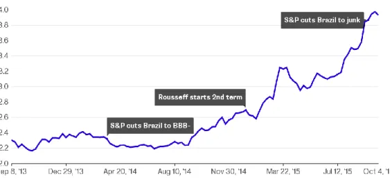
The current environment in Brazil is unsustainable as it is in the second consecutive year of recession, reaching a GDP of -3,6% in 2016.

In 2011, when the president of the republic, Dilma Rousseff assumed the presidency, she and her economic team openly declared that Brazil would adopt a "New Economic Matrix". It was based on five pillars:

1º) Expansionary fiscal policy

This policy is adopted when the objective is to stimulate aggregate demand, especially when there is a recessionary period and if a government contribution is necessary. Some common guidelines are:

a) Increase public spending and consequently increase production, reducing unemployment. With this increase in public spending, national income also increases, as there is a greater demand for labor and production increases.

b) Reduce the tax burden, having a direct impact on consumer purchasing power and corporate investment.

And since everything has a negative side, the expansionary fiscal policy affects the budget of the Union, generating a deficit that must be covered by the government with the issuance of bonds, increasing the public debt.

(13)

2º) Low interest

The interest rate is the percent of principal charged by the lender for the use of its money. The principal is the amount of money lent. Banks pay you an interest rate on deposits because they borrow that money from you. (Amadeo, 2017).

The interest rate used to be applied to the total unpaid amount of your loan. It's extremely important to know what your interest rate is and how much it adds to your debt.

Therefore, interest rates are not the same as its depends on the bank charge higher interest rates if it thinks there's a lower chance the debt will get paid.

3º) Subsidized credit

This is a benefit given to the people, businesses or institutions by the government. In this case the subsidy is given to remove some kind of burden and promote a social good or an economic.

4º) Depreciated exchange rate

A exchange rate can be beneficial if the economy is uncompetitive and stuck in a recession. A devaluation helps to increased demand for exports and create jobs. In a recession, inflation is unlikely to be a problem. However, in a boom, a devaluation could lead to inflation. Also, a devaluation does reduce living standards as imports become more expensive (Pettinger, 2013).

It is fundamental to have an appreciation in the exchange rate and see its beneficiates. If there is an appreciation due to speculation, then it could be harmful as exporters will not be able to compete.

5º) Increase in import tariffs to stimulate domestic industry

The federal government will raise import taxes to protect the domestic industry, from which they can increase their taxes by up to 25%, for a fixed term of 12 months. The tariff high limit is up to 35%, following the maximum established in the World Trade Organization (WTO). However, all these pillars caused growing budget deficits, import tariffs reached their highest post-real level, BNDES subsidies reached historical highs, the SELIC rate was maintained for six months at its lowest since the “Plano Real”, the exchange rate devaluation was almost as sharp as that of the 2008 crisis, and the population's debt reached record levels (Roque, 2013).

(14)

However, there is no clear consensus among experts about the causes of this recession and the causes are:

Internal

One year before the start of the crisis, in 2013, the British magazine The Economist had already made criticisms to the economic management of the government, having released a 14-page report. The article contrasts two different scenarios in the Brazilian economy, such as:

1 - The country signaled a very promising future when registering a growth of 7.5% in 2010, performing the best results in decades.

2 - Brazil was chosen to host both the 2014 World Cup and the 2016 Olympics which in the future will drain resources from public sector.

The cover below from “The Economist”, shows the good moment for Brazilian economy in 2009:

Figure 1 – Brazil takes off – Special report

Source: The Economist, 2009.

External

Later on, in 2015, The Economist stated that the immediate causes of the crisis were external. The publication says that President Dilma Rousseff could have made better use of the commodity wave to reduce the swollen state. Instead, the chosen direction was to secure subsidized loans and costly tax incentives for some industries. After 4 years, during 2013 a new cover was launch, showing what was the starting point for one of the major crisis in Brazil.

(15)

Figure 2 – Has Brazil blown it? – Special report

Source: The Economist, 2013.

During 2014, the growth in Brazil started to decelerated in what was once one of the fastest-growing economies in the world. The Latin America’s largest economy shrank 3.81 % in 2015, the steepest plunge since 1990, when Brazil was battling the called “hyperinflation”. The International Monetary Fund predicts an improvement, but still with 3.54 % in 2016. Brazil is heading to suffer its worst recession in a century.

According to what we referred before, the purpose of our study is to understand if even in the middle of a crisis, is possible to revert the market instability.

This study will use data from the IBOVESPA, index of the São Paulo Stock Exchange from every company listed. The values will be collected from the companies starting in Jan/2011 to June/2016.

The available information from 427 firms suggests that in 2015 the major negative performance is coming from two companies, Petrobras and Vale, whose shares are highly representative in the IBOVESPA. The oil company, which is experiencing one of its worst crises with Operation “Lava Jato” and loss of investment capacity. In the case of Vale, which suffers from falling commodity prices and the impact of the accident in Mariana (MG), the loss was even worse.

In the midst of its deepest economic and political crisis in a generation, Brazil is contending with a climate so punishing that projects across numerous sectors are being frozen or shrunk, while small businesses reduce prices and shift their focus. (Bloomberg SITE, 2015).

(16)

growth through a positive impact on net exports.

Graphic 1 – Slump in the Real

Source: Performance of the currency – Bloomberg.

Despite the effect of the devaluation on the price of the product the exchange devaluation ended up stimulating production, making the products more competitive for the foreign markets. As an example of the benefit caused by the devaluation, the coffee crop increased in the demand for inputs, which reflected more job creation in the field. The percentage increase was 14.92% (Rodrigues et.al, 2005).

The economic openness explains that an economy could be affected by external shocks, reflection of losses in export revenues. Therefore, the scale of impact depends on the degree of concentration of a country’s export portfolio (Briguglio, 2009, Rodrik 2010, World Bank 2010) in addition with what Basile, 2001 said: "Generally, indeed, large changes in exchange rates are strongly correlated with large changes of export flows of a country” (pag.1186-1201)

1.1 RESEARCH PROBLEM

Variability in exchange rate is the major source of macroeconomic uncertainty that affects all companies. After the 70’s, a quick expansion in international trade and the usage of floating exchange rate regimes by countries, made the exchange rate volatility increase (Yucel and Kurt, 2003).

According to Blecker (2010), countries with a high vulnerability to an international competition and those who imports and exports are price-sensitive as they are less likely to pursue strongly wage-led growth regimes.

(17)

be affected (positive) by the same devaluation once their expenses are in local currency and its revenues comes in foreign currency. The local value share may increase despite any negative effects of the crisis.

The alternative strategy for that is a competitiveness effect, where the internationalization of production suppressed by the local market is the possible exit found by companies.

For that reason is important to understand if the export companies have a higher profitability in the stock market than non-export companies, also during periods of crisis and also because there is not study about the 2014 crisis in Brazil, for that reason this thesis aims to add the currently literature.

1.2 OBJECTIVES

This thesis studies compares the performance of exporting and non-exporting companies in the Brazilian stock market during and after the crisis. Considering that Brazil is currently one of the major emerging economies in the world through this work is possible to compare the returns of before and after the 2015 crisis peak ( GDP=-3,8%) with the evolution of the principal stock exchange in Brazil (IBOVESPA), in order to determine the level of impact in our market.

I will extend the current literature focusing on the main issue:

Are the returns from Brazilian companies that export and those who do not export economically/statistically significant different during and after the crisis period? In other words, we will identify if the adaptation of some local industries to export had a positive effect on their income, before and after the most recent Brazilian economic contraction.

This thesis proceeds as follows. In section one I provide a literature review of the three main topics discussed, namely the export versus non-exporting companies. Section two, the used methodology. Section three is going to be used to describe all data I have, while section four applies methodologies presented before. The next section (5) is Empirical results which contains the interpretation of results. Section six offers a comparative analysis. Section seven aim to add some insight about risk and volatility. Finally, section eight concludes with bibliography.

(18)

2 LITERATURE REVIEW

2.1 EXPORT VERSUS NON-EXPORTING COMPANIES

In 1995, Bernard and Jensen has published one of the firsts studies for exporters and non-exporters companies and still in the top as commented by Wagner 2007; Schröder and Sørensen, 2012; Girma 2014 and Vu, Holmes, Lim and Tran 2014. Based on that, several studies appeared for countries around the world, such as Colombia, Mexico and Marroco (Clerides S., Lauch, S. & Tybout, J.R.1998), UK (Girma, 2014), Chile (Herzer, 2006) and Turkey (Yucel and Kurt, 2003). The literature review shows that at least two gears can explain a positive correlation between the export status of a company and its productivity, self-selection and “learning-by-exporting”. A more productive firm that engages in export activities is able to compete in international markets and enter into export markets, gaining knowledge and experience, allowing then to increase the efficiency level (Loecker, 2005).

According to Vernon (1966), Krugman (1979) and Grossman & Helpman (1991), export product diversification increases long-term growth. Additionally to it in 1999, Bernard and Jensen said that exporters are larger, more productive, more capital-intensive, more technology-intensive, and pay higher wages.

When we talk about the Brazilian case, Ellery Jr. & Gomes, 2005 pointed that we must take in count the stylized facts identified by Tybout (2003): exporters are in the minority, more productive, and have a trend to export a portion of what they produce. Feenstra and Kee (2008); Pöschl et al. (2009) showed evidences that export diversity increases local country productivity and that all companies have heterogeneity and an exceptional characteristic/performance for exporting firms compared to non-exporters. Also the benefits can vary depending on the country location.

According to Blecker (2010) countries with a high vulnerability to an international competition and those who imports and exports are price-sensitive as they are less likely to pursue strongly wage-led growth regimes. They prefer to use a profit-led growth regime when it is compared to the closed economies.

The growth since 2002 was largely based on those firms which already exported (Araujo e Pianto, 2010). According to Dixit (1989) and Krugman (1989) that hysteresis in exports may be due to the sunk costs.

(19)

On 2004, Girma said that exporters have higher productivity than non-exporters supporting contributions from Roberts and Tybout (1996), Clerides, Lach and Tybout (1998), Bernard and Jensen (1999), Alvarez and Lopez (2004).

To be successful on this task, the manufacturer must standardize their domestic products in order to fill foreign customer specifications. New markets, investments and sourcing opportunities will “pop-up” from multinational firms (Garten,1997). A higher exposure to competition and also the possibility of benchmarking with other companies in order to add value to the productive chain (Aw & Hwang 1995, Clerides et al.1998).

The politicians are also convinced that helping exporters is a no-lose issue due to a simple sentence: exports are good, and exporters are good companies, helping domestic firms to export is a good policy (Bernard, 2004).

Hwanc & Aw, 1995, also argued that developing countries that pursue export-oriented trade policies generally outperform due to more inputs, or because they have a greater access, than their counterparts in the domestic market. Contrasting with what was said by (Bekaert & Harvey, 1998), expected companies returns can decrease after a significant breaks in capital flows.

(20)

3 METHODOLOGY

The focus of this thesis is how a country crisis affects stocks values from companies that are exporting and those non-exporting. The period considered was from January 2011 to June 2016 and since 2014, the Brazilian economy began to slow down.

For that reason we are going to perform an empirical analysis of the stock prices on the IBOVESPA index of the São Paulo Stock Exchange in order to test if the stocks of export companies had a better performance than the non-export companies.

During this study the analysis will be with the closing market prices (not adjusted for dividends) for some stocks listed on IBOVESPA traded daily before/after the most recent crisis, starting on Jan/2011 until June/2016.

To go further, it´s usual to compute two measures: Pt and Pt-1 if there is no dividend distribution.

Pt = End of period price

The next step will be the stratification between exporters and non-exporters by looking into the IBOVESPA database or searching for the specific companies. Also split the period above between before and after crisis.

In order to respond to the objectives presented before, we will consider descriptive statistics measures namely mean, variance, standard deviation and coefficient of variation. In order to test if the means and variances are statistically different between exporters and non exporters companies before/after crisis, we will consider the independent samples t test and the Levene test, respectively. Next we present a brief description of the tests.

Descriptive Statistics

Descriptive statistics are numbers that summarize and describe the datasets. They only "describe" the data and do not represent generalizations of the sample to the population. Also can be divided into measures of central tendency and dispersion: the first is used to represent all the values collected in a survey and the second uses a value that reveals how the data varies around that value that is more typical.

The main measures of central tendency that we are going to use in the work are: average and median and the main measures of dispersion are: variance and standard deviation.

(21)

count the total number of cases / results (referred to as n). Afterwards, we must add up all the scores and divide by the total number of cases. On the other hand, there is a disadvantage because it is affected by high or low discrepant scores that distort the desired information to be transmitted over the analyzed data.

The median differs from the mean because it is the average value in the distribution when the values are organized in ascending order. Since we take random values as: 11, 12, 13, 14, and 15, we will have a median of 13. Since it is not influenced by discrepant values, it should be preferred when they are present.

The variance (σ2) is defined as the sum of the squared distances of each term in the distribution from the mean (μ), divided by the number of terms in the distribution (N). In probability theory and statistics, the variance of a random variable or stochastic process is a measure of its statistical dispersion, indicating "how far" in general its values are from the expected value.

Standard deviation is one of the most widely used statistical measures to demonstrate

data variability as it estimates the degree to which the value of a particular variable deviates from the mean. In mathematical terms, the square root of the variance is the standard deviation.

It is given by the equation below.

Mean comparison (2 sample t)

This test is used to determine whether the means of two independent groups differ. In example, you want to determine whether two stock returns are giving more return in the same period of time.

2-Sample t calculates a confidence interval and does a hypothesis test of the difference between two population means when standard deviations are unknown and samples are drawn independently from each other. To do a 2-sample t-test, the two samples must be independent; in other words, the observations from the first sample must not have any bearing on the observations from the second sample.

For 2-Sample t, the hypotheses are: Null hypothesis => H0: μ1- μ2 = δ0

The difference between the population means (μ1- μ2) equals the hypothesized difference (δ0).

(22)

Alternative hypothesis => H1: μ1- μ2≠ δ0

The difference between the population means (μ1- μ2) does not equal the hypothesized difference (δ0). In our case, as the purpose is to test if the means are the same, = δ0.

To calculate it, the formula is as follows:

Levene´s test relies on a method for robust comparison of variances. Given the two

groups of observations xij , i = 1, 2, j = 1,...,ni, the main idea was to define a new variable zij = |xij − ¯xi|, where x¯i is a measure of central tendency, such as the mean or median.

(23)

4 EMPIRICAL ANALYSIS

In total, 392 companies were analyzed in the IBOVESPA index from Jan/2011 to 06/10/2016, of which:

Graphic 2 – IBOVESPA Index of analyzed companies

Source: Author

After that, they were separated in 2 periods, before crisis with the period starting in 2011 and ending in Dec/2013 & After crisis, starting from Jan/2014 to Jun/2016.

That choice was made following the annual Brazilian GDP change according to IBGE and is shown below.

Graphic 3 – Annual Brazilian GDP

Source: IBGE Annual Brazilian GDP

Error - No data available Exporting Companies Non-Exporting Companies Category 163; 41,6% Non-Exporting Companies 147; 37,5% Exporting Companies 82; 20,9%

Error - No data available

(24)

The chart above shows a clearly negative trend starting in 2011 and the sharp decline started in 2013. In 2014, the economy contracted by 2.5% with 2013 and in 2015 reach -3,8% culminating to be the worst GDP level since 1990. A small improvement of 0.2% evaluated in 2016. With that, the effects of the economic crisis were perceived by the population that adapted to the new financial reality. As an example, consumers exchanged essential products for cheaper ones or awaited settlements.

During this year, 2017, GDP raise 1% in Q1, the first increase after consecutive quarterly declines. According to Henrique Meirelles (Finance Minister), “the country left the biggest recession of the century" (BRASIL, 2017).

4.1 BEFORE CRISIS

4.1.1 Exporters

To begin our analysis and to understand what happened in terms of returns, here follows a descriptive analysis of the 147 companies that entered in the Exporting category.

As mentioned before, the log return was used in calculation to create the baseline.

Table 1 - Exporters – Descriptive Statistics

Analysis # of companies

(Total = 147) %

Mean > Median 65 43,90%

Positive Mean 65 43,90%

Source: Author

As can be seen from the table above, 65 companies (43.90%) presented the mean variation above the median and the same amount presented a positive mean. That difference with Mean>Median represents a shift to the right (positive tail) with a positive kurtosis, which is consistent with literature.

The positive mean demonstrate that those 65 companies have a higher return in comparison with the other 82(average).

To continue, we must understand the standard deviation, previously described, as it is significantly higher in some companies, such as:

(25)

HETA4 - Hercules SA - Cutlery factory INEP4 - INEPAR - Telecom

CTKA4 – Karsten – Textile Industry RCSL4 - Recrusul – Road implements

Let's look more closely at each of the companies cited above, exemplifying the high daily variation of returns. Each point in the graph represents a data point of the log return.

Graph 4 – Times Series – Returns – Higher Std.Deviation

Source: Author, font IBOVESPA, 2011-2013

The profiles of the four plots are similar with an oscillating pattern. Also it shows that we have seasonality in the daily returns for HETA4 and INEP4, the year of 2012.

For HETA4, there was a 24% increase in sales compared to 2011. For INEP4, a loss of R$ 76 million.

Now, let's understand how companies that presented a very low Std.Deviation

740 666 592 518 444 370 296 222 148 74 1 400 300 200 100 0 -100 -200 -300 -400 Data Points H ET A 4

Time Series Plot of HETA4

740 666 592 518 444 370 296 222 148 74 1 300 200 100 0 -100 -200 -300 Data Points IN EP 4

Time Series Plot of INEP4

740 666 592 518 444 370 296 222 148 74 1 300 200 100 0 -100 -200 -300 Data Points C T K A 4

Time Series Plot of CTKA4

740 666 592 518 444 370 296 222 148 74 1 500 400 300 200 100 0 -100 -200 -300 -400 Data Points R C S L4

(26)

performed. As example:

VERZ34 - Verizon - Telecom

EXXO34 – Exxon Mobil – Oil & Gas MTSA3 - Metisa - Metalurgy

CATP34 - Caterpillar - Machinery

Graph 5 – Times Series – Returns – Lower Std.Deviation

Source: Author, font (IBOVESPA, 2011-2013)

As noted above, the behaviors are completely different from each. They show a low dispersion of data, however, the EXXO34 shows a great variation starting in 2013. This variation is due to the company's increase in profit in the 3rd and 4th quarter, reaching 5.8% in relation to the previous period.

4.1.2 Non Exporters

The following analysis will be made with the 163 companies not listed as exporter, said that, let's look at table 2 (descriptive statistics) during the same period, before the crisis, for companies that do not export and understand their behavior.

550 495 440 385 330 275 220 165 110 55 1 15 10 5 0 -5 -10 Data Points V ER Z 3 4

Time Series Plot of VERZ34

550 495 440 385 330 275 220 165 110 55 1 12,5 10,0 7,5 5,0 2,5 0,0 -2,5 -5,0 Data Points EX X O 3 4

Time Series Plot of EXXO34

550 495 440 385 330 275 220 165 110 55 1 25 20 15 10 5 0 -5 -10 Data Points M T S A 3

Time Series Plot of MTSA3

550 495 440 385 330 275 220 165 110 55 1 15 10 5 0 -5 -10 Data Points C A T P 3 4

(27)

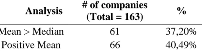
Table 2 – Non Exporters – Descriptive Statistics

(Total = 163) %

As can be seen from the table above, 61 companies (37.2%) presented the mean variation above the median as well a left skew. A difference of 6.7% in relation to the companies that export.

It generates greater profitability in exports for the cases of companies that closed the exchange on days when the national currency depreciates. With this, we can affirm that the expected volatility of the exchange affected the profitability of the exporters, in the case of those who converted the dollar to the national currency in that period.

Now, let´s continue with the coefficient of variation, in order to check the data dispersion for the top four, such as:

BRIN3 – BR Insurance – Insurance

RJCP3 – RJ Capital Partners – Financial Mngt. TCNO4 – Tecnosolo – Engineering

HOOT4 – Hoteis Othon - Hotel

Let's look more closely with a time series analysis for each of the companies cited above, exemplifying the high daily variation of returns for those with a lowest Std. Deviation. Each point in the graph represents a data point of the log return.

Graph 6 - Times Series – Returns – Higher Std.Deviation

684 608 532 456 380 304 228 152 76 1 10 5 0 -5 -10 Data Points B R IN 3

Time Series Plot of BRIN3

684 608 532 456 380 304 228 152 76 1 80 60 40 20 0 -20 -40 -60 -80 Data Points R JC P 3

(28)

Source: Author, font IBOVESPA, 2011-2013

The profiles of the four plots are not similar presenting distinct periods, even within the same time series. It is also possible to visualize some highly scattered points in relation to the central value. This variation is due to the instability of the domestic market.

The Brazilian Gross Domestic Product, which is the sum of all goods and services produced in the country, grew less than the world average throughout 2011. According to economists, was affected by the economic crisis in the United States and Europe. The United States had a growth rate of only 1.7% and European countries also had a well below average GDP rate: France (1.7%), the United Kingdom (0.8%), Spain (0.7%), Italy (0.4% ) and Portugal (-1.5%). That difference is also due to the policy against inflation adopted by the Central Bank, which raised the basic interest rates (SELIC), discouraging consumption (ADVFN,2016).

In 2012, the performance was driven by the supply side of the services sector, which advanced 1.7%, against falls of 2.3% in agriculture and 0.8% in industry. Already looking at demand, household consumption slowed down to the worst performance since 2003, when it fell 0.8%.

The last periods from the graphs, 2013, were impacted by the GDP progress, with emphasis on agriculture and cattle rising, which grew by 7.0%, followed by services (2.0%) and industry (1.3%).

As we did previously, let's understand the opposite, those companies that presented a very low Std. Deviation in comparison with others. Such as:

WMBY3 – Wembley On – Fabrics

LIPR3 – Eletrobras Participações - Electricity MCDC34 – McDonald´s – Food

VSPT3 – Ferrovia Centro Atlantica - Railroad

684 608 532 456 380 304 228 152 76 1 300 200 100 0 -100 -200 -300 Data Points T C N O 4

Time Series Plot of TCNO4

684 608 532 456 380 304 228 152 76 1 300 200 100 0 -100 -200 -300 Data Points H O O T 4

(29)

Graph 7 - Times Series – Returns – Lower Std.Deviation

Source: Author, font IBOVESPA, 2011 a 2013

The graphs above present a totally different behaviors among them, however, they present a similarity when viewed from Std. Deviation. A low Std. Deviation means low dispersion of values, reduced dispersion of values and consequent reduced risk for investors/shareholders.

By looking at the specific graph from MCDC34 (Down - Left), the company reached in Brazil in 2013 the half of the revenues of Latin America, reaching 45.7%. Still 2.5% higher than the same period of the previous year.

4.2 DURING CRISIS

4.2.1 Exporters

As world economies are increasingly intertwined in a scenario that allows markets to be approached, companies that are prepared or already export-minded are able to dilute national imbalances and this direct impact is reduced.

540 480 420 360 300 240 180 120 60 1 0,50 0,25 0,00 -0,25 -0,50 Data Points W M B Y 3

Time Series Plot of WMBY3

540 480 420 360 300 240 180 120 60 1 5,0 2,5 0,0 -2,5 -5,0 Data Points LI P R 3

Time Series Plot of LIPR3

540 480 420 360 300 240 180 120 60 1 10 5 0 -5 Data Points M C D C 3 4

Time Series Plot of MCDC34

540 480 420 360 300 240 180 120 60 1 7 6 5 4 3 2 1 0 Data Points V S P T 3

(30)

To make sure that our statement above is right, we are going to analyze what happened in terms of returns, with the companies during the most recent crisis period in Brazil.

As a starting point, a descriptive statistics is shown below:

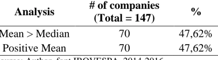
Table 3 - Exporters – Descriptive Statistics

(Total = 147) %

The table above shows that we have 70 companies with an average value greater than the median, an increase of 9 companies when we compare to the period before crisis.

As Brazil is living in a lasting economic crisis, the value of the dollar has helped those who export. With the real depreciated against the dollar, the product/service costs even less abroad. Let's look at the chart below: IBOVESPA X BRL/USD:

Graph 8 – IBOVESPA X BRL/USD

Source: MORTOZA & PIQUEIRA, 2017 Graph IBOVESPA X BRL/USD

(31)

distanced itself from the exchange rate. In this period, the dollar closed at R$ 2.65, reaching a 13% increase. Just in December, the increase was 8.61%.

As we did before, let's understand the Std.Deviation values for the top 4 companies, in terms of values.

MNPR3 – Minupar – Mngt.

LUPA3 – Lupatech – Equipments and Services for Oil and Gas NORD3 – Nordon – Metalurgy

TOYB3 – TecToy - Eletronics

As we can see above, the graphs present a certain similarity to the period before the crisis, but for non-exporters. Demonstrating a degree of uncertainty on the part of investors.

For LUPA3, an oil and gas company, the crisis was accompanied by a judicial recovery process. This process is due to the crisis of one of its biggest clients, Petrobras and also under

650 585 520 455 390 325 260 195 130 65 1 500 400 300 200 100 0 Data Points M N P R 3

Time Series Plot of MNPR3

650 585 520 455 390 325 260 195 130 65 1 700 600 500 400 300 200 100 0 -100 -200 Data Points LU P A 3

Time Series Plot of LUPA3

650 585 520 455 390 325 260 195 130 65 1 30 20 10 0 -10 -20 Data Points N O R D 3

Time Series Plot of NORD3

650 585 520 455 390 325 260 195 130 65 1 1500 1000 500 0 -500 -1000 Data Points T O Y B 3

(32)

the drastic reduction of the price of a barrel of oil in the international market. In this way, the market reacted with an increase in the perception of risk, keeping the data dispersion more homogeneous.

As the graphs plotted above presented a different behavior of the period before the crisis, for the companies with higher Std. Deviation, we will now analyze the companies with less variation.

COCA34 – Coca Cola – Beverage COLG34 – Colgate – Healthcare

PGCO34 – Procter & Gamble – Food and Healthcare RANI3 – Celulose Irani – Celullose

Graph 10 - Times Series – Returns – Lower Std.Deviation

As can be seen, the graphs show a similar behavior in comparison with each other. PGCO34 - Investment of R $ 280 million in a new plant in Brazil in the years 2014/2015.

650 585 520 455 390 325 260 195 130 65 1 7,5 5,0 2,5 0,0 -2,5 -5,0 Data Points C O C A 3 4

Time Series Plot of COCA34

650 585 520 455 390 325 260 195 130 65 1 10 5 0 -5 -10 Data Points C O LG 3 4

Time Series Plot of COLG34

650 585 520 455 390 325 260 195 130 65 1 8 6 4 2 0 -2 -4 -6 -8 Data Points P G C O 3 4

Time Series Plot of PGCO34

650 585 520 455 390 325 260 195 130 65 1 10 5 0 -5 -10 Data Points R A N I3

(33)

The COCA34 had one of the worst moments since 1930, reaching 3% negative in 2015. COLG34, in the second quarter of 2015, saw a drop of $ 48 million compared to the same period last year.

In turn, RANI3 presented a 18.1% higher margin than in 2015.

This shows us that even during all the challenges encountered in the economic environment during the year 2015, it is possible to grow.

4.2.2 Non Exporters

For a company to become global, it must go through eight stages: export, installation of a representation, commercial distribution, opening a sales subsidiary, joint manufacturing, local manufacturing with own resources, multinationalisation of companies, globalization of the company (NOSÉ JUNIOR, 2005).

However, in this path, there are several internal challenges, since companies have a lack of knowledge and understanding of the incentives offered by the federal government. This leaves a gap for further development. It is also noted that the domestic market often does not have the productive capacity to increase a larger volume of exports, since the products to be exported are specific to a certain segment (niche).

As a starting point, a descriptive statistics is shown below:

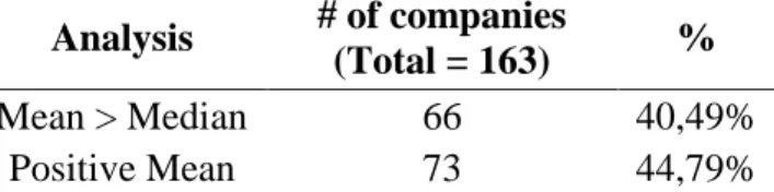
Table 4: Non Exporters – Descriptive Statistics

(Total = 163) %

Compared to the previous period, there was an increase of 5 companies with the average higher than the median, rising from 37.2% to 40.49%. This factor can be explained by the uncertainty perceived by investors. For a better evaluation, we now analyze the 4 companies with the highest Standard Deviation to understand a possible change over the previous period already presented.

They are:

VIVR3 – Viver Construtora – Construction PDGR3 – PDG – Real State

(34)

TCNO4 – Tecnosolo – Engineering CTAX3 – Contax – Third party services

The companies represented above have a profile very close to that presented previously for the same group, non exporters. The low dispersion of data shows that risks can be reduced as they are constant.

VIVR3, the top left graph was also shown as one with the higher Std. Deviation among the population, before crisis.

The next analysis will be done for companies that presented the lowest Std. Deviation among the population of 163.

They are:

CALI4 – Construtora Adolpho Lindenberg – Construction Company LIPR3 – Eletrobras – Energy

CEEB3 – Companhia de Eletricidade do Estado da Bahia – Energy BUET3 – Construtora Lix da Cunha – Buildings

650 585 520 455 390 325 260 195 130 65 1 500 400 300 200 100 0 Data Points V IV R 3

Time Series Plot of VIVR3

650 585 520 455 390 325 260 195 130 65 1 400 300 200 100 0 Data Points P D G R 3

Time Series Plot of PDGR3

650 585 520 455 390 325 260 195 130 65 1 300 200 100 0 -100 -200 -300 Data Points T C N O 4

Time Series Plot of TCNO4

650 585 520 455 390 325 260 195 130 65 1 500 400 300 200 100 0 Data Points C T A X 3

(35)

Graph 12 – Times Series – Returns – Lower Std.Deviation

In all the above graphs, it is possible to notice a very small or almost zero dispersion for the period from 2014 to 2016. Except for CEEB3 and LIPR3, which, due to the transfer of costs by the government, assumed an increase of 11.43 % on light beads.

279 248 217 186 155 124 93 62 31 1 0,50 0,25 0,00 -0,25 -0,50 Data Points C A L I4

Time Series Plot of CALI4

650 585 520 455 390 325 260 195 130 65 1 4 3 2 1 0 -1 -2 -3 -4 -5 Data Points L IP R 3

Time Series Plot of LIPR3

650 585 520 455 390 325 260 195 130 65 1 7,5 5,0 2,5 0,0 -2,5 -5,0 Data Points C E E B 3

Time Series Plot of CEEB3

650 585 520 455 390 325 260 195 130 65 1 0,50 0,25 0,00 -0,25 -0,50 Data Ponits B U E T 3

(36)

5 COMPARATIVE ANALYSIS

Now that we have understood of how each group of companies behaved, we need to comparatively analyze the 2 periods involved. In this way, we will be able to punctuate and validate their relationship, statistically and economically.

To do this, we will start by compile all data points involved, separating them into Before the Crisis and During the Crisis. See table 5 below:

Table 5 – Descriptive Statistics for Before X During Crisis

As we can see in the table, the data behave very differently in the two periods.

The mean value for the period before the crisis is negative and the average during the crisis is positive. This is 0 for non-exporting companies during the crisis. This means that during the crisis, the companies that exported, obtained (on average) a greater daily return in relation to the companies that did not export.

The standard deviation is also quite different in the two periods, with the pre-crisis period showing up to 50% greater than the period during the crisis. Denoting that the dispersion was smaller, but with significant difference between them.

And if we look at kurtosis, we can observe a significant increase, positively. This positive value indicates that the distribution has heavier tails and a more pronounced peak than a normal curve, in other words, daily returns have focused more to the center of the curve.

However, we need to check if the difference is statistically significant between the companies and the periods before and after the crisis. To make it, let's start with the 2 variance

comparison test.

To start is needed to set a Null and an Alternative hypothesis such as:

NULL =>H0: σ²1 / σ²2 = K

The ratio between the first population standard deviation (σ²1) and the second population standard deviation (σ2) is equal to the hypothesized ratio (K).

ALTERNATIVE => H1: σ²1 / σ²2 ≠ K

The ratio between the first population standard deviation (σ²1) and the second population N Total Mean Std. Deviation Median Kurtosis N Total Mean Std. Deviation Median Kurtosis Exporters 92398 -0,06 20,00 0,00 211,40 91354 0,05 9,96 0,00 5373,62 Non Exporters 105607 -0,04 11,89 0,00 476,73 100645 0,00 5,97 0,00 2612,66 During Crisis (Jan/2014 to Jun/2016) Before Crisis (Jan/2011 to Dec/2013)

(37)

standard deviation (σ²2) does not equal the hypothesized ratio (K). In our case, as we test the equality, K=1.

Figure 3 – 2 variance comparison test – Exporters: Before X During Crisis

Ratio of Standard Deviations

Estimated Ratio 95% CI for Ratio using Bonett 95% CI for Ratio using Levene 2,00714 (1,646; 2,736) (*; *) Test Null hypothesis H₀: σ²₁ / σ²₂ = 1 Alternative hypothesis H₁: σ²₁ / σ²₂ ≠ 1 Significance level α = 0,05 Method Test Statistic DF1 DF2 P-Value Bonett * 0,000 Levene 253,91 1 183692 0,000 Source: Author

As the p-value (0.000) is lower than the significance level that we consider by default (0.05), we reject the null. Thus, the statistical evidence of the sample points for the difference between the variances. Thus, the variance decreases during the crisis and the difference is statistically significant. So, we can conclude that the risk in these stocks during the crisis has been smaller.

Now we are going to test the variance and standard deviation of companies that are non exporters.

Figure 4 – 2 variance comparison test – Non Exporters: Before X During Crisis

Ratio of Standard Deviations

Estimated Ratio 95% CI for Ratio using Bonett 95% CI for Ratio using

(38)

Levene 1,99175 (1,711; 2,415) (*; *) Test Null hypothesis H₀: σ²₁ / σ²₂ = 1 Alternative hypothesis H₁: σ²₁ / σ²₂ ≠ 1 Significance level α = 0,05 Method Test Statistic DF1 DF2 P-Value Bonett * 0,000 Levene 54,22 1 205491 0,000 Source: Author

As the P-value ≤ α, we must reject H0 and assume that the standard deviation or variance is statistically significant. In other words, the period before and after crisis for non exporters are also different.

To continue with our analysis, the next step will be the 2 sample t-test, a comparative test for means.

For exporters, the analysis is as follows:

Figure 5 – 2 sample t test – Exporters: Before X During Crisis

Method

μ₁: mean of ALL_Exporters_Before µ₂: mean of ALL_Exporters_During Difference: μ₁ - µ₂

Equal variances are not assumed for this analysis.

Test Null hypothesis H₀: μ₁ - µ₂ = 0 Alternative hypothesis H₁: μ₁ - µ₂ ≠ 0 T-Value DF P-Value -1,54 135844 0,124 Source: Author

As the P-value ≥ α, we must accept H0 and assume that the means are not statistically different. In other words, the average rate of returns, before and after the crisis, is not different.

As we did for exporting companies, we now need to test the means of non-exporting companies.

(39)

Figure 6 – 2 sample t test – Non Exporters: Before X During Crisis

Method

μ₁: mean of ALL_Non Exporters_Before µ₂: mean of ALL_Non Exporters_During Difference: μ₁ - µ₂

Test Null hypothesis H₀: μ₁ - µ₂ = 0 Alternative hypothesis H₁: μ₁ - µ₂ ≠ 0 T-Value DF P-Value -1,02 157216 0,306 Source: Author

The same result of the comparison between exporting companies, the average return is not statistically different between the two periods as we don´t reject the null hypothesis where we state the equality of the means.

And as a final test, we need to understand whether exporting companies stand out from non-exporters as a whole.

That said; let's start with the 2 variance comparison test.

Figure 7 – 2 variance comparison test – Exporters X Non Exporters: 2011 to 2016

Test Null hypothesis H₀: σ²₁ / σ²₂ = 1 Alternative hypothesis H₁: σ²₁ / σ²₂ ≠ 1 Significance level α = 0,05 Method Test Statistic DF1 DF2 P-Value Bonett * 0,000 Levene 252,75 1 389185 0,000 Source: Author

Since the P-value ≤ α, let us reject H0 and assume that the variances are statistically different.

To continue and complete the tests, let's understand the mean variance of each group of companies and prove whether or not they are divergent by using the 2 sample t test.

(40)

Method

μ₁: mean of Exporters µ₂: mean of Non Exporters Difference: μ₁ - µ₂

Test Null hypothesis H₀: μ₁ - µ₂ = 0 Alternative hypothesis H₁: μ₁ - µ₂ ≠ 0 T-Value DF P-Value 0,41 293495 0,685 Source: Author

And as a result, we need to accept the null hypothesis, since the p-value found is 0.685. This shows that when we speak of a group of companies, exporting or not exporting, they do not differentiate in a period of crisis, since the variation ends up being absorbed.

Based on all results, we conclude that the variance of returns for exporters has reduced after crisis and the difference is statistically significant. This means that the risk of this kind of stocks decreases with the crisis. In term of the means of returns the difference is not statistically significant. Thus, even if there is an increase, the difference didn´t become statistically significant.

(41)

6 CONCLUSIONS

The indicator of whether or not a country is in crisis is the strong economic recession, and in this case, there has been a decline in the Gross Domestic Product (GDP) since 2014, where it remained negative for two consecutive years, 2015 and 2016. In 2013, what has been called a "chicken flight" happened, an expression that is used by economists to characterize the swings in a country's growth. Usually we say that some indicator behaves like chicken flight when it increases for a short period, 1 to 2 years and then remains without or with absence of expansion of economic activity.

In the course of the study, we could see that the distribution of shares of exporting companies did not follow the same profile of non-exporting companies, regardless of whether before or after the crisis of 2014. This analysis was based on IBOVESPA daily returns.

The Bovespa Stock Index decreased more than 20% so far this year, making it the worst performer among the major emerging markets (ROONEY, 2013)

Brazil has been alternating short cycles of economical phases, since the end of dictatorship regime in 1985, with macroeconomics oscillating. During 2011, a year characterized by optimism from Labor Party, started to show up signals for a crisis. From 2014 on, many corruption scandals erupted (MORTOZA & PIQUEIRA, 2017).

In this study, we were able to prove that the companies that were allocated as Exporters presented the same mean variation. However, their dispersion of daily returns is proven to be different in a separate period (Before and During). The higher the variance, the farther from the mean the values will be, and the lower the variance, the closer the values will be to the mean. In other words, they were more risky for investors, but the one who invested in exporting companies,had their earnings insured.

With this affirmation above, we can answer the hypothesis raised in this work: “Are the

returns from Brazilian companies that export and those who do not export economically/statistically significant during and after the crisis period?”

Yes, there is a significant difference for the companies who export during the crisis, presenting a higher standard deviation/variance in comparison with the non exporting companies.

The companies have a statistically proven difference, since the test 2 sample t test presented 0.000 as a p-value as a result for companies that export in the periods before and after the crisis.

(42)

Said that, the best and most profitable strategy for companies is undoubtedly export. Since they use the volume and prices of exported products to make it possible to soften the inconstancies in Brazilian market. In this paper, we have effectively analyzed 147 companies that were more profitable economically compared to the 163 that did not export. In this way, we can say that exporting to a Brazilian company is something to be pursued.

(43)

7 BIBLIOGRAPHY

ARAÚJO, Bruno César Pino Oliveira de; & PIANTO, Donald Matthew. (2010). Export

potential of Brazilian industrial firms. Economia Aplicada, 14(4), 277-297.

ABEL, Andrew. (1988). Stock prices under time-varying dividend risk: An exact solution in

an infinite- horizon general equilibrium model. Journal of Monetary Economics 22, 375-393.

AMADEO, Kimberly. (2017). What are Interest Rates? How do they work?. Acess on: <https://www.thebalance.com/what-are-interest-rates-and-how-do-they-work-3305855>. June.

AW, B. Y. & HWANG, A. R. (1995). Productivity and the export market: A firm-level

analysis. Journal of Development Economics 47, 313–332.

ALVAREZ, Roberto; LOPEZ, Ricardo A. (2005). Exporting and performance: evidence from

Chilean plants. Canadian Journal of Economics.

BINDER, J. J.; MERGES, M.J. (2001). Stock Market Volatility and Economic Factors [Online] Available at: <http://papers.ssrn.com/sol3/papers.cfm?abstract_id=265272>. [Accessed 9 November 2016].

BLACK, Fischer. (1976). Studies of stock price volatility changes. In: Proceedings of the 1976 Meetings of the Business and Economics Statistics Section. American Statistical Association, 177-181.

BLOOMBERG, L.P. (2015). Brazil´s political Crisis puts the entire economy on hold [Online] Available at: <https://www.bloomberg.com/news/articles/2015-08-18/from-planes-to-cafes-brazil-s- economy-on-hold-as-crisis-deepens>. [Accessed 9 November 2016].

BRIGUGLIO, L.; CORDINA, G.; FARRUGIA, N., and VELLA, S. (2009). Economic

Vulnerability and Resilience: Concepts and Measurements. Oxford Development Studies, Vol.

37, No. 3, pp. 229–247.

BASILE, Roberto. (2001). Export behaviour of Italian manufacturing firms over the nineties:

the role of innovation. Research Policy 30 (2001) 1185–1201.

BLECKER, Robert A. (2010). Open economy models of distribution and growth. Working Papers 2010-3. American University, Department of Economics.

BEKAERT, Geert and HARVEY, Campbell R. Capital flows and the behavior of emerging market equity returns. National Bureau of Economic Research. Working paper No. 6669. 1998

BERNARD, A. B. and JENSEN, J. B. (1995). “Exporters, Jobs, and Wages in the U.S.

Manufacturing: 1976-1987”. Brookings Papers on Economic Activity, pp. 67-119.

BERNARD, Andrew B; JENSEN, J. Bradford. (1999) Exceptional exporter performance:

cause, effect, or both?. Journal of International Economics. Volume 47, Issue 1, 1 February,

Pages 1-25.

BERNARD, Andrew B.; & JESEN, J. Bradford. (2004). Exporting and Productivity in the