Assessing finantial distress through finantial ratios

(1)

I N S T I T U T O P O L I T É C N I C O D E L I S B O A

I N S T I T U T O S U P E R I O R D E C O N T A B I L I D A D E

E A D M I N I S T R A Ç Ã O D E L I S B O A

A S S E S S I N G F I N A N C I A L D I S T R E S S

T H R O U G H F I N A N C I A L R AT I O S

Bruno Fernando Lima Reis

(2)

(3)

iii I N S T I T U T O P O L I T É C N I C O D E L I S B O A I N S T I T U T O S U P E R I O R D E C O N T A B I L I D A D E E A D M I N I S T R A Ç Ã O D E L I S B O A

A S S E S S I N G F I N A N C I A L D I S T R E S S

T H R O U G H F I N A N C I A L R AT I O S

Bruno Fernando Lima Reis

Dissertação submetida ao Instituto Superior de Contabilidade e Administração de Lisboa para cumprimento dos requisitos necessários à obtenção do grau de Mestre em Análise Financeira, realizada sob a orientação científica do Professor Doutor Joaquim António Martins Ferrão.

Constituição do Júri:

Presidente - Prof. Especialista José Nuno Teixeira de Abreu de Albuquerque Sacadura Arguente - Prof. Especialista Mário Nuno Neves da Silva Mata

Vogal - Prof. Doutor Joaquim António Martins Ferrão

(4)

I declare to be the author of this dissertation, which constitutes an original and unpublished work, which has never been submitted (in its entirety or any of its parts), to another higher education institution to obtain an academic degree or other qualification. I also certify that all quotations are duly identified. Moreover, I am aware that plagiarism - the use of extraneous elements without reference to its author - constitutes a serious lack of ethics, which may result in the annulment of this dissertation.

(5)

v

“But the age of chivalry is gone.

That of sophisters, economists, and

calculators, has succeeded; and the

glory of Europe is extinguished

forever.”

(6)

Acknowledgement

I would like to thank my dissertation advisor Professor Doutor Joaquim Ferrão at Instituto Superior de Contabilidade e Administração de Lisboa. His office door was always open whenever I had a question about my research or writing. He consistently allowed this paper to be my own work, but steered me in the right the direction whenever he thought I needed it.

I would like also to thank my father Fernando Reis for his constant incentive and for his words of support.

(7)

vii

Abstract

This study aims to investigate if an early warning model for the financial distress can be applied to Portuguese companies for the manufacturing industry, and which variables are the most relevant. The early prediction of financial distress can be of capital importance to warn the relevant parties so they can act and take all the necessary actions in an early stage of financial difficulties.

As financial distress is often associated with corporate bankruptcy, by preceding it, in this dissertation we have also intended to distinguish between these two concepts. According to some authors, financial distress and corporate bankruptcy are not part of the same process; they are actually two different processes.

(8)

List of Tables

Table 2.2.1.1 - Relative Contribution of the Variables ... 10

Table 2.2.1.2 - Results one year prior to bankruptcy ... 11

Table 2.2.1.3 - Results two years prior to bankruptcy ... 11

Table 2.2.1.4 - Bankruptcy thresholds (Z-Score and Z’-Score) ... 13

Table 2.2.1.5 - Bankruptcy thresholds (Z-Score, Z’-Score and Z’’-Score) ... 13

Table 2.3.1 - Variables in the Final Early Warning Model (2002) ... 22

Table 3.3.1 - Variables Correlation ... 31

Table 3.3.2 - Sample Characteristics ... 32

Table 3.3.3 - Summary of firms in financial distress ... 33

(11)

xi

List of Figures

(12)

List of Abbreviations

AMEX - American Stock Exchange BSM - Black–Scholes–Merton CA - Current Assets

CAPEX - Capital Expenditure CF - Cash Flow

CL - Current Liabilities

CLTD - Current portion of long-term debt EBIT - Earnings Before Interest and Tax

EBITDA - Earnings Before Interest, Tax, Depreciation and Amortization FD - Financial Distress

FINL - Financial Leverage GDP - Gross Domestic Product INE - Instituto Nacional de Estatística LIQ - Liquidity

MDA - Multivariate Discriminate Analysis NP - Notes Payable

NYSE - New York Stock Exchange POP - Population

QR - Quick Ratio ROA - Return on Assets SA - Sociedade Anónima

SABI - Sistema de Análisis de Balances Ibéricos SAMP - Sample

(13)

xiii TA - Total Assets

TD - Total Debt

TIE - Times Interest Earned UK - United Kingdom US - United States WC - Working Capital

(14)

1. Introduction

Since Beaver (1966) understanding the motives behind corporate bankruptcy has been of significant importance amongst academics and experts.

Bankruptcy has a negative impact on the entire company and on all the involved stakeholders: managers, employees, customers, suppliers, financial institutions.

According to Platt and Platt (2006), bankruptcy and financial distress are not two sequential steps. Firms experience financial distress after poor operating results or due to external factors. On the other hand, bankruptcy is an action firms take to protect their assets from creditors.

An early prediction of firm’s financial distress can help banks and private investors to take defensive measures before a financial collapse.

Following the research of Platt and Platt (2006 and 2008), our aim is to evaluate if an early warning model for the financial distress can be applied to Portuguese companies from the manufacturing industry.

As corporate bankruptcy and financial distress are often associated, on chapter 2 we went through the main literature (and prediction models) on both concepts, hoping to provide some clarity on their differences and similarities.

On chapter 3 we have explained the methodology applied. We have used a logit regression and used a similar financial distress criterion as Platt and Platt (2006 and 2008). For the choice of the independent variables, we have used five variables that were present in the global financial distress prediction model of Platt and Platt (2008) and we have included seven additional independent variables.

As for the sample selection, we have decided to analyse Portuguese companies only from the manufacturing industry, whose legal form was public limited company and limited liability company (corresponding to “Sociedade Anónima” and “Sociedade Limitada” in the Portuguese legal context, respectively) and with sales above EUR 2.5 million for the years 2006 to 2017. The restriction to the manufacturing industry is based on the fact that we use financial data where the lack of homogeneity in different sectors leads to considerable distortions in the results.

(15)

2  The agency conflicts are evident in the three periods analysed, as firms which legal form is “Sociedade Anónima” are more susceptible to enter into financial distress;

 Market diversification (measured through the level of exportation in total sales) reduces the likelihood of firms entering into financial distress;

 Sales growth in difficult times (crisis) is also an important signal in the reduction of the probability of financial distress;

 Age seems to behave as in living beings, the older the firm the greater the probability of disappearing;

 Assets profitability (measured through EBITDA to Total Assets) is always statistically significant and always with a very significant coefficient.

(16)

2. Theoretical Framework

2.1 Bankruptcy

The bankruptcy of a company represents an event that is associated with negative feelings, at great losses for all stakeholders.

The bankruptcy phenomenon is not restricted to a single sector or product; it is transversal to all areas. Bankruptcy is closely related to liquidity problems and it is at this point that the warning signal is often issued for a possible situation of bankruptcy (Famá & Grava, 2000). According to Sharma and Mahajan (1980), ineffective management and unforeseen events are the two main causes that lead a company to bankruptcy. Santos (2000) also verified that the two main causes that lead a company from a "healthy" to an "unhealthy" situation are the management’s ineffectiveness and a deficient financial structure.

Notwithstanding, there are several causes or factors that can lead a company to bankruptcy, which the literature generally classifies as external and internal factors. Jacobsen and Kloster (2005), through a study in Norway focusing on the macroeconomic (external) factors present during a bankruptcy process, concluded that changes in profit margins, competitiveness, real interest rates, as well as constant cyclical fluctuations, are the ones that have contributed the most to a rise in bankruptcies in recent years.

Campbell and Underdown (1991) say that in most cases, bankruptcy is the result of a set of factors that lead a company to failure, and it cannot be affirmed with absolute certainty that it was only because of a particular factor. According to these authors, external changes and poor internal management lead to serious imbalances in the firm's operational performance, resulting in bankruptcy.

Regarding the issue of ineffective management, Laia (1999) explains that it is not always easy to evaluate whether a particular management board of a company is acting correctly or not. Nevertheless, Laia (1999) says that, ultimately, it is the management board that carries the responsibility of monitoring the company’s progress. If the management board is really effective it would be able to monitor the external environment in order to prevent more intricate situations.

(17)

4 Laia (1999) recognized two types of bankruptcy causes: strategic/economic and financial. In relation to the strategic/economic causes, the author considered the economic recession, punctual bad business, ineffective management, the lack of competitiveness and markets, and an inadequate strategy to be the most relevant causes. In relation to the financial causes, the author considered the rise in the interest rates, the poorly negotiated financing and the capital structure to be the most significant causes.

Bescos (1987) described some of the first causes that lead a company to failure, being: activity reduction (33,2%), management difficulties (23%), treasury problems (18,7%), margins and profitability reduction (17,6%) and accidental causes (7,5%), indicating this way that the causes of potential bankruptcies are mostly internal.

Brilman (1993), like Laia (1999), argues that managers are the main culprits. Mader’s (1977) study shows that most companies had known their financial difficulties for 3 to 5 years, but they still continued recruiting and investing some months before bankruptcy. Brilman (1993) points out some of the explanations that are intertwined with managers' late reaction, such as the expectations that the situation will improve, the use of outdated indicators, over-optimistic budgets, the use of easy solutions, and the management incapability in the face of crisis, among others. Therefore, reacting late can cause huge losses for companies, where at some point there is no "cure" that can save a company.

Beaver (1966) considers the company’s solvency as a "reservoir" of funds, which is supported by inflows, from where the company fulfils its obligations, that is, outflows. However, when this "reservoir" at one point is exhausted, the company tends to default on its obligations, that is, it tends to bankruptcy; whereas Altman (1968) and Deakin (1972) consider the concept of bankruptcy at a juridical level.

Blum (1974) adopts as concept of bankruptcy the inability of a company to pay its debts and thus enter into an agreement to reduce debts or enter into insolvency proceedings. On the other hand, Ohlson’s (1980) study considers as bankrupt a company that has filed for insolvency or has been declared insolvent.

Taffler (1982) defines bankruptcy as a voluntary liquidation or court order, while Karels and Prakash (1987) consider that the exact moment when a company's bankruptcy occurs is difficult to identify and therefore to these authors bankruptcy is a process that initiates when the financial difficulties arise and ends when the situation is legally concluded.

(18)

According to Santos (2000), bankruptcy can be defined as the economic-legal condition of the company that makes it impossible to meet its commitments, resulting in "legal bankruptcy", that is, bankruptcy decreed in court.

In the third edition of their book “Corporate Financial Distress and Bankruptcy”, Altman and Hotchkiss (2006) seek to clarify different generic terms that are frequently used in the literature: failure, insolvency, default and bankruptcy.

Regarding failure, the authors divide it in two different criteria: economic failure when the rate of return on an investment is lower than the rates of return on similar investments; and legal failure when the firm is not able anymore to respect the legally enforceable demands of its creditors. The term legal may or may not involve a court order.

According to Altman and Hotchkiss (2006), insolvency is related to a negative performance of a firm and it takes place when a firm is not able to meet its current obligations on the back of a shortage of liquidity, to what the authors call technical insolvency. The authors also mention “insolvency in a bankruptcy sense” which is more related to a chronic rather than to a temporary situation. This situation occurs when the fair value of a firm’s total assets is exceeded by total liabilities, with the firm’s equity being negative. Lastly, the authors add the concept of “deepening insolvency”, which is used when an eventually bankrupt firm is supposed to be maintained in existence needlessly and to the disadvantage of the estate, particularly the creditors.

In turn, the term default essentially reflects the relationship between the firm and its creditors. The authors consider two types of default: technical and legal. Technical default occurs when the firm does not respect a certain contractual agreement towards its creditor (e.g., the breach of a financial covenant), which can be used for a legal proceeding, resulting in legal default.

Lastly, as for bankruptcy, the authors mention two types of bankruptcy: when a firm reaches a situation of negative equity; and when a formal declaration of bankruptcy is requested in court, including a request either to liquidate the firm’s assets or attempt a recovery program, legally referred to as bankruptcy reorganisation.

During the last decades different concepts such as bankruptcy, insolvency, suspension of payments, voluntary liquidation, and others were used. The definition of a universal concept is therefore not easy, and in fact it is a limitation, since the selection of the sample of companies or entities depends on the clarity of this concept.

(19)

6

2.2 Bankruptcy Prediction Models

It comes to light the need to gather a set of information that predicts and anticipates situations of bankruptcy, the credit scores. They are increasingly useful in investment decision making, credit and business diagnosis. The models use statistical techniques, which select indicators that combined give a clear classification if the company belongs to a group in risk of bankruptcy, or on the contrary is in a favourable situation. These indicators can anticipate financial distress situations, giving managers time to try to circumvent the problem and improve the company's performance.

The source of the ratios are the financial statements, in particular the balance sheet and the income statement. The balance sheet reflects the company's financial position on a given date. The income statement shows the company's financial performance in the period. As for the evolution of corporate credit scoring models, Altman and Hotchkiss (2006:234) have made the following compilation:

 Qualitative (Subjective models);

 Univariate (use of ratios based on accounting or market indicators for risk assessment);  Multivariate (including Discriminant, Logit, Probit, Nonlinear Models and Neural Networks);

 Discriminant and Logit Models in Use (including consumer models, Z-Score, ZETA Score, Private Firms Models (e.g., Z’’-Score));

 Artificial Intelligence Systems (Expert Systems, Neural Networks (e.g., Standard & Poor’s Credit Model);

 Option/Contingent Claims Models;

 Blended Ratio/Market Value Models (including Moody’s Risk Calculation, Z-Score (Market Value Model)).

The statistical techniques most widely used in credit scoring are parametric models and non-parametric models. Within the non-parametric models there are univariate analyses and multivariate analyses; discriminant analysis, logit and probit are inserted into the latter group. The discriminant analysis intends to discriminate risk groups by analysing a set of characteristics, assigning a score to each independent variable resulting from a weighted average of values.

(20)

The logit and probit models are based on a logistic function and on a normal function working similarly to a linear regression model that starts from subpopulations to discriminate risk groups. The calculation of the logistic coefficients compares the probability that an event will happen with the probability that it will not happen.

Ferrando and Blanco (1998) also consider that, like the discriminant analysis, the logit model presents as disadvantage the error margins; it has as main advantage the fact that in addition to allowing the use of financial ratios as independent variables, it also allows non-financial or qualitative information.

Wu, Gaunt and Gray (2010) made a comparison of alternative bankruptcy prediction models. On their study, the authors tested five major bankruptcy prediction models:

 Altman (1968) – MDA model based on accounting variables;  Ohlson (1980) – logit model with accounting ratios;

 Zmijewski (1984) – probit model using accounting data;

 Shumway (2001) – hazard model with both accounting and market variables; and  Hillegeist et al. (2004) – BSM-Prob model based on both accounting and market

variables.

Wu et al. (2010) have also developed a new model containing key variables from each of the above mentioned five models and added a new variable that proxies for the degree of diversification within the firm. This new variable showed to be negatively associated with the risk of bankruptcy.

On their study, Wu et al. (2010) say that each model captures to some extent different characteristics of corporate financial health and that a combined model is more likely to offer more consistent and more reliable results. According to the authors, each model uses a set of different independent variables (accounting, market and firm-specific data and implicit probabilities from option-pricing models) and a variety of different econometric conditions (multiple discriminant analysis, logit, probit, and hazard models).

The authors conclude that the most relevant accounting information relates to profitability, liquidity and leverage. In particular, bankruptcy is more likely for firms with:

 Relatively lower earnings before interest and tax (EBIT) to total assets;  A higher decrease in net income;

(21)

8  A comparatively low working capital to total assets; or

 A high market-based leverage (total liabilities to the market value of total assets). As for the results of the comparison of the different bankruptcy prediction models Wu et al. (2010) conclude that:

 The Altman (1968) MDA model shows a poorer performance in comparison to other models in the literature;

 The accounting-based models of Ohlson (1980) and Zmijewski (1984) show an adequate performance during the 1970, but it has deteriorated over more recent periods;

 Shumway (2001) hazard model, which includes market data and firm-characteristics, in general shows a better performance than the accounting-based models;

 Hillegeist et al. (2004) market-based probability of bankruptcy based on the Black– Scholes–Merton option-pricing model presents a satisfactory performance but is generally inferior to the Shumway (2001) model.

All the five corporate bankruptcy prediction models mentioned above will be further detailed in the following pages.

2.2.1 Altman ’s Mul tivari ate Discri min ate An alysis (MDA)

2.2.1.1 Altman’s Z-Score (1968) model

This model was developed by Altman (1968) and is currently one of the most important models, known and used, that combines different measures of profitability and risk. This model has proven to have a good bankruptcy predictive capacity in diverse contexts and markets.

Altman (1968) used a sample of 66 market listed industrial companies, of which 33 belonging to group 1 (bankrupt) and the other 33 to group 2 (non-bankrupt) for the period 1946 to 1965. Data was extracted from the financial statements previous to bankruptcy and the variables were classified into 5 categories: liquidity, profitability, leverage, solvency and activity ratios.

In his study, Altman (1968) selected only five ratios: X1 =

Working capital Total Assets

(22)

According to Altman (1968) this ratio is a measure of net liquid assets of a company in relation to the total assets. Working capital is defined as the difference between current assets and current liabilities. Altman (1968) also refers that a company that is constantly having operating losses will see its current assets consumed in relation to total assets.

X2 = Retained earnings Total Assets

Retained earnings is an indicator that reflects the accumulation of profits. For Altman (1968), this indicator underlies the age of the company, i.e. a more recent company will initially have lower accumulated profits in comparison to an older company. This suggests that younger companies may be discriminated, but Altman (1968) refers that in the real world the chances of bankruptcy are higher in the first years of activity of a company.

X3 = EBIT Total Assets

EBIT stands for earnings before interest and tax reductions. According to Altman (1968) it is a measure of the true productivity of the company’s assets as it excludes tax or leverage factors. Altman (1968) also refers that this ratio is of particular interest for studies of corporate failure as ultimately the existence of company is based on the earning power of its assets.

X4 = Market value equity Book value of total debt

According to Altman (1968) the market value of equity represents the market capitalization and debt includes both current and long-term. It is a measure of how much the assets can drop in value before the liabilities exceed the assets and the company becomes insolvent.

X5 = Sales Total Assets

Lastly, we have the ratio that shows the company's ability to generate sales based on its assets. According to Altman (1968) this ratio is quite important as it is the least significant ratio on an individual basis. Altman (1968) mentions that this ratio is not statistically significant but due to a unique relationship to other variables in the model, this ratio is of high importance for the contribution to the discriminating ability of the model.

(23)

10 Altman (1968) observed that the variables X1, X2, X3 and X4 are all significant at the 0.001 level, showing notable differences between the two groups. Variable X5 was the only one that did not show a noteworthy disparity between the two groups.

However, Altman (1968) sought to evaluate the relative explanatory contribution of each variable in relation to the total discriminatory power of the function and the interaction between them. As the variable measurement units are not all comparable to each other, the coefficients were adjusted. Table 2.2.1.1 shows the variables ranked according to their relative contribution to the discriminatory power of the function:

Table 2.2.1.1 - Relative Contribution of the Variables

Variable Scaled Vector Ranking X1 3.29 5 X2 6.04 4 X3 9.89 1 X4 7.42 3 X5 8.41 2

Source: Adapted from Altman (1968)

Altman (1968) thus concludes that, the variables X3, X5 and X4 are the ones that contribute the most to discriminate the different groups of companies. Therefore, according to the original study of Altman (1968), the discriminant function for listed companies is as follows:

Z = 0,012X1 + 0,014X2 + 0,033X3 + 0,006X4 + 0,999X5 (2.2.1.1)

Altman (1968) refers that all firms with a Z-Score higher than 2,99 fall into the “non-bankrupt” group, while the firms with a Z-Score below 1,81 are bankrupt. To the author all the companies presenting a Z-Score between 1,81 and 2,99 are considered to be in a “zone of ignorance” or “grey area”.

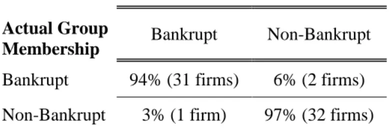
In Table 2.2.1.2, we have the results of Altman's (1968) study for one year before bankruptcy, which revealed the following:

(24)

Table 2.2.1.2 - Results one year prior to bankruptcy Predicted

Actual Group

Membership Bankrupt Non-Bankrupt

Bankrupt 94% (31 firms) 6% (2 firms) Non-Bankrupt 3% (1 firm) 97% (32 firms)

The model had a type I error of 6% indicating that the model for one year prior to bankruptcy classified 2 out of 33 bankrupt firms as non-bankrupt. On the other hand, it obtained a type II error of 3%, that is, of the 33 non-bankrupt firms, the model classified one as bankrupt, thus showing that the model obtained a predictive capacity of 95% for one year prior to bankruptcy.

Finally, the results of Altman's (1968) study for two years before bankruptcy revealed the following:

Table 2.2.1.3 - Results two years prior to bankruptcy Predicted

Actual Group

Membership Bankrupt Non-Bankrupt

Bankrupt 72% (23 firms) 28% (9 firms) Non-Bankrupt 6% (2 firms) 94% (31 firms)

As shown in Table 2.2.1.3, for two years prior to bankruptcy, type I and II errors were 28% and 6%, respectively, thus indicating that the Z-Score model reached an accuracy of 83%. Altman (1968) tested the model up to five years before bankruptcy, showing that as the number of years increase, the model's accuracy decline.

It should be noted that Altman's Z-Score model (1968) has its limitations, such as the fact that qualitative data cannot be included, that is, the financial data considered do not reflect unforeseen events that may occur in the firm's activity and which are sometimes not mirrored in the financial statements. Additionally, the ratios were chosen based on statistical significance and literature popularity and not on a direct correspondence to the reality of the

(25)

12 country and the firm. However, the model remains the most widely used by various economic agents. Z-Score is associated with some of the main features: simplicity, statistically stable technique, easy interpretation and efficiency.

It should be taken into consideration that this model and all others do not say exactly when bankruptcy will occur; it only reveals that there are great probabilities of bankruptcy in the future given the symptoms that the firm shows in the present.

2.2.1.2 Altman’s revised Z’-Score (1983) model

It should be noted that Altman Z-Score (1968) model was originally applied to market listed industrial companies, in which detailed financial data were obtained as well as market price information. Therefore, Z-Score method was extended by Altman (1983) to be applied to other industrial firms, such as private (not market listed) manufacturing firms. This resulted in the revised Altman Z’-Score (1983), where Altman replaced the market value of equity for book value in X4. This led to a change in the classification standards and Z-Score results. The revised formula of Altman Z’-Score is as follows:

Z’ = 0,717X1 + 0,847X2 + 3,107X3 + 0,420X4 + 0,998X5 (2.2.1.2) Where:

X1 = Working Capital / Total Assets X2 = Retained Earnings / Total Assets

X3 = Earnings Before Interest and Taxes (EBIT) / Total Assets X4 = Book Value of Equity / Book Value of Total Debt

X5 = Sales / Total Assets

The equation now seems to differ from the original model. As an example, the coefficient for X1 went from 1,21 to 0,7. However, the model seems quite similar to the one with Market Values. The variable that was actually altered, X4, showed a coefficient alteration from 0,6 to 0,42; meaning that it now has a lower impact on the Z’-Score. X3 and X5 are practically unaffected.

1_{Please note that the original Z-Score model was adapted to absolute percentage values: Z = 1,2X}

1 + 1,4X2 +

(26)

The results obtained reveal new thresholds in comparison to the original Z-Score model:

Table 2.2.1.4 – Bankruptcy thresholds (Z-Score and Z’-Score)

Z-Score (1968) Z'-Score (1983) “Non-bankrupt” group > 2,99 > 2,90 “Grey area” 1,81 < Z < 2,99 1,23 < Z' < 2,90 "Bankrupt" group < 1,81 < 1,23

As shown in Table 2.2.1.4, the revised Z’-Score model now shows that firms with a Z’ value higher than 2,90 fall into the “non-bankrupt” group, while the firms with a Z’ value below 1,23 are bankrupt. The “zone of ignorance” or “grey area” is now for Z’ values between 1,23 and 2,90.

2.2.1.3 Altman’s revised Z’’-Score (1993) model

Following the revision of the original Z-Score model in 1983, the author continued his research and in 1993 released a further revised model called Z’’-Score, which is used for industrial and emerging markets firms. The ratio X5 was excluded, being the model now only composed by four ratios. The revised Altman Z''-Score formula was presented as follows (Altman, 1993):

Z’’ = 6,56X1 + 3,26X2 + 6,72X3 + 1,05X4 (2.2.1.3)

The thresholds were also adjusted. Now firms with a Z’’ value higher than 2,60 fall into what is referred as non-bankrupt group, while the firms with a Z’’ value below 1,10 are bankrupt and the zone of ignorance or grey area is for firms with Z’ values between 1,10 and 2,60. Table 2.2.1.5 shows the thresholds for different Z-Score models:

Table 2.2.1.5 - Bankruptcy thresholds (Z-Score, Z’-Score and Z’’-Score)

Z-Score (1968) Z'-Score (1983) Z''-Score (1993) Non-bankrupt group > 2,99 > 2,90 > 2,60 Grey area 1,81 < Z < 2,99 1,23 < Z' < 2,90 1,10 < Z'' < 2,60 "Bankrupt group < 1,81 < 1,23 < 1,10

(27)

14

2.2.2 Ohlson’s Logit Mod el

A logit model is a mathematical and statistical method in which the dependent variable is binary and not continuous. The dependent variable expresses the probability of bankruptcy, changing from zero to one. In Ohlson’s OScore model (1980) is developed a scoring model composed of 9 ratios and directed to industrial companies. The historical information of the companies was considered, namely in the variation of activity indicators. The logit function is as follows:

Prob (Y = 1) = 1 (2.2.2.1) 1 + e-OScore

Where results greater than 0,5 mean that the firm has strong chances of defaulting. As for the sum of the OScore coefficients expressing an increase, it translates into a greater probability of bankruptcy. The OScore index is obtained by the following equation:

OScore = – 1,32 – 0,407X1 + 6,03X2 – 1,43X3 + 0,0757X4 – 1,72X5 – 2,37X6

– 1,83X7 + 0,285X8 – 0,521X9 (2.2.2.2) Where,

X1 = log (total assets / GDP1 price-level index) X2 = total liabilities / total assets

X3 = working capital / total assets X4 = current liabilities / current assets

X5 = 1 if total liabilities > total assets; 0 if not2 X6 = net income / total assets

X7 = funds provided by operations / total liabilities

X8 = 1 if net income was negative in the last two years; 0 if not3

1_{GDP as Gross Domestic Product. In the model tested by Ohlson (1980), the index assumes a base value of}

100 for 1968. The index year is from the year before the year of the balance sheet date, so this procedure ensures a real-time model implementation.

2_{Ohlson (1980) refers to this variable as OENEG.} 3_{Ohlson (1980) refers to this variable as INTWO.}

(28)

X9 = change in net income in the last year / sum of the absolute value of net results for the last 2 years1

The OScore model used a much larger sample of firms (2.058 non-bankrupt and 105 bankrupt firms) than the original Z-Score model (33 non-bankrupt firms and 33 bankrupt firms), thus the model calibration was theoretically more robust in predicting bankruptcies up to 2 years before they occurred. Another relevant difference between the two models has to do with the different moments when both models were developed. Between the model of Ohlson (1980) and Altman (1968) 12 years have passed.

During this temporal hiatus it was enacted by the US Congress the Bankruptcy Reform Act, which was a law that came into force in 1979 and replaced the old Bankruptcy Act of 1898. It resulted in a large number of bankruptcy processes archiving which in a way distorted realities that at first might seem similar.

Worsening the comparability between the accounting records used by Altman (1968) and Ohlson (1980), there were also changes to the accounting rules and standards. Ohlson (1980) in his empirical approach made three sets of estimates, each for different periods, having recorded good prediction results in all of them, namely:

 Bankruptcy prediction within one year: 96,12%;

 Bankruptcy prediction within two years, and the company did not bankrupt the following year: 95,55%;

 Bankruptcy prediction in one or two years: 92,84%.

Ohlson (1980) makes two conclusions. On the one hand, the author says that the predictive capacity of a model depends on when the company financial reports become available for analysis and that some studies have not been careful in this regard. On the other hand, the predictive capacity of linear transformations of a vector of ratios is presented as robust (in large samples) in all estimation procedures. Hence, significant improvements require additional predictors (variables).

(29)

16

2.2.3 Zmijewski ’s Probit Mod el

The Probit model is very similar to the Logit model, however the Probit model considers a cumulative distribution function of the normal distribution.

Both Probit and Logit models are adequate when it is necessary to study the possibility of two alternatives (Hoetker, 2007).

Zmijewski (1984), through the Probit analysis, studied all the companies listed on the New York and American stock exchanges between 1972 and 1978, where the number of companies varied between 2.082 and 2.241 per year. 81 bankrupt companies and 1.600 non-bankrupt companies were considered for the analysis.

Zmijewski (1984) study involved evaluating two types of imbalances, where the first one includes only the independent variables based on knowledge, that is, the probability of the company being included in the sample depends on the characteristics of the dependent variable; and a second one where the sample only includes observations with complete data used to estimate the model.

To analyse the Probit model, the author used the “weighted exogenous sample maximum likelihood” (WESML) technique.

We have the following:

P(B = 1) = P(B* > 0) (2.2.3.1) B* = a0 + a1ROA + a2FINL + a3LIQ + µ (2.2.3.2) P(B* > 0) = P(-µ < a0 + a1ROA + a2FINL + a3LIQ) (2.2.3.3) Where:

P(.) = probability of (.)

B = 1 if bankrupt, 0 otherwise

ROA = net income to total assets (return on assets) FINL = total debt to total assets (financial leverage) LIQ = current assets to current liabilities (liquidity) and µ = a normally distributed error term

The equation described above translates the probability of bankruptcy of a Probit equation, in which a company presents bankruptcy (B=1) when B* is higher than zero.

(30)

Then, the parameters of the equation are estimated according to the maximization of the logarithmic function, as shown in Equation 2.3.3.4:

L* =Σj (B)ln[Φ(H)] + Σj (1 – B)ln[1 - Φ(H)] (2.3.3.4) Where,

Φ = cumulative density function for a standard normal variable;

H = a0 + a1ROA + a2FINL + a3LIQ

However, this approach considers that sample and population are similar. Then the author used the WESML technique, where the logarithmic probability function (L*) is measured by the ratio of the population frequency rate to the sample frequency rate of the individual groups, given by the following expression:

L* = [POP/SAMP] Σj (B)ln[Φ(H)] + [(1 – POP)/(1 – SAMP)] Σj (1 – B)ln[1 - Φ(H)] (2.3.3.5) Where,

POP = the proportion of bankrupt firms in the population; SAMP = the proportion of bankrupt firms in the sample.

Zmijewski (1984) makes a comparison between the non-adjusted Probit model and the model adjusted by the WESML technique, where the results of the adjusted model show that there is a decrease in imbalances. However, the author reinforces the notion that these deviations / imbalances do not significantly affect statistical inferences or the overall correct classification rates in the predictive models of financial difficulties, only significantly affect the error rates of the individual groups.

Lennox (1999), in contrast to other studies, argued that the Logit and Probit models obtained greater predictive capacity against MDA. The sample involved 949 companies from the UK between 1987 and 1994, where they concluded that profitability, debt, cash flow, size, business cycles and industry sector are the most important factors to take into account when forecasting business bankruptcy.

Samad (2012), through the Probit model, was able to predict which factors related to credit risk are most important in predicting bankruptcy of North American banks. A total of 255 banks were analysed for the period of 2009, of which 134 were bankrupt and 121 were non-bankrupt. Provisions for loan losses and the percentage of non-current loans in total bank loans were the most relevant in the study. The model estimated only with these variables

(31)

18 was the one that obtained the best success in the prediction, reaching 77.25% of correct classification.

Over the years, several researchers have developed the Probit analysis, such as Kasgari, Salehnezhad and Ebadi (2013), Canbas, Cabuk and Kilic (2005). However, the Probit model continues to be one of the least used models of multivariate analysis (Bellovary, Giacomino and Akers, 2007).

2.2.4 Shu mway’s Dis crete -Ti me Hazard Mod el

Hazard models are one of the types of survival models in which covariates are related in the time period before a particular event occurs. Shumway (2001) proposed a credit risk model to predict bankruptcy of nonfinancial firms, strongly criticizing previous models for being static and only considering a period, usually the year before bankruptcy, thus disregarding previous changes that companies register throughout their lives. Therefore, he proposed a model that he says is "simple to estimate, consistent and accurate". For this purpose, Shumway (2001) improved the selection of the ratios previously used by Altman (1968), disregarding some of them because they were statistically irrelevant in the prediction of bankruptcy.

The model is based on 3 market driven variables:

 Firm’s market size (firm’s size related to the total size of the NYSE and AMEX market);  Firm’s past stock returns;

 Idiosyncratic standard deviation of each firm’s stock return. and two financial ratios:

 Net Income / Total Assets;  Total Liabilities / Total Assets.

Shumway (2001) refers that the Hazard model is theoretically preferable to static models given that:

 It corrects for period at risk;  It allows time-varying covariates;

 It uses all available information to produce bankruptcy probability estimates for all firms at each point in time.

(32)

To demonstrate the advantages of the model, Shumway (2001) made a comparison between the static models and his model, based on a sample of 300 bankruptcies that occurred between 1962 and 1992. The firms’ age1 was introduced as a dependent variable in the model, which is an innovation, compared to the previous models. In this comparison, Shumway (2001) tested the variables used in static models, namely those used by Altman (1968), and concluded that the use of the hazard model exceeded the use of other models, even considering the temporal changes that the explanatory variables suffer.

2.2.5 Black –Scholes–Merton Probabili ty of B ankrup tcy (BSM -Prob)

Hillegeist et al. (2004) assessed the performance of two popular accounting-based models, Altman’s (1968) Z-Score and Ohlson’s (1980) OScore, and compared their performance to a market-based probability of bankruptcy based on the Black–Scholes–Merton option-pricing model (Black & Scholes, 1973; Merton, 1974).

They challenged the effectiveness of probability of bankruptcy derived from accounting-based models, given the fact that financials statements are designed to measure past performance and may not be a good source of information about the future of a firm’s status. Moreover, the financial statements are prepared on the assumption that the firm will not go bankrupt.

Another deficiency on the probability of bankruptcy derived from accounting-based models is the fact that they do not include a measure of asset volatility, understood by the probability that the value of the firm’s assets will deteriorate into a degree that the firm will not be able to reimburse its debts.

According to Hillegeist et al. (2004), the stock market offers an alternate and theoretically superior source of information regarding the probability of bankruptcy as it combines other information besides the financial statements. Even though market-based variables have been already acknowledged (e.g. Beaver, 1966), one of the main challenges has been how to extract information from market prices related to the probability of bankruptcy.

(33)

20 The model developed by Hillegeist et al. (2004), which the authors named “Black–Scholes– Merton Probability of Bankruptcy” (BSM-Prob), has as primary variables the market value of equity, the standard deviation of equity returns, and total liabilities.

BSM-Prob is given by the following equation:

N [- [ln (VA / X) + (µ - δ – (σ2A / 2))T] / σA√T] (2.2.5.1) Where,

N = Cumulative density function of normal distribution; VA = Current market value of assets;

X = Face value of debt maturing at time T;

µ = Continuously compounded expected return on asset; δ = Continuous dividend rate expressed in terms of VA; σA1 = Standard deviation of assets return.

This equation shows that the probability of bankruptcy is a function of the distance between the current market value of the firm’s assets and the face value of its liabilities (VA / X) adjusted for the expected growth in asset values (µ - δ - (σ2A / 2)) relative to asset volatility (σA).

The authors conclude that investigators should use the BSM-Prob instead of the traditional accounting-based models as a proxy for the probability of bankruptcy. Being based on market prices, BSM-Prob can be estimated without any time restriction for any publicly traded firm.

1_σ

(34)

2.3 Corporate financial distress

It is important to look at causes of financial distress in order to gain insight into the early warning signs of bankruptcy. Financial distress can be triggered by various events and problems, from both endogenous and exogenous sources.

For Li and Li (1999) corporate financial distress is regularly associated with a state of firm insolvency in which the firm does not generate enough cash flows to reimburse its debt. According to Platt and Platt (2002), financial distress precedes bankruptcy. For these authors financial distress is described as a late stage of corporate decline that precedes more disastrous events such as bankruptcy or liquidation. The knowledge that a firm is reaching a financial distress stage can anticipate the management to take action or corrective measures to avoid the deterioration of the firm’s situation.

The literature on corporate bankruptcy prediction models is much more abundant than for the prediction of corporate financial distress. This is partially result on the difficulty in defining precisely when financial distress starts. On the other hand, bankruptcy date is clearly identifiable and the previous financial data is in general of easy access.

On their study, Platt and Platt (2002) examined the financial distress in one single industry, the automobile supplier industry. To these authors, financial distress is not a status itself, but rather the categorical variable.

Platt and Platt (2002) mentioned operating income as a critical factor in situations of financial distress, having searched for companies reporting at least one of the following indicators:

- Several years of negative net operating income; - Suspension of dividend payments;

- Major restructuring or layoffs.

The authors characterize the stage of distress as being serious but not fatal. As for the operational definition of financial distress, according to the authors, the description includes firms with negative earnings before interest and taxes (EBIT), net income, or cash flow. Additionally, these firms must have experienced net losses for several years or have suspended dividend payments so they could channel all their resources to sort with operational or debt-related problems.

(35)

22 As financial distress occurs before bankruptcy, its identification occurs before the hypothetical date on which the firm would file for bankruptcy. Platt and Platt (2002) speculate that financial distress can precede the possible bankruptcy as far as three years. The authors also mentioned that financial distress is harder to predict than bankruptcy given the indeterminateness of its start date.

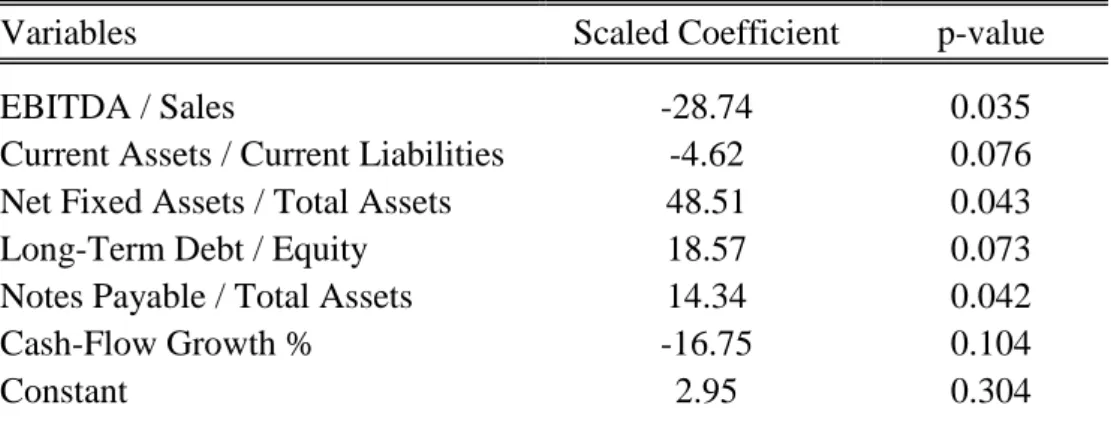
As result of their study, Platt and Platt (2002) presented, to what they referred as final model, The Early Warning System Model. As shown in Table 2.3.1, this model comprises six variables: one indicating profit margin, two measuring liquidity, two assessing leverage, and one describing growth. Financially distressed firms were coded as 1 and healthy firms were coded as 0, meaning that a positive coefficient indicated a straight liaison with financial distress while a negative coefficient indicated an inverse liaison to financial distress.

Table 2.3.1 - Variables in the Final Early Warning Model (2002)

Variables Scaled Coefficient p-value

EBITDA / Sales -28.74 0.035

Current Assets / Current Liabilities -4.62 0.076 Net Fixed Assets / Total Assets 48.51 0.043

Long-Term Debt / Equity 18.57 0.073

Notes Payable / Total Assets 14.34 0.042

Cash-Flow Growth % -16.75 0.104

Constant 2.95 0.304

Source: Adapted from Platt and Platt (2002)

EBITDA to Sales is referred as indicating profit margin, Current Assets to Current Liabilities (current ratio) and Net Fixed Assets to Total Assets are the variables measuring liquidity, Long-Term Debt to Equity and Notes Payable to Total Assets are the variables assessing leverage, and growth is described as Cash-Flow growth.

According to Platt and Platt (2002), it is more probable for a firm to be financially distressed if it had lower (or negative) operating cash flow (EBITDA) to sales, a lower current ratio, higher net fixed assets to total assets, higher long-term debt to equity, higher notes payable to total assets, and lower (or negative) cash flow growth from last period.

Platt and Platt (2002) concluded that the variables EBITDA to Sales, current ratio and the annual Cash Flow Growth Rate were negatively related to the probability that a firm would become financially distressed. This means that the higher these ratios were the less probable would be for a firm to experience financial distress. The other variables, Net Fixed Assets to

(36)

Total Assets, Long-Term Debt to Equity, and Notes Payable to Total Assets, were positively related to financial distress, meaning that the higher these ratios were the more probable was that a firm would experience financial distress.

Platt and Platt (2006) continued their examination on financial distress, and on their study addressed to the differences between financial distress and bankruptcy. The authors say that these two concepts are different. They found that bankruptcy and financial distress are not two sequential steps. Firms experience financial distress after poor operating results or due to external factors. On the other hand, bankruptcy is an action firms take to protect their assets from creditors.

As financial distressed firms not always become bankrupt, Platt and Platt (2006) investigated if some factors, acknowledged to be indicators of future bankruptcies, were also valid for the prediction of financial distress and vice-versa.

Platt and Platt (2006) defined as financial distressed firms those who met the following criteria:

 Negative EBITDA covering interest expense;  Negative EBIT;

 Negative net income before special items.

The authors used data from the years 1999 and 2000 for 14 manufacturing industries in a total of 1,403 firms, of which 276 were financially distressed. Firms were only considered as financially distressed if the above mentioned criteria was met in both years. If not, the firm would be considered as non-financially distressed.

The independent variables used by the authors, as explanatory variables, refer to 1998 financial statements, one year before the date when the firms are identified as financially distressed, allowing them to be used in an early warning models for financial distress. Platt and Platt (2006) have used as variables, measures for profitability, liquidity, operational efficiency, leverage and growth and tested them as potential factors of financial distress. Profitability, liquidity, operational efficiency, and growth are expected to be negatively related to financial distress, when leverage is expected to be positively related.

The logit model in Platt and Platt (2006) estimating the probability of financial distress, comprises the following variables, all of them statistically significant:

(37)

24  CF / Sales = Cash Flow to Sales (with CF = Net Income + Depreciation + Amortization),

measuring profit margin;

 EBITDA / TA = Earnings Before Interest, Tax, Depreciation and Amortization to Total Assets, measuring operating profitability;

 CLTD Due / TA = Current portion of long-term debt to Total Assets, measuring leverage;

 TIE = Times interest earned (Earnings Before Tax1_{/ Interest Expense), also measuring} leverage; and

 QR = Quick Ratio [(Current Assets – Inventories) / Current Liabilities], measuring liquidity.

The results show evidence that a higher (lower) cash flow to sales, a higher (lower) EBITDA to total sales and a higher (lower) times interest earned contribute to a lower (higher) probability of financial distress. On the other hand, a higher (lower) current portion of long-term debt to total assets contributes to a higher (lower) probability of financial distress. One particularity to be noted is the fact that a higher (lower) Quick Ratio (QR) contributes to a higher (lower) probability of financial distress. According to Platt and Platt (2006), this situation may be explained by the fact that if a firm invests in less profitable current assets in comparison to fixed assets it increases the chances of becoming financially distressed within one year.

The Final Early Warning Model had an overall correct classification rate of 93,2%.

In their study, Platt and Platt (2006) have also tested if there was a connection between financial distress and bankruptcy. In summary, the authors mentioned three possible views: 1. Financial distress and bankruptcy are part of a single on-going process, where it would be possible to assume the same factors to explain both;

1_{Earnings Before Tax = Net income +/- discontinued operations income/expense +/- extraordinary gains/losses}

+/- cumulative effect of accounting changes +/- tax benefits/expenses +/- minority interest + interest expense (Platt and Platt, 2006).

(38)

2. Financial distress and bankruptcy are similar processes, where there is a partial connection between the two processes, meaning that bankruptcy is a later stage of financial distress, but only the firms in financial distress that face other factors go bankrupt;

3. Financial distress and bankruptcy are different processes.

According to the results of their study, Platt and Platt (2006) conclude bankruptcy is not just a continuation process of financial distress. It is possible for firms to apply corrective measures that will help them overcome financial distress and become financially stronger. Hill, Perry and Andes (2011), on their research, used event history methodology and dynamic models to study both bankruptcy and financial distress. According to the authors, most of the distressed firms do not become bankrupt. Bankruptcy and financial distress are typically studied using multiple discriminant analysis and logit or probit models. With the use of event history methodology and dynamic models, the authors introduced time-varying explanatory variables and control for censored observations. Hill et al. (2011) consider bankruptcy to be an alteration in a firm’s financial situation, and for that reason it is relevant to test the explanatory financial variables prior to distress and bankruptcy have occurred. On their study, Hill et al. (2011) divided firms in the following categories: stable, financially distressed and bankrupt, pointing out that the variables that describe bankruptcy differ from the ones describing financial distress. The authors further mention that a bankruptcy prediction model that differentiates between financially distressed firms that persist and financially distressed firms that go bankrupt offers additional information to what is observed in the models that only compare stable and bankrupt firms. The authors have selected a sample of all NYSE and AMEX firms that went through financial distress at least once during 1977-1987. They describe as financially distressed firms those firms having cumulative negative earnings over any three-year period from 1977 to 1987.

On their model, Hill et al. (2011) used the following explanatory variables:  Liquidity variable: Cash to Total Assets;

 Profitability variable: Income before Extraordinary Items to Total Assets;  Leverage variable: Total Liabilities to Total Assets;

 Size variable: Natural Logarithm of Sales: and

(39)

26 Besides the firm’s financial information, the authors have also added two external variables: prime rate and unemployment rate. Their assumed that high interest rates and unstable unemployment rates affect the firm’s financial health.

For the entire sample, the authors conclude that five variables, liquidity, leverage, size, qualified opinion and prime rate, are statistically significant for financially distressed firms. For bankrupt firms, profitability, leverage, size, qualified opinion, the unemployment rate and prime rate are statistically significant.

(40)

3. Method variables and sample

3.1 Sample selection

3.1.1 Industry sel ection and financial distres s cri teri a

In a first phase, we have retrieved from the SABI financial database all Portuguese companies whose legal form was public limited company and limited liability company (corresponding to “Sociedade Anónima” and “Sociedade Limitada” in the Portuguese legal context, respectively) and with sales above EUR 2.5 million for the years 2006 to 2017. Afterwards, in order not to bias the study, all companies with the following activities were removed from the sample:

- Financial and insurance activities;

- Activities of head offices (e.g. holding companies); - Public administration and defence;

- Education activities;

- Arts, entertainment, sports and recreation activities; - Activities of membership organisations;

- Activities of households as employers;

- Activities of extraterritorial organisations and bodies.

This gave us an initial total sample of 245.290 firms’ year observations for this 12-year period.

Finally, we have decided to analyse companies only from the manufacturing industry1, belonging to 24 manufacturing industries listed in Table 3.3.3. The argument is based on the fact that we use financial data, where the lack of homogeneity in different sectors leads to considerable distortions in the results.

A winsorisation at 1% each tail was applied in order to reduce the effect of possibly spurious outliers.

(41)

28 Companies were classified as financially distressed and non-financially distressed as defined by Platt and Platt (2006), except for the third criteria1_:

• Negative EBITDA covering interest expense2; • Negative EBIT;

• Negative net earnings.

All the companies that met these three conditions consecutively for two consecutive years were identified as financially distressed.

3.1.2 Ti me p eri od s el ecti on

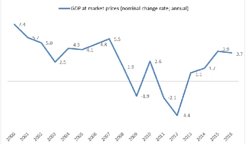
In our study, we have selected the years 2006-2008, 2010-2012 and 2014-2016. We have chosen these three periods to reflect in our work three distinct moments that have affected the Portuguese economy in recent years: pre/beginning of financial crisis (2006-2008), deepest period of the financial crisis (2010-2012) and post financial crisis (2014-2016). We have supported our time period selection with the annual nominal change rate of Gross domestic product (GDP) at market prices of the Portuguese economy, as seen in Figure 3.1.2.1:

Figure 3.1.2.1 GDP at market prices (nominal change rate; annual).

Source: Adapted from Instituto Nacional de Estatística (INE).

1_{In SABI database we are not able to collect the net income before special items.} 2_{EBITDA – interest expense (Platt and Platt, 2006).}

(42)

The years 2006, 2007, and 2008 reflect the period pre/beginning of the financial crisis. The years 2010, 2011 and 2012 reflect the full force of the impact of the financial crisis, with the GDP, at market prices, of the Portuguese economy suffering a significant decrease for the years 2011 and 2012. The years 2014, 2015 and 2016 already reflect the post financial crisis with a recovery of the GDP, at market prices, already started in 2013.

3.2 Variables definition and model applied

For the choice of the independent variables, we have used five variables that were present in the global financial distress prediction model of Platt and Platt (2008) and we have included seven additional independent variables.

The regressors included in our model, which were present on the global financial distress prediction (Platt and Platt, 2008) are:

 CF / S = Cash Flow to Sales (with CF = Net Income + Depreciation + Amortization);  EBITDA / TA = Earnings Before Interest, Tax, Depreciation and Amortization to Total

Assets;

 CA / CL = Current Assets to Current Liabilities;

 S / WC = Sales to Working Capital (With WC = CA – CL);

 DA / EBIT = Depreciation and Amortization to Earnings Before Interest and Tax. Additionally we have included new independent variables:

 STD / TA = Short-term Debt to Total Assets;  TE / TA = Total Equity to Total Assets;  EXPORTS = Sales from exportation to Sales;

 AGE, measuring the number of years the company is in activity;  GROWTH_TA, measuring the growth in Total Assets year-on-year;  GROWTH_S, measuring the growth in Sales year-on-year.

We have included these new variables due to the following reasoning:

 STD / TA comes as an alteration of the original variable included in Platt and Platt (2008) global financial distress prediction model: NP / TA (Notes Payable to Total Assets).

(43)

30 Since no information about Notes Payable was available on SABI database, we have decided to replace it for Short-term debt, allowing us to assess the statistical significance of short-term indebtedness in the prediction of financial distress. It is our expectation that STD / TA is positively correlated with financial distress as a higher level of leverage implies a higher channelling of operating cash flow to repay principal and associated interest expenses.  TE / TA, as it is our expectation that this variable is negatively correlated with financial distress, as a higher Equity Ratio implies a lower dependence of external funding and therefore a lower allocation of operating cash flow to the reimbursement of debt with external parties. It is also an indication that previous net profits are being retained in the firm and not being channelled to the shareholders by the way of dividends.

 EXPORTS, as we expect the level of the internationalization of the activity (exportation) to be negatively correlated with financial distress. The higher the level of exportations of a given firm, the lower the dependence of the domestic market. In case the domestic market is in contraction, a firm in which a significant part of its sales is generated from external markets will be in a better position to maintain a stable sales and operating cash flow levels.  AGE, as we expect a firm that is operating for a longer period of time to have more experience and knowledge of the market(s) where it operates. We therefore expect this variable to be negatively correlated with financial distress.

 GROWTH_TA and GROWTH_S: growth in Total Assets as a measure of the firm’s capacity to invest on its asset base and growth in Sales as a measure of the firm’s capacity to expand its activity. We expect these two variables to be negatively correlated with financial distress as they both reveal that the firm has been able to grow.

As we consider the legal form of a firm to be relevant for the prediction of financial distress in the Portuguese economic context, we have also included as independent variable a dummy variable “SA” which corresponds to firms whose legal form is “Sociedade Anónima”. If the company’s legal form is “Sociedade Anónima”, SA=1, and if not, SA=0.

We expect this variable to be positively correlated with financial distress, as in firms whose legal form is “Sociedade Anónima” the management board is often professionalised and dissociated with the shareholders. This means that there might be conflicts of interest between the shareholders and the management board, which may lead to financial distress. On the other hand, in companies whose legal form is “Sociedade Limitada”, the management

(44)

board is often composed by the shareholders, with minimized or inexistent conflict of interests.

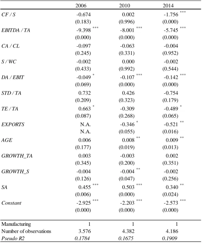
Regarding the model employed, with the statistical software STATA, we have applied a logit regression using the above mentioned independent variables based on the financial data one year before the date when the firms are identified as financially distressed.

3.3 Results

The explanatory variables come from 2006, 2010 and 2014 financial statements, one year before the date when the firms are identified as financially distressed.

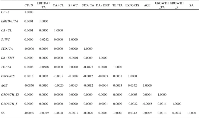
As shown in Table 3.3.1, Table 3.3.2, and Table 3.3.4, we have tested 12 variables: one indicating profit margin (CF/S), one measuring liquidity (CA/CL), one measuring operating profitability (EBITDA/TA), one measuring internationalisation (EXPORTS), two assessing leverage (STD/TA and TE/TA), one measuring operating efficiency (S/WC), one measuring operating leverage (DA/EBIT), two describing growth (GROWTH_TA and GROWTH_S), one describing age (AGE) and one describing the legal form (SA). Financially distressed firms were coded as 1 and healthy firms were coded as 0, meaning that a positive coefficient indicated a straight liaison with financial distress while a negative coefficient indicated an inverse liaison to financial distress.

Table 3.3.1 – Variables Correlation

CF / S EBITDA /

TA CA / CL S / WC STD / TA DA / EBIT TE / TA EXPORTS AGE

GROWTH _TA GROWTH _S SA CF / S 1.0000 EBITDA / TA 0.0001 1.0000 CA / CL 0.0001 0.0000 1.0000 S / WC 0.0000 -0.0242 0.0000 1.0000 STD / TA -0.0006 0.0099 0.0000 0.0000 1.0000 DA / EBIT 0.0000 0.0000 0.0000 -0.0001 0.0000 1.0000 TE / TA 0.0008 -0.0608 0.0000 0.0000 -0.4873 0.0001 1.0000 EXPORTS 0.0013 0.0007 -0.0017 -0.0009 -0.0012 -0.0003 0.0031 1.0000 AGE -0.0850 0.0010 -0.0020 0.0013 -0.0012 -0.0004 0.0033 0.0352 1.0000 GROWTH_TA 0.0000 0.0000 0.0000 0.0000 0.0000 0.0000 0.0000 -0.0003 0.0004 1.0000 GROWTH_S 0.0000 0.0000 0.0000 0.0000 0.0000 -0.0001 0.0000 -0.0022 -0.0055 0.0014 1.0000 SA -0.0035 -0.0019 -0.0031 -0.0012 -0.0020 0.0006 -0.0001 0.0342 0.0909 0.0013 0.0037 1.0000

(45)

32 In Table 3.3.1 it can be seen that only two variables present a strong correlation (TE/TA and STD/TA), which is not unexpected given that both aim to capture a measure of a firm’s leverage (one through the equity ratio and other through the level of short term indebtedness). This does not affect the explanatory power of the model, as the correlation between all the other variables is weak, with each variable explaining a different reality.

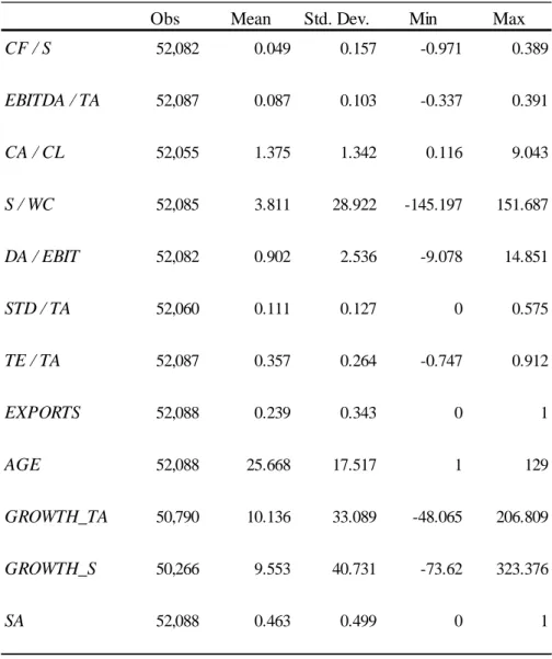
Table 3.3.2 – Sample Characteristics

Obs Mean Std. Dev. Min Max

CF / S 52,082 0.049 0.157 -0.971 0.389 EBITDA / TA 52,087 0.087 0.103 -0.337 0.391 CA / CL 52,055 1.375 1.342 0.116 9.043 S / WC 52,085 3.811 28.922 -145.197 151.687 DA / EBIT 52,082 0.902 2.536 -9.078 14.851 STD / TA 52,060 0.111 0.127 0 0.575 TE / TA 52,087 0.357 0.264 -0.747 0.912 EXPORTS 52,088 0.239 0.343 0 1 AGE 52,088 25.668 17.517 1 129 GROWTH_TA 50,790 10.136 33.089 -48.065 206.809 GROWTH_S 50,266 9.553 40.731 -73.62 323.376 SA 52,088 0.463 0.499 0 1