SoilS: prediction of cadmium adSorption
giuliano marchi(1)*, cesar crispim Vilar(2), george o’connor(3), letuzia maria de oliveira(3), adriana reatto(1) and thomaz adolph rein(1)
(1) Empresa Brasileira de Pesquisa Agropecuária, Embrapa Cerrados, Brasília, Distrito Federal, Brasil. (2) Universidade do Estado de Mato Grosso, Campus Nova Xavantina, Nova Xavantina, Mato Grosso, Brasil. (3) University of Florida, Soil and Water Sciences Department, Gainesville, Florida, United States.
* Corresponding author.
E-mail: [email protected]
abStract
intrinsic equilibrium constants for 22 representative brazilian oxisols were estimated from a cadmium adsorption experiment. Equilibrium constants were fitted to two surface complexation models: diffuse layer and constant capacitance. intrinsic equilibrium constants were optimized by fiteQl and by hand calculation using Visual minteQ in sweep mode, and excel spreadsheets. data from both models were incorporated into Visual minteQ. constants estimated by fiteQl and incorporated in Visual minteQ software failed to predict observed data accurately. however, fiteQl raw output data rendered good results when predicted values were directly compared with observed values, instead of incorporating the estimated constants into Visual minteQ. intrinsic equilibrium constants optimized by hand calculation and incorporated in Visual minteQ reliably predicted cd adsorption reactions on soil surfaces under changing environmental conditions.
Keywords: intrinsic equilibrium constants, oxisol, fiteQl, Visual minteQ, chemical equilibrium software.
reSumo: ModelageM por CoMplexação de SuperfíCie eM SoloS de Carga VariáVel: predição da adSorção de CádMio
Constantes de equilíbrio intrínsecas de 22 latossolos brasileiros representativos da região do Cerrado foram estimadas por meio de um experimento de adsorção de cádmio. as constantes de equilíbrio foram ajustadas a dois modelos de superfície de complexação: camada difusa e capacitância constante. as constantes
introduction
Anthropogenic activities, such as mining or industrial activities, agricultural chemical applications - mainly phosphate and zinc micronutrients (Guilherme et al., 2014), and organic and inorganic residue application to soils may cause cadmium (Cd) concentration to build up over time. Cadmium is bound to the solid phase of soils as a result of surface precipitation and adsorption processes. Its mobility and destination in the soil environment are directly related to processes that are highly pH dependent (Lee et al., 1996).
Soil contamination by Cd is of great concern in terms of its entry into the food chain for it can be taken up by food plants in large amounts relative to its concentration in the soil. Furthermore, Cd accumulates over a lifetime in the body (ATSDR, 2012) and has adverse health effects, mainly in the form of renal dysfunction (Hooda, 2010). Environmental and human health risk assessment of metals depends to a great extent on modeling the destination and mobility of metals based on soil-liquid partitioning coefficients (Sauvé et al., 2000) that can be estimated locally.
Cadmium adsorption is mainly controlled by soil organic matter (Lee et al., 1996; Shi et al., 2007), pH (Sauvé et al., 2000), cation exchange capacity, clay content or type, surface area (Appel and Ma, 2002), surface charge (He et al., 2005), or a combination of those soil components. Different components in soils may contribute to Cd adsorption to different extents (Shi et al., 2007). Indeed, controlling the factors of Cd adsorption in highly weathered soils, such as Oxisols, are not clear (Alleoni and Camargo, 1994). Correlation coefficients between Cd adsorption and many soil properties for 17 Oxisols were inconclusive at pH 4.5, but highly significant at pH values of 5.5 and 6.5. Properties such as surface area, CEC, clay, kaolinite, and hematite contents were highly correlated (Pierangeli et al., 2003), emphasizing the importance of pH, surface area, and charge for Cd adsorption in these soils. Understanding mechanisms of metal adsorption in soils is important
as these reactions control the strength of the metal-soil surface interactions (He et al., 2005).
Oxisols are characterized by B horizons with 1:1 clay minerals and variable amounts of Fe and Al hydrous oxides (Reatto et al., 2009a), exhibiting generally low surface charge density with predominant pH-dependent surface charge. Charge develops from protonation and deprotonation reactions of hydroxyl groups protruding from the surfaces of the minerals, and by deprotonation of acidic functional groups exposed on the surfaces of solid organic matter (Charlet and Sposito, 1987).
Little research has been done directly comparing surface charge with heavy metal sorption in variable charge systems (Appel and Ma, 2002). In this regard, surface complexation models have distinct advantages over empirical models (which provide soil-liquid partitioning coefficients for further modeling) because surface complexation models can be extrapolated to systems of different ionic strengths, pH’s, and component compositions (Koretsky, 2000; Bethke, 2008). However, application of the surface complexation modeling approach to natural systems, such as soils, is considerably more difficult, and rare, than application to simple mineral-water systems (Davis and Kent, 1990; Davis, 2001). Theory needs to describe hydrolysis and the mineral surfaces, account for electrical charge, and provide for mass balance on the sorbing sites. In addition, an internally consistent and sufficiently broad database of sorption reactions should accompany the theory (Bethke, 2008). Estimated intrinsic equilibrium constants must ultimately describe reliable results within chemical speciation software packages, such as Visual MINTEQ (Gustafsson, 2014), allowing end users to perform predictions and apply results in further technologies.
Intrinsic equilibrium constants estimated from Cd adsorption in soils, optimized by FITEQL and by hand calculation may be incorporated into Visual MINTEQ. Results may be validated as comparing observed results of Cd adsorption in four Oxisols with those predicted by Visual MINTEQ.
The overall objectives of this study were to estimate intrinsic equilibrium constants of Cd de equilíbrio intrínsecas foram otimizadas pelo programa fiTeQl e pelo cálculo manual usando o programa Visual MiNTeQ no modo “sweep” e planilhas do excel. dados dos dois modelos foram incorporados ao Visual MiNTeQ. as constantes estimadas pelo fiTeQl e incorporadas ao Visual MiNTeQ falharam ao predizer acuradamente os dados observados. entretanto, os dados brutos de saída do fiTeQl geraram bons resultados quando os valores preditos foram comparados diretamente aos observados, em vez de incorporar as constantes estimadas ao Visual MiNTeQ. a predição das reações de adsorção de Cd na superfície do solo pelas constantes de equilíbrio intrínsecas otimizadas pelos cálculos manuais e incorporadas ao Visual MINTEQ foram confiáveis e podem ser utilizadas sob diversas situações ambientais.
adsorption for 22 Oxisols, incorporate them into chemical speciation software, such as Visual MINTEQ, and validate the results, comparing observed results of Cd adsorption in four Oxisols with those predicted by Visual MINTEQ software.
material and methodS
Soil samples and properties
Soil samples from the 0.00-0.20 m depth from 20 sites were collected and characterized for mineralogy, texture, organic carbon, and cation exchange capacity at pH 7.0 by Rein (2008); additional soils from horizons A and Bw from three sites were collected and characterized by Reatto et al. (2007, 2008, 2009a,b). The characterization data, displayed in tables 1 and 2, were used in the present study. Site location was based on survey reports to provide a representative sample of pristine Cerrado (tropical savanna) Oxisols from Brazil. Consideration was given to geographic distribution, variations in texture, mineralogical composition of the clay fraction, and parent material. All sampled sites were under native vegetation, and had never been cropped or amended.
Determination of surface area was performed as described by Cerato and Lutenegger (2002), with modifications. Soil was passed through a 2 mm sieve, oven dried for 12 h at 120 ºC to remove water, and then placed (1 g) in an aluminum tare. Three mL of ethylene glycol monoethyl ether (EGME) were mixed with the soil. Tares were placed in a desiccator and a 635 mm Hg vacuum was applied. One hundred and 10 grams of oven-dried CaCl2 was used as a desiccant. After 18 and 24 h, the desiccator was opened and the tares were weighed. If the mass of the sample varied more than 0.001 g from the first time to the second, the sample was placed once more in the desiccator and evacuated again for 4 h more. The procedure was repeated successively until the tares reached constant weight. Soil surface area (a)
was calculated as A
Wa
=
Ws
2.86 × 10⁻⁴ , where Wa is
the weight of EGME retained by the sample in g; Ws is the oven dry weight of soil; and 0.000286 is t h e w e i g h t o f E G M E r e q u i r e d t o f o r m a monomolecular layer on a square meter of surface (m2 g-1). Reference clays from the Source Clay Mineral Repository at the University of Missouri at Columbia, Missouri, USA, were used to validate the method.
adsoption isotherms
Cadmium adsorption envelopes (amount of Cd adsorbed as a function of solution pH at a fixed total Cd concentration) were determined
for all soil samples. One g of soil was placed in polypropylene centrifuge tubes and brought to equilibrium with 15 mL of a 0.1 mol L-1 NaCl. Tubes were agitated at 200 rpm for 12 h in a reciprocating shaker. Acid or base were added, and the operation was repeated several times, up to 72 h total time, to adjust initial suspension pH values to 4.5, 5.0, 5.5, 6.0, and 6.5. Each treatment had three replications. Five mL of 0.36 mmol L-1 Cd solution in 0.1 mol L-1 NaCl was mixed with the soil suspensions. Final Cd concentration in the soil suspension was 0.09 mmol L-1. Soil suspensions were shaken at 200 rpm for 24 h, and the pH of suspensions at the end of this procedure was recorded. Soil suspensions were centrifuged at 8000 rpm for 10 min, and the supernatant was collected for Cd analysis by inductive coupled plasma with mass spectrometry (ICP-MS).
A review of the theory and assumptions of the constant capacitance model, as well as of the diffuse layer model was presented in Goldberg (1992). The soil will be considered as an integrated whole with an average surface functional group (expressed as SOH). The surface protonation and deprotonation of the soil are expressed as equations 1 and 2:
SOH2+=SOH+H+ Eq. 1
SOH=SO−+H+ Eq. 2
The adsorption of Cd on the soil surface is expressed by the following surface complexation reaction (Equation 3).
SOH+Cd2+=SOCd++H+
Eq. 3
Other reactions with Cd and Cl- were also included in the modeling, e.g., CdCl+ and CdCl
2 species played an important role in solution equilibria (equations summarized in table 3), even though CdCl+ was not considered as a surface-bound species.
Intrinsic equilibrium constant expressions for the surface complexation reactions are:
Ka
SOH
SOH H
F
RT int
+
+
+
=
2
exp Ψ Eq. 4
Ka
SO H
SOH RT
int
−
− +
=
−
[ ]
exp
FΨ Eq. 5
K
SOCd H
SOH Cd
SOCd
int =
+ +
+
2 Eq. 6
Optimal best-fit values for the surface site acidity constants, log Ka1
int
and log Ka2
int
, as well as surface site density for Oxisols from the Brazilian Cerrado, were calculated from a previous study (Table 1). These constants were fixed when the metal binding constants were calculated from the batch adsorption data.
The Davies equation (Davies, 1938)and a revision of the dissociation constants of some sulphates Journal of the Chemical Society (Resumed and the specific interaction theory (Sukhno and Buzko, 2004), both used for activity correction in Visual MINTEQ, were applied to adjust activity coefficients in extrapolation of equilibrium constants in i = 0.1 mol L-1 (Table 3). Equilibrium constants of dissolved species extrapolated to i = 0.1 mol L-1 by the Davies equation (Equation 7) were used to optimize log KSoCd
int
by FITEQL 4.0 (Herbelin and Westall, 1999), and were used in further modeling through Visual MINTEQ. There is no generally accepted convention
for treating activity coefficients of surface species (Richter et al., 2005). In general, there is little or no change in the pH dependence of adsorption with ionic strength (between 0.001-1.0 mol L-1) for specifically adsorbed ions like Cu2+, Pb2+, Ni2+, and Cd2+ (Hayes and Leckie, 1987); therefore, adopted protonation/dissociation constants were obtained from a previous study in 0.1 mol L-1 NaCl. The Davies equation is:
√ + √
lo γ z I .
I I
0 5
1 0 3
2
Eq. 7
where the subscript i refers to each of the reactants and products in the reaction; zi is the ionic charge of each reactant or product; and i is the ionic strength reported for the experimental data.
Once computed, the activity coefficients were used in the following relationship to correct the equilibrium constants to I = 0.1 mol L-1:
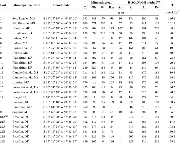
table 1. Selected soil mineralogical and chemical properties
Soil municipality, State coordinate mineralogical
(3) h
2So4/naoh method(4)
t ct gb gt hm an Si al fe
g kg-1 mmolc kg-1
1(1) Sete Lagoas, MG S 19° 27’ 18’’ W 44° 11’ 01’’ 691 141 75 69 16 134 200 88 136.4
2 São Gotardo, MG S 19° 16’ 50’’ W 46° 09’ 13’’ 108 571 206 34 57 23 241 133 101.9
3 Uberaba, MG S 19° 42’ 13’’ W 47° 57’ 35’’ 228 262 193 179 107 45 151 205 38.9
4 Itumbiara, GO S 18° 17’ 07’’ W 49° 14’ 21’’ 173 399 242 109 56 35 198 197 90.8
5 Balsas, MA S 07° 27’ 41’’ W 46° 01’ 04’’ 921 0 91 0 17 164 184 48 20.9
6 Balsas, MA S 08° 30’ 55’’ W 46° 44’ 55’’ 665 196 95 42 17 128 211 77 66.9
7 Correntina, BA S 13° 47’ 36’’ W 45° 52’ 56’’ 865 15 83 13 25 151 180 51 19.3
8 Buritis, MG S 15° 21’ 24’’ W 46° 41’ 38’’ 603 324 57 0 28 110 240 31 40.6
9 Planaltina, DF S 15° 36’ 53’’ W 47° 45’ 02’’ 355 507 112 0 23 69 261 60 75.5
10 Planaltina, DF S 15° 35’ 55’’ W 47° 42’ 28’’ 634 195 61 108 17 112 208 106 79.2
11 Planaltina, DF S 15° 36’ 36’’ W 47° 44’ 14’’ 259 529 185 0 19 44 240 93 44.7
12 Campo Grande, MS S 20° 25’ 03’’ W 54° 42’ 01’’ 511 139 165 152 33 95 170 185 89.3
13 Campo Grande, MS S 20° 25’ 40’’ W 54° 43’ 28’’ 623 102 88 156 25 117 176 152 99.6
14 Itiquira, MT S 17° 26’ 41’’ W 54° 15’ 51’’ 776 41 58 103 19 138 175 99 45.7
15 Porto Nacional, TO S 10° 31’ 35’’ W 48° 20’ 30’’ 425 403 149 0 23 76 236 78 46.5
16 Porto Nacional, TO S 10° 56’ 19’’ W 48° 18’ 07’’ 630 251 60 55 17 113 215 69 26.5
17 Uruçuí, PI S 07° 28’ 07’’ W 44° 16’ 32’’ 839 1 150 0 23 154 177 75 64.8
18 Panamá, GO S 18° 11’ 46’’ W 49° 17’ 00’’ 430 222 107 189 30 82 180 181 153.7
19 Canarana, MT S 13° 31’ 29’’ W 52° 19’ 02’’ 250 522 68 121 21 46 240 119 71.8
20 Sapezal, MT S 13° 32’ 23’’ W 58° 29’ 58’’ 504 309 84 78 19 93 222 99 95.6
21A(2) Brasília, DF S 15° 36’ 92’’ W 47° 45’ 78’’ 355 514 131 0 - 212 610 151 59.5
21B Brasília, DF S 15° 36’ 92’’ W 47° 45’ 78’’ 412 442 146 0 - 239 564 163 17.5
22A Brasília, DF S 15° 13’ 24’’ W 47° 42’ 15’’ 561 273 112 54 - 315 482 187 108.1
22B Brasília, DF S 15° 13’ 24’’ W 47° 42’ 15’’ 591 241 93 75 - 327 465 188 30.6
23A Brasília, DF S 15° 14’ 08’’ W 47° 46’ 37’’ 474 326 55 145 - 265 481 233 169.3
23B Brasília, DF S 15° 14’ 08’’ W 47° 46’ 37’’ 399 405 0 196 - 226 514 239 55.9
(1) Soils no. 1-20, data from Rein (2008); (2) Soils no. 21-23, data from Reatto et al. (2008); letters A and B, mean horizons A and B of
soils; (3) HF-microwave, chemical allocation method (Resende et al., 1987); Kt: kaolinite; Gb: gibbsite; Gt: goethite; Hm: hematite;
An: anatase; (4) H
K
IK
I i i products vi i reactants v
=
=
0 '
γ
γ
,,
Eq. 8
where v represents the reactant or product stoichiometric coefficient.
The dominant Cd solution species in groundwater at pH values greater than 8.2 is CdCO3 (aq). Precipitation with carbonate is increasingly important in systems with a pH greater than 8 (USEPA, 1999). However, Brazilian Oxisols are rather acidic soils; therefore, the effect of partial CO2 pressure, and its related compounds, in simulated suspensions was not included in Visual MINTEQ or FITEQL calculations.
The FITEQL program was used to optimize surface complexation modeling of the experimental Cd adsorption. The program was set to allow ionic strength and activity corrections. FITEQL uses the Davies equation to correct ionic activity (Equation 7). Obtained equilibrium constants were
averaged using the weighting method of Dzombak and Morel (1990), in which the weighting factor wi is defined as:
w
i
K i
log K i
=
(
)
∑
(
)
1
1 /
/
log
σ
σ Eq. 9
where (σlog K)i is the standard deviation of log K calculated by FITEQL for the ith data set. The best estimate for log K is then calculated as:
logK wi logK
i
= ∑
(
)
Eq. 10Another method to optimize log KSoCd
int
values was employed. Using observed data as a guide parameter, simulations with Visual MINTEQ were used to optimize by trial and error (systematic variations of assumed values of log KSoCd
int
) using the method of least squares regression (with a log KSoCd
int precision of 0.01). This method seeks to minimize the sum of the squared errors (SSE) between observed and calculated values of the dependent variable, in this case the sorbed Cd concentration, S (Bolster and Hornberger, 2007):
SSE Si Si
i N
= −
=
∑
1 2
[ ] Eq. 11
where SSE is the objective function to be minimized; N is the number of observations; Si is the ith measured value of the dependent variable; and Si is the ith model-predicted value of the dependent variable.
The constant capacitance model is very insensitive to values of capacity density (C1) (Goldberg, 1995). The choice of the C1 value is arbitrary, and it is recommend to use the best fit values (~1.0 F m-2) (Hayes et al., 1991). We chose to use the C1 value of 1.06 F m-2 (derived from Al oxides) (Westall and Hohl, 1980), which is usually used for soil modeling (Goldberg et al., 2000).
Intrinsic equilibrium constants passed through Dixon’s outlier and normality (Shapiro-Wilk and Lilliefors) tests using PROUCL software (Maichle and Singh, 2013).
Validation
The validation of the surface complexation models obtained with adsorption of Cd in 16 soil samples collected by Rein (2008) and six by Reatto et al. (2008) was carried out using four soil samples from different localities (Sete Lagoas, São Gotardo, Uberaba, and Itumbiara), collected in a transect by Rein (2008). These four soil samples were not used during model prediction. The set up for the validation experiments was the same as that used for prediction. All model parameters have been maintained unvaried; therefore, the results presented are a test of the ability of the model to simulate Cd adsorption in these four soils.
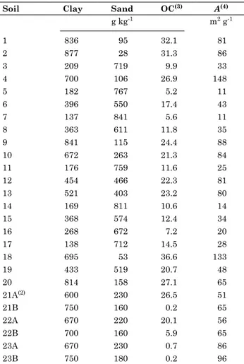
table 2. Soil texture, organic matter content and surface area
Soil clay Sand oc(3) A(4)
g kg-1 m2 g-1
1 836 95 32.1 81
2 877 28 31.3 86
3 209 719 9.9 33
4 700 106 26.9 148
5 182 767 5.2 11
6 396 550 17.4 43
7 137 841 5.6 11
8 363 611 11.8 35
9 841 115 24.4 88
10 672 263 21.3 84
11 176 759 11.6 25
12 454 466 22.3 81
13 521 403 23.2 80
14 169 811 10.6 14
15 368 574 12.4 34
16 268 672 7.2 20
17 138 712 14.5 28
18 695 53 36.6 133
19 433 519 20.7 48
20 814 158 27.1 65
21A(2) 600 230 26.5 51
21B 750 160 0.2 65
22A 670 220 20.1 56
22B 700 160 5.9 65
23A 670 230 0.7 86
23B 750 180 0.2 96
(1) Soils no. 1-20, data from Rein (2008); (2) Soils no. 21-23, data
from Reatto et al. (2008); letters A and B, mean horizons A and B of soils; (3) Organic carbon (Embrapa, 1979); (4)a: specific surface
Observed vs. predicted plots of Cd adsorption values from this series of soils were compared using the root mean square error (RMSE) and a dimensionless statistic which directly relates model predictions to observed data such as modeling efficiency (EF) (Mayer and Butler, 1993):
RMSE ŷ y
n
i N
i i
=
(
−)
=
∑
12 0 5.
Eq. 12
where yi represents observed values; ŷi, simulated values; and n, the number of pairs.
E F ŷ y ŷ y
i N
i i
i N
i
= −
(
−)
−(
)
=
=
∑
∑
1 1
2
1
2
Eq. 13
where ¯y represents the observed mean.
reSultS and diScuSSion
isotherms and constants
Measured surface areas (average ± standard deviation, n = 20) from kaolinite (KGa-2) and a Ca-Montmorilonite (SAz-1) were 44.75 ± 8.16 and 806.03 ± 53.11 m2 g-1, respectively. The values are close to the theoretical values for the clay minerals, and to reported values (van Olphen and Fripiat, 1979; Cerato and Lutenegger, 2002; Kennedy and Wagner, 2011).
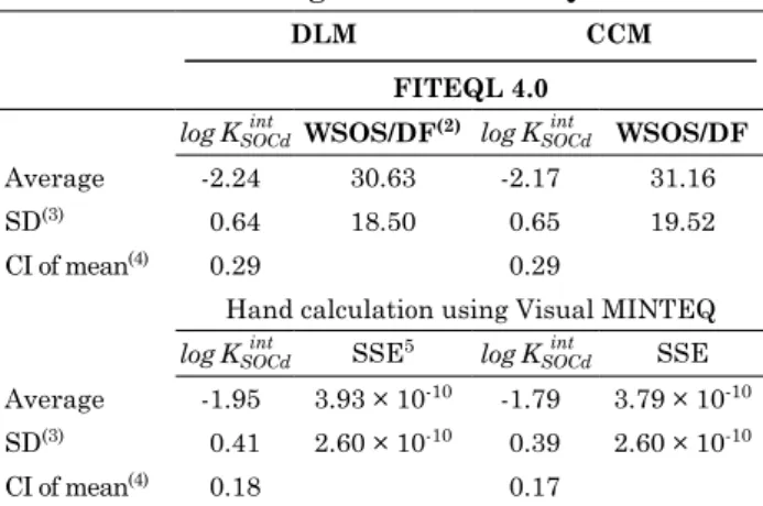
Intrinsic equilibrium constants estimated by FITEQL were 0.29 and 0.38 units smaller for DLM and CCM, respectively, than those calculated by hand (Table 4). Confidence intervals were also narrower for the hand calculation group than those calculated by FITEQL. Very similar statistical results (standard deviation and confidence intervals) were found for DLM and CCM. Intrinsic equilibrium constants optimized by FITEQL and hand calculation differed significantly (Table 4).
A possible explanation for the difference between log KSoCd
int
results from FITEQL and from hand calculation using Visual MINTEQ may be related to FITEQL numerical instability or convergence problems (Villegas-Jiménez and Mucci, 2009). Speciation constants for major reactions used in FITEQL exactly matched those in Visual MINTEQ (Table 3). Output data from FITEQL, however, was able to predict the observed data with precision (Figure 1), and preliminary tests optimizing constants without taking into account background ionic strength (0.1 mol L-1 NaCl; in both software programs, FITEQL and Visual MINTEQ) were satisfactory, and predicted the observed results perfectly, but they did not correspond to reality. When optimized intrinsic equilibrium constants estimated by FITEQL were added to the Visual MINTEQ database including background ionic strength data, the program failed to accurately predict observed results of Cd adsorption (Figures 2 and 3). Some authors use site density to ultimately optimize curve fitting (Davis and table 3. proton and metal binding parameters used in the model for metal adsorption(1) onto oxisols
from the brazilian cerrado
Surface acidity constant(2) input parameter
Diffuse layer model
log Ka1
int = 2.93
log Ka2
int = -5.92
Site concentration (mmol kg-1) = 109.9
Constant capacitance model
log Ka1
int = 3.51
log Ka2
int = -5.94
Site concentration (mmol kg-1) = 113.7
Capacitance (F m-2) = 1.06
Common input parameter(3)
Reaction log K
I(4) = 0 i = 0.1 (Davies)(5) i = 0.1 (SIT)(6) Cd2+ + Cl- = CdCl+
(aq) 1.980 2.410 2.397
Cd2+ + 2Cl- = CdCl
2(aq) 2.600 3.244 3.206
Cd2+ + oH- = CdoH+
(aq) -10.097 -9.667 -9.691
Cd2+ + oH- = CdoH
(aq)
3+ -9.397 -9.397 -9.440
Cd2+ + 2oH- = Cd(oH)
2(aq) -20.294 -19.650 -19.690
Cd2+ + 3oH- = Cd
2(oH)
+
3(aq) -33.3 -32.656 -32.702
Na+ + oH- = NaoH
(aq) -13.897 -13.682 -13.687
Na+ + Cl- = NaCl
(aq) -0.300 -0.085 -0.089
H20 + H20 = H30 + OH- -13.997 -13.782 -13.796
(1) Suspension concentration = 50 g L-1; site concentration (Nt; mol kg-1) may be converted to site density (Ns; sites nm-2) by the following
Kent, 1990) because as site density increases, the adsorption edge shifts to lower pH values, whereas with decreasing site density, the adsorption edge shifts to higher pH values, allowing the modelist to adjust curve fitting “manually”. Using changes in site density to adjust curve fitting was not our intent in the present study. Rather, we searched for a hand calculation method that could provide more accurate results when using Visual MINTEQ, and that could be used as a reference, since as it was optimized accessing by Visual MINTEQ data directly (Table 4).
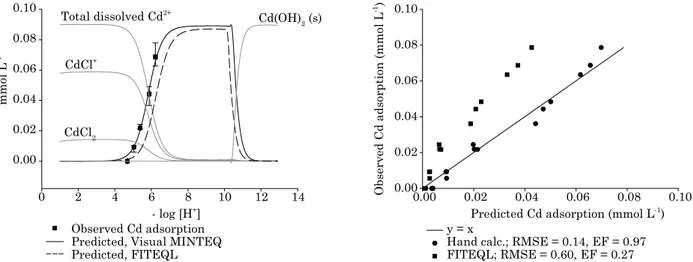
Intrinsic equilibrium constants optimized by hand calculation, considering a 0.1 mol L-1 NaCl background, was incorporated in the Visual MINTEQ database. The results showed good precision in reproducing the observed values (Figures 2 and 3). Using this approach, the diffuse layer and constant capacitance models produced very similar results. In fact, differences between models are insignificant (Davis and Kent, 1990) when models have matching pH and ionic strength. A sample from an Oxisol from Buritis, MG, based on estimated parameters from hand calculation, exhibited values of 0.14 and 0.15 for RSME for Cd adsorption, and 0.97 and 0.96 for EF in regard to DLM and CCM, respectively, showing very similar prediction values between models (Figures 2 and 3). When parameters estimated from FITEQL were added to Visual MINTEQ, RSME was high, and EF was low for both DLM and CCM (Figures 2 and 3). The latter statistical results clearly show disagreement among FITEQL optimization of log KSoCd
int
added into Visual MINTEQ and observed data (Figures 2 and 3).
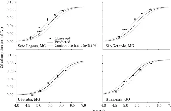
Validation
Cadmium adsorption in four Oxisol samples collected in Sete Lagoas, MG; São Gotardo, MG;
Uberaba, MG; and Itumbiara, GO, was modeled using parameters estimated by hand calculation in Visual MINTEQ (Table 4, Figure 4). Parameters derived from adsorption obtained at several fixed pH values were incorporated in the DLM to reproduce pH edge curves. Only DLM using optimization by hand calculation was shown in figure 4 since DLM and CCM showed equivalent results (Figure 1). Another reason for showing only DLM using optimization by hand calculation in figure 4 was that FITEQL optimized log KSoCd
int
values incorporated in Visual MINTEQ
table 4. average intrinsic equilibrium constants for cd adsorption onto 20 oxisols from the brazilian cerrado using the diffuse layer model (dlm) and the constant capacitance model (ccm), estimated by fiteQl 4.0 and by hand calculation using Visual minteQ(1)
dlm ccm
fiteQl 4.0 log KSoCdint WSoS/df(2) log K
SoCdint WSoS/df Average -2.24 30.63 -2.17 31.16
SD(3) 0.64 18.50 0.65 19.52
CI of mean(4) 0.29 0.29
Hand calculation using Visual MINTEQ
log KSoCdint SSE5 log KSoCdint SSE Average -1.95 3.93 × 10⁻¹⁰ -1.79 3.79 × 10⁻¹⁰
SD(3) 0.41 2.60 × 10⁻¹⁰ 0.39 2.60 × 10⁻¹⁰
CI of mean(4) 0.18 0.17
(1) Suspension concentration = 50 g L-1; Capacitance of inner
Helmholtz layer = 1.06 F m-2; Site density = 0.4295 and 0.4444 sites
nm-2 for DLM and CCM, respectively; (2) WSOS is the weighted
sum of squares of the residuals and DF is the degrees of freedom;
(3) SD: standard deviation from log K values; (4) CI of mean = 95 %
confidence interval; (5) SSE: sum of the squared errors.
figure 1. cadmium adsorption as a function of ph in an oxisol from buritis, mg, brazil, using observed and fiteQl output data: dlm = diffuse layer model and ccm = constant capacitance model (capacitance of inner helmholtz layer = 1.06 f m-2); Suspension concentration = 50 g l-1; surface
area = 35.22 m2 g-1; 0.1 mol l-1 NaCl; RMSE = root mean square error; EF = model efficiency.
Predicted Cd adsorption (mmol L-1)
0.00 0.02 0.04 0.06 0.08 0.10
Observed Cd adsorption (mmol L
-1 )
0.00 0.02 0.04 0.06 0.08 0.10
-log [H+]
4.5 5.0 5.5 6.0
Cd adsorption (mmol L
-1)
0 1e-1
(a) (b)
8e-2
6e-2
4e-2
2e-2
SOCd+ (predicted, DLM)
Observed Cd adsorption
SOCd+ (predicted CCM)
CCM; RMSE = 0.17, EF = 0.97 DLM; RMSE = 0.15, EF = 0.97
resulted in high RMSE and low EF values (Figures 2 and 3), contrasting with low RMSE and high EF obtained using hand calculation optimized log KSoCd
int values incorporated in Visual MINTEQ. Confidence limits were calculated from log KSoCd
int
dispersion (obtained from optimization of Cd adsorption in those 22 soil samples by hand calculation for the DLM) plotted against pH (Figure 4). Although it is interesting to know the likely range of a true value using log KSoCd
int
, it is important to show that each value of log KSoCd
int
is related to its soil surface
area. Therefore, the confidence interval established using only one value of soil surface area (from the sample under analysis) shows narrowed confidence intervals. Taking soil surface area into account, calculated confidence limits would probably show larger intervals. Therefore, another model of goodness of fit statistics was assessed, for purposes of validation, using RMSE and EF (Equations 12 and 13). In the end, cadmium adsorption was modeled satisfactorily in all four soils, according to validation statistics (Figure 5).
- log [H+]
0 2 4 6 8 10 12 14
mmol L
-1
0.00 0.02 0.04 0.06 0.08 0.10
Total dissolved Cd2+
CdCl+
CdCl2
Cd(OH)2 (s)
Predicted, FITEQL Observed Cd adsorption Predicted, Visual MINTEQ
Predicted Cd adsorption (mmol L-1)
0.00 0.02 0.04 0.06 0.08 0.10
Observed Cd adsorption (mmol L
-1)
0.00 0.02 0.04 0.06 0.08 0.10
y = x
Hand calc.; RMSE = 0.14, EF = 0.97 FITEQL; RMSE = 0.60, EF = 0.27
figure 2. cadmium adsorption as a function of ph in an oxisol from buritis, mg. the diffuse layer model was used in Visual minteQ multiple (sweep mode) speciation to draw lines on the graph, using intrinsic equilibrium constants optimized by fiteQl (log KSOCd
int
= -2.50) as well as by hand calculation using Visual minteQ (log KSOCd
int
= -1.99); suspension concentration = 50 g l-1; surface area = 35.22 m2 g-1;
0.1 mol l-1 NaCl; RMSE = root mean square error; EF = model efficiency.
0. 00 0. 02 0. 04 0. 06 0. 08 0. 10
0. 00 0. 02 0. 04 0. 06 0. 08 0. 10 0. 00
0. 02 0. 04 0. 06 0. 08 0. 10
- l o g [ H+]
m
m
o
l
L
-1
T o t al d i s s o l v e d C d2+
C d C l+
C d C l2
C d ( O H )2 ( s )
P r e d i c t e d , F I T E Q L O bs e r v e d C d ad s o r p t i o n P r e d i c t e d , V i s u al M I N T E Q
P r e d i c t e d C d ad s o r p t i o n ( m m o l L- 1)
O
bs
e
rv
e
d
C
d
ad
so
rp
ti
o
n
(
m
m
o
l
L
-1 )
y = x
H an d c al c . ; R M S E = 0. 15, E F = 0. 96 F I T E Q L ; R M S E = 0. 67, E F = 0. 11 0 2 4 6 8 10 12 14
figure 3. cadmium adsorption as a function of ph in an oxisol from buritis, mg. the constant capacitance model was used in Visual minteQ multiple (sweep mode) speciation to draw lines on the graph, using intrinsic equilibrium constants optimized by fiteQl (log KSOCd
int
= -2.53) as well as by hand calculation using Visual minteQ (log KSOCd
int
= -1.91); capacitance of inner helmholtz layer = 1.06 f m-2; suspension concentration = 50 g l-1; surface area = 35.22 m2 g-1; 0.1 mol l-1 nacl;
figure 4. cadmium adsorption as a function of ph in four oxisols from Sete lagoas, mg; São gotardo, mg; uberaba, mg; and itumbiara, go (soils no. 1-4, table 1) used for model validation. the diffuse layer model was used in Visual minteQ multiple (sweep mode) speciation to draw lines on the graph. intrinsic equilibrium constants optimized by hand calculation using Visual minteQ were used as input values in Visual minteQ; suspension concentration = 50 g l-1; 0.1 mol l-1 nacl; log KSOCdint = -1.95.
4.0 4.5 5.0 5.5 6.0 6.5 7.0 Itumbiara, GO
São Gotardo, MG
-log [H+]
4.0 4.5 5.0 5.5 6.0 6.5 7.0
Cd adsorption (mmol L
-1)
0.00 0.02 0.04 0.06 0.08 0.10
Uberaba, MG 0.00
0.02 0.04 0.06 0.08 0.10
Sete Lagoas, MG
Observed Predicted
Confidence limit (p<95 %)
figure 5. observed vs. predicted cadmium adsorption as a function of ph in four oxisols from Sete lagoas, mg; São gotardo, mg; uberaba, mg; and itumbiara, go. intrinsic equilibrium constants optimized by hand calculation using Visual minteQ were used as input values in Visual minteQ for cd prediction using the diffuse layer model; suspension concentration = 50 g l-1; 0.1 mol l-1 nacl; log K
SOCd int
= -1.95.
0. 00 0. 02 0. 04 0. 06 0. 08 0. 10 0. 00
0. 02 0. 04 0. 06 0. 08 0. 10
0. 00 0. 02 0. 04 0. 06 0. 08 0. 10
y = x
P
0
0
0
y = x
Predicted; RSME = 0.10, EF = 0.96 Itumbiara, GO
Predicted cadmium adsorption (mmol L-1)
0.00 0.02 0.04 0.06 0.08
Observed cadmium adsorption (mmol L
-1)
0.00 0.01 0.02 0.03 0.04 0.05 0.06 0.07
y = x
Predicted; RSME = 0.15, EF = 0.96 Uberaba, MG
Sete Lagoas, MG
y = x
concluSionS
Values of log KSoCd
int
, as well as all other parameters involved, such as surface acidity constants and site concentration, are ready to be incorporated in chemical equilibrium software.
Diffuse layer and constant capacitance model parameters, when incorporated in chemical equilibrium software, allow prediction of Cd adsorption in Oxisols with high efficiency and accuracy.
Although FITEQL output rendered significant predicted vs. observed values of Cd adsorption, when the optimized log KSoCd
int
was incorporated into Visual MINTEQ, predicted Cd adsorption vs. observed values rendered high RSME and low EF, showing discrepancies between programs.
With the use of log KSoCd
int
estimated by hand calculation, predicted Cd adsorption vs. observed values rendered lower RSME and higher EF than the log KSoCd
int
estimated by FITEQL (when running these constants under Visual MINTEQ).
acKnoWledgmentS
The authors wish to thank Dr. Sabine Goldberg from the University of Riverside, Riverside, CA, USA, and Dr. Mariana Gabos Mendes from Embrapa Cerrados, Planaltina, DF, Brazil, for helpful comments during the proposal and calculation phases of this study; Dr. Willie Harris, from the University of Florida, Gainesville, FL, USA, for his critical remarks regarding determination of specific surface area of soils.
referenceS
Alleoni LRF, Camargo OAD. Modelos de dupla camada difusa de Gouy-Chapman e Stern aplicados a Latossolos ácricos paulistas. Sci Agric. 1994;51:315-20.
Appel C, Ma L. Concentration, pH, and surface charge effects on cadmium and lead sorption in three tropical soils. J Environ Qual. 2002;31:581-9.
Agency for Toxic Substances and Disease Registry - ATSDR.
Toxicological profile for cadmium. Atlanta [Georgia]: 2012.
Bethke CM. Geochemical and biogeochemical reaction modeling. New York: Cambridge University Press; 2008.
Bolster CH, Hornberger GM. On the use of linearized Langmuir equations. Soil Sci Soc Am J. 2007;71:1796-806.
Camargo OA, Moniz AC, Jorge JA, Valadares JMAS. Métodos de
análise química, mineralógica e física de solos do Instituto Agronômico de Campinas. Campinas: Instituto Agronômico de Campinas; 1986. Cerato AB, Lutenegger AJ. Determination of surface area of
fine-grained soils by the ethylene glycol monoethyl ether (EGME)
method. Geotech Test J. 2002;25:315-21.
Charlet L, Sposito G. Monovalent ion adsorption by an Oxisol. Soil Sci Soc Am J. 1987;51:1155-60.
Davies CW. The extent of dissociation of salts in water. Part
VIII. An equation for the mean ionic activity coefficient of an
electrolyte in water, and a revision of the dissociation constants of some sulphates. J Chem Soc. 1938;1:2093-8.
Davis JA. Surface complexation modeling of uranium (VI)
adsorption on natural mineral assemblages. Menlo Park [CA]:
U.S. Geology Survey; 2001.
Davis JA, Kent DB. Surface complexation modeling in aqueous geochemistry. In: Hochella, MF, White AF, editors. Mineral water
interface geochemistry. Menlo Park [CA]: Mineralogical Society
of America; 1990. p.177-260.
Dzombak DA, Morel FMM. Surface complexation modeling: hydrous ferric oxide. New York: John Wiley; 1990.
Empresa Brasileira de Pesquisa Agropecuária - Embrapa. Serviço Nacional de Levantamento e Conservação de Solos. Manual de
métodos de solo. Rio de Janeiro: 1979.
Goldberg S. Adsorption models incorporated into chemical equilibrium models. Chemical equilibrium and reaction models.
Madison [WI]: Soil Science Society of America; 1995. p.75-95.
Goldberg S. Use of surface complexation models in soil chemical-systems. Adv Agron. 1992;47:233-329.
Goldberg S, Lesch SM, Suarez DL. Predicting boron adsorption by soils using soil chemical parameters in the constant capacitance model. Soil Sci Soc Am J. 2000;64:1356-63.
Guilherme LRG, Marchi G, Gonçalves VC, Pinho PJ, Pierangeli MAP, Rein TA. Metais em fertilizantes inorgânicos: avaliação de risco à saúde após a aplicação. 2ª.ed. Lavras: Universidade Federal de Lavras; 2014.
Gustafsson JP. Visual Minteq, 3.1. Stockholm: KTH, Deptartment of Land and Water Resources Engineering; 2014.
Hayes KF, Leckie JO. Modeling ionic-strength effects on cation adsorption at hydrous oxide-solution interfaces. J Colloid Interf Sci. 1987;115:564-72.
Hayes KF, Redden G, Ela W, Leckie JO. Surface complexation models - an evaluation of model parameter-estimation using FITEQL and oxide mineral titration data. J Colloid Interf Sci. 1991;142:448-69. He ZL, Xu HP, Zhu YM, Yang XE, Chen GC. Adsorption-desorption characteristics of cadmium in variable charge soils. J Environ Sci Health A Tox Hazard Subst Environ Eng. 2005;40:805-22. Herbelin A, Westall J. FITEQL 4.0: a computer program for determination of chemical equilibrium constants from
experimental data. Corvalis [Oregon]: Department of Chemistry,
Oregon State Univeristy; 1999.
Hooda PS. Trace elements in soils. Chichester [United Kingdom]:
Blackwell Publishing; 2010.
Kennedy MJ, Wagner T. Clay mineral continental amplifier for
marine carbon sequestration in a greenhouse ocean. Proc Nat Acad Sci USA. 2011;108:9776-81.
Koretsky C. The significance of surface complexation reactions
in hydrologic systems: a geochemist’s perspective. J Hydrol. 2000;230:127-71.
Lee SZ, Allen HE, Huang CP, Sparks DL, Sanders PF,
Peijnenburg WJGM. Predicting soil-water partition coefficients
Maichle R, Singh A. PRO-UCL 5.0. Statistical software for environmental applications for data sets with and without
nondetect observations. Atlanta [GA]: USEPA; 2013.
Martell AE, Smith RM. NIST Standard Reference Database, 46.7. Gaithersburg: National Institute of Standards and Technology; 2003. Mayer DG, Butler DG. Statistical validation. Ecol Model. 1993;68:21-32.
Pierangeli MAP, Oliveira LR, Curi N, Guilherme LRG, Silva MLN. Efeito da força iônica da solução de equilíbrio na adsorção de cádmio em Latossolos brasileiros. Pesq Agropec Bras. 2003;38:737-45.
Reatto A, Bruand A, Martins ED, Muller F, Silva EM, Carvalho OA, Brossard M. Variation of the kaolinite and gibbsite content at regional and local scale in Latosols of the Brazilian Central Plateau. Comp Rendus Geosci. 2008;340:741-8.
Reatto A, Bruand A, Martins ED, Muller F, Silva EM, Carvalho OA, Brossard M, Richard G. Development and origin of the microgranular structure in Latosols of the Brazilian Central Plateau: significance of texture, mineralogy, and biological activity. Catena. 2009a;76:122-34.
Reatto A, Bruand A, Silva EM, Guegan R, Cousin I, Brossard M, Martins ES. Shrinkage of microaggregates in Brazilian Latosols
during drying: significance of the clay content, mineralogy and
hydric stress history. Eur J Soil Sci. 2009b;60:1106-16.
Reatto A, Bruand A, Silva EM, Martins ES, Brossard M. Hydraulic properties of the diagnostic horizon of Latosols of a regional toposequence across the Brazilian Central Plateau. Geoderma. 2007;139:51-9.
Rein TA. Surface chemical properties and nitrate adsorption of Oxisols
from the Brazilian Savannas [thesis]. Ithaca: Cornell University; 2008.
Resende M, Bahia Filho AFC, Braga JM. Mineralogia da argila de Latossolos estimada por alocação a partir do teor total de óxidos do ataque sulfúrico. R Bras Ci Solo. 1987;11:17-23.
Richter A, Brendler V, Nebelung C. Blind prediction of Cu(II) sorption onto goethite: current capabilities of diffuse double layer model. Geochim Cosmochim Acta. 2005;69:2725-34.
Sauvé S, Hendershot W, Allen HE. Solid-solution partitioning
of metals in contaminated soils: Dependence on pH total metal burden, and organic matter. Environ Sci Technol. 2000;34:1125-31.
Shi Z, Allen HE, Di Toro DM, Lee SZ, Flores Meza DM, Lofts S. Predicting cadmium adsorption on soils using WHAM VI. Chemosphere. 2007;69:605-12.
Sukhno I, Buzko V. Ionic strength correction for stability
constants using specific interaction theory (SIT). Krasnodar [Russia]: IUPAC; Kuban State University, 2004.
United States Environmental Protection Agency - USEPA.
Understanding variation in partition coefficient, kd, values.
Volume II: review of geochemistry and available kd values for cadmium, cesium, chromium, lead, plutonium, radon, strontium, thorium, tritium (3H), and uranium. Washington: Office of Air and Radiation; 1999.
van Olphen H, Fripiat JJ. Data handbook for clay minerals and other non-metallic minerals. Oxford: Pergamon Press; 1979.
Villegas-Jiménez A, Mucci A. Estimating intrinsic formation
constants of mineral surface species using a genetic algorithm. Math Geosci. 2009;42:101-27.