www.scielo.br/rbg
CHARACTERIZATION OF THE RIO GRANDE RISE FROM ELEMENTS
OF THE TERRESTRIAL GRAVITY FIELD
Marília T. Dicezare and Eder C. Molina
ABSTRACT.The aim of this paper is to investigate the structural characteristics of the Rio Grande Rise, South Atlantic, through the analysis of the elements of the terrestrial gravity field. We used sea surface height (SSH) data and calculated sea surface gradients (SSG) from the ERS1-GM, Geosat-GM and Seasat satellite missions. By analyzing the sea surface heights it was possible to identify larger structures, such as the rift of the rise, some fractures and large seamounts. Sea surface gradients provided greater details of the features characterized by the SSH and, additionally, of the entire area, also revealing several other structures related to short wavelengths. The positioning of the features identified by both SSH and SSG is fairly accurate. Factors such as the direction and the orientation of the satellite tracks and the presence of adjacent structures may influence the SSG response to a given tectonic feature, making it important to analyze both ascending and descending sets of tracks from several missions to obtain better results. The study also allowed us to identify possible structures with a characteristic response of seamounts on SSH descending tracks, which were not previously characterized in the literature and do not have a similar correspondent in topographic/bathymetric models.
Keywords: sea surface height (SSH), sea surface gradient (SSG), Rio Grande Rise (RGR), satellite altimetry.
RESUMO.Este trabalho teve como objetivo investigar as características estruturais da Elevação do Rio Grande, no Atlântico Sul, através de elementos do campo de gravidade terrestre. Para isso, foram utilizados dados de altura da superfície do mar (SSH) e gradientes da superfície do mar (SSG) provenientes dos satélites das missões ERS1-GM, Geosat-GM e Seasat. Através da SSH foi possível identificar estruturas de maior porte, como o rift da elevação, algumas fraturas e montes submarinos maiores. A SSG forneceu mais detalhes sobre as feições já caracterizadas pela SSH e de toda a região, revelando também diversas outras estruturas relacionadas aos comprimentos de onda curtos. O posicionamento das feições identificadas por ambas as grandezas é bastante preciso. Fatores como a direção e a orientação das trilhas dos satélites e a presença de estruturas adjacentes podem influenciar a resposta da SSG para uma determinada feição tectônica, sendo importante analisar os dois conjuntos de trilhas, ascendentes e descendentes, de várias missões para obter melhores resultados. O estudo também permitiu identificar possíveis estruturas com uma resposta característica de montes submarinos, nas trilhas descendentes de SSH, que não foram caracterizados anteriormente na literatura e não possuem correspondente nos modelos topográficos/batimétricos.
Palavras-chave: altura da superfície do mar (SSH), gradiente da superfície do mar (SSG), Elevação do Rio Grande (RGR), altimetria por satélite.
Universidade de São Paulo, Institute of Astronomy, Geophysics and Atmospheric Sciences, Department of Geophysics, Laboratory of Gravimetry and Geomagnetism, São Paulo, SP, Brazil - E-mails: [email protected], [email protected]
INTRODUCTION
The Atlantic Ocean contains several tectonic features that were formed during its opening process, such as faults, fracture zones and seamounts. An important structure that stands out in the South Atlantic is the Rio Grande Rise – Walvis Ridge system of seamounts and aseismic ridges, which originated during the separation of the South American and African continents. The system is believed to have been formed on the Mid-Atlantic ridge crest, between 89 and 78 Ma (Barker, 1983; Ussami et al., 2012). With the ocean floor spreading, it was separated and the Rio Grande Rise was developed on the South American side, while the Walvis Ridge evolved in the African conjugate. The isolated position of the rise in the South American Plate is assumed to be the result of a westward migration of the Mid-Atlantic spreading axis, at about 70 Ma. As a consequence of this migration, there was a transition from on-axis to intraplate volcanism on the Walvis Ridge on the African Plate (O’Connor & Duncan, 1990; Gamboa & Rabinowitz, 1984; Rohde et al., 2013). Once separated, the sea floor spreading and thermal subsidence continued until the Eocene, at approximately 47 Ma, when the Rise experienced a magmatic episode, giving rise to seamounts and guyots (Ussami et al., 2012).
Most of the geological knowledge of this region comes from early Deep Sea Drilling Project (DSDP) reports (Barker, 1983), the reflection seismic lines tied to the DSDP drillings interpreted by Gamboa & Rabinowitz (1981, 1984) and refraction/reflection seismic surveys conducted by Leyden et al. (1971). Since then, the Rio Grande Rise has become target of many studies that seek to better understand its origin and tectonic evolution, e.g., O’Connor & Duncan (1990); Dragoi-Stavar & Hall (2009); Mohriak et al. (2010); Ussami et al. (2012); Constantino et al. (2017).
The knowledge of the tectonic characteristics of this system is important, since its structure can show features associated to South American Plate motion and rotation during the continental drift, helping in the understanding of the South Atlantic opening processes (Pessoa, 2015). In addition, the Rio Grande Rise is important because it has a great potential in mineral resources, mainly cobaltiferous crusts rich in iron and manganese, besides nickel, platinum, cobalt and others (Pessoa, 2015).
Satellite altimetry is an important tool in mapping tectonic structures in oceanic regions. These data have uniform and global coverage, and allow the determination of gravity field elements with good accuracy in these regions, especially when shipborne information is scarce.
Many authors use satellite altimetry data for this purpose, where gravity anomaly provides information of tectonic features and gravity gradients reveal even more details of the ocean floor by amplifying the short wavelength signals. Marks & Smith (2007) compared amplitudes from satellite gravity and ship observations over seamounts greater than 14 km in characteristic radius (based on the radius of a right circular cylinder) revealing that satellite gravity resolves seamount anomaly amplitudes to better than 90%. Kim & Wessel (2011) used the vertical gravity gradient anomalies from satellite altimetry to detect seamounts with a non-linear inversion method. Wessel et al. (2015) developed a semiautomatic fracture zone tracking software using vertical gravity gradient anomalies from altimetric missions’ data, which showed some patterns in the signals representing the fracture zones. Gahagan et al. (1988), Royer et al. (1989), Mayes et al. (1990) and Royer et al. (1990) used the variations in the horizontal gradient of the gravity field from satellite altimetry to create maps of the tectonic fabric (the geometric arrangement of fracture zones, ridges, volcanic plateaus and trenches) of several oceanic regions.
In this context, the aim of this study is to investigate the structural characteristics of the Rio Grande Rise through the analysis of the elements of the gravity field (sea surface height and its directional derivative). We sought to identify features of the ocean floor such as seamounts, fracture zones, faults, among others, using satellite altimetry data from the ERS1-GM, Geosat-GM and Seasat missions.
STUDY AREA
The Rio Grande Rise (RGR) is an aseismic ridge located in the South Atlantic Ocean, extending between 28◦and 34◦S latitudes
and 28◦ and 40◦ W longitudes (Gamboa & Rabinowitz, 1984).
Located near the Brazilian coast, it separates Argentine and Brazil oceanic basins and presents an average depth of 4000 m.
The rise is characterized by a large NW-SE trending rift aligned with the Cruzeiro do Sul Lineament. Its north and south limits to the east are east-west fracture zones, known as Rio Grande (or Florianópolis) Fracture Zone. To the west, it is bounded by the Vema channel which connects Brazil and Argentine basins, forming a pathway for sediment transport and ocean currents flow. Northwest of the rise are the Jean Charcot seamounts. According to Gamboa & Rabinowitz (1984), the Rio Grande Rise is divided into two distinct morphological units, the Western Rio Grande Rise (WRGR) and the Eastern Rio Grande
Figure 1 – Bathymetric map of the study area elaborated with ETOPO1 data (Amante, 2009)
comprising the WRGR and ERGR units. The Vema channel, the Rio Grande Fracture Zone and both Chuí and Cruzeiro do Sul lineaments are also represented.
Rise (ERGR)(Fig. 1). Additionally, the Chuí Lineament can be found bellow the West portion of the Rise.
The WRGR is an elevated structure of elliptical shape with average depth of 2000 m. Its crest presents guyots and seamounts that reach depths less than 700 m below sea level, mainly concentrated in its central region (Gamboa & Rabinowitz, 1984). Its NW-SE trending rift is partially filled with sediments, showing increased subsidence towards the southeast extremity (Mohriak et al., 2010).
The ERGR is about 600 km long and rises, on average, 2000 m below sea level. It presents two segments, a northern one, N-S trending parallel to the Meso-Atlantic ridge axis, and a southern one, similar to the WRGR (Ussami et al., 2012). The southern segment has a depression filled with 800 m of sediments. According to Gamboa & Rabinowitz (1984), between the two units there is a narrow and constrained abyssal plain, with depths that exceed 4400 m and where some seamounts are present. The ERGR ascends gradually from this plain, while its contact with the WRGR is marked by steep fault scarps.
SATELLITE ALTIMETRY DATA
The data used in this study come from satellite altimetry measurements and include ERS-1 and Geosat geodesic mission tracks and Seasat tracks, obtained from Molina (2009). The study area comprises the Rio Grande Rise region and adjacent areas, between 26◦to 37◦S latitudes and 26◦to 40◦W longitudes.
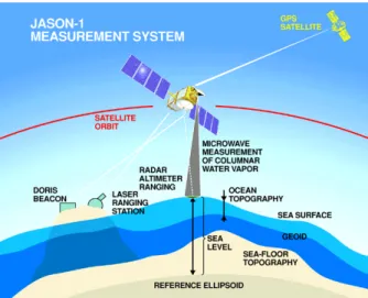
A satellite altimetry measure provides the following H= R + SSH + ∆h + e, (1) in which we have H as the satellite height (or altitude of the orbit) relative to the reference ellipsoid, R is the distance between the altimeter and the instantaneous sea surface, SSH is the sea surface height relative to the reference ellipsoid, ∆h is the instantaneous effect of the tide and e is the term associated with measurement errors and corrections. Figure 2 shows the satellite altimetry measurement principles.
Figure 2 – Satellite altimetry measurement scheme over the sea surface. The
The sea surface height is given by
SSH= N + SST, (2) where N is the geoid height and SST corresponds to the sea surface topography. In turn, SST has a quasi-stationary component, which can be considered stationary in position and magnitude over a long period of time and a time-dependent component, which evolves rapidly (Hwang, 1997). In this way, one can also obtain the geoid height by removing the two components of the dynamic topography from the SSH values (see Hwang et al., 2002).
DATA PROCESSING
Satellite altimetry data were obtained as Geophysical Data Records (GDR) (Cheney et al., 1991) or Ocean Products (OPR) (Dumont et al., 1995). The files come in binary/big-endian format (format used on workstations) and must be converted to ASCII to be read and edited. Data processing was performed in this study in the following order:
Step 1. We applied the geophysical corrections, provided in the
GDR and OPR, referring to each observation point to the raw data, including atmospheric refraction, sea-state bias, inverted barometer and ocean tidal height corrections (Chelton et al., 2001).
Step 2. After these corrections were applied, sea surface
height values were obtained for each satellite measurement point, with a total of 180, 422 points. The satellite tracks were then separated into ascending (86, 324 points) and descending (94, 098 points) passes.
Step 3. We obtained the along-track SSH directional derivatives,
namely, the sea surface gradients (SSG). The gradients are less affected by long-wavelength errors than the sea surface heights, in addition to emphasizing the features associated with the short-wavelengths of the SSH. Given the small separation between along-track points (between 3.3 and 7 km), the directional derivative is obtained by approximation by the slope of the line between two consecutive points
SSG(α) =SSH2− SSH1
d , (3)
where d is the distance between points, which should not exceed 2 seconds in time, or ∼15 km (Molina, 2009; Paolo & Molina, 2010). The geographic location of each SSG corresponds to the average location of the two SSHs used for its calculation.
For geodetic missions, the standard error associated with the data set can be evaluated by the altimeter noise level of each satellite (σ)(Hwang & Parsons, 1996):
σε2=σ 2 1+σ 2 2 d2 = 2σ2 d2 , (4)
where d is the mean along-track point spacing.
Step 4. Finally, the sea surface gradients were filtered by a
Gaussian filter to remove wavelengths shorter than 40 km, which were below the noise threshold. The data and results illustration and some processing were performed using the GMT (Generic Mapping Tools) package (Wessel & Smith, 1995).
OCEAN FLOOR TECTONIC FEATURES SIGNATURES
Most of the ocean floor features, depending on the extension, present a reproducible signature on a series of parallel profiles of the horizontal gradients of the gravity field (Royer et al., 1989). These gradients can be the SSG when considering the directional derivative of SSH along satellite tracks or the deflection of the vertical (DOV) when we consider the directional derivative of the geoid height.
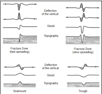
Figure 3 – Schematic signatures of the geoid and the deflection of the vertical
(horizontal derivative of the gravity field) associated with some tectonic features of the ocean floor: fracture zones, seamount and trough (adapted from Royer et al., 1989). The arrows indicate the direction of the satellite along-track.
Some examples of signatures of ocean floor features in the horizontal gradients of the gravity field are shown in Figure 3, other signatures can be found in Royer et al. (1989). The signature
of a fracture zone, for example, depends mainly on its spreading rate. Seamounts are recognized by two peaks, one positive and one negative, of the same amplitude. Aseismic ridges (such as the Rio Grande Rise) and plateaus are easily identifiable, but depending on their width and height relative to adjacent basins, it can be difficult to differentiate them.
Other factors such as the direction of the satellite tracks and the orientation of the tectonic features relative to the satellite ground track may also interfere with the feature signature, which may be identical or reversed on the ascending or descending track sets. In general, structures oriented north-south will present the same signatures, and east-west oriented features will have reverse signatures (Royer et al., 1989).
RESULTS AND DISCUSSION Sea Surface Height (SSH)
The structures identified through the SSH variations are positioned correctly in relation to the bathymetry of the region. However, it was observed that, in the Geosat ascending tracks, the sea surface height presents a discrepancy (shift) as compared to other satellites’ tracks. The same goes for ERS1 descending tracks. However, this does not affect sea surface gradients due to the continuous differentiation along tracks (Sandwell & Smith, 1997). Thus, the analysis of the SSH variations was performed for the ERS1 and Geosat missions separately, to avoid ”ghosts” that do not correspond to structures. The Seasat mission alone does not have enough tracks to characterize oceanic structures in the study area and therefore has not been analyzed. However, data from all three missions were used in the SSG calculation.
The variations of the sea surface height reveal some features of the ocean floor, such as the NW-SE trending rift, some fractures of the Rio Grande Fracture Zone and some larger seamounts (Fig. 4). The SSH values present differentiated responses to the ascending and descending sets of tracks.
The main structures that can be highlighted in the ascending track set (Figs. 4a and 4b) are the Rio Grande Fracture Zone and three seamounts. Although the shape of the Rio Grande Rise is not very visible, the SSH curves have their negative values corresponding to the rift trough.On the descending tracks (Figs. 4c and 4d), one can easily locate the two units of the rise (WRGR and ERGR). The two flanks and the central trough, which form its rift, correspond to positive and negative values of SSH, respectively. The fracture zone is also observed in this set of tracks and two seamounts are identified, with emphasis on a positive feature (27◦S and 38◦W) corresponding to a seamount
from the Jean Charcot seamounts. Adjacent to this feature, there are a series of tracks which SSH values present characteristic signatures of seamounts that do not have correspondents in the bathymetric map. In this way, it is possible that there are other seamounts of similar or smaller size than the one previously characterized (Jean Charcot) in this region.
Sea Surface Gradient (SSG)
Variations of sea surface gradients provide more details of the ocean floor structures than SSH values alone. In addition to the features already observed with SSH, several seamounts are more visible in the SSG curves. The positioning of the structures is very precise, but the proximity of some features can influence the response of the gradients, as well as the position of the satellite and the direction of the tracks in relation to these features. Therefore, it is important to consider the two sets of tracks in the SSG (and SSH) analysis, because they complement each other, since some structures can be observed in only one of the maps.
In the ascending and descending tracks maps with SSG filtered values (Fig. 5) it is possible to see that the SSG better emphasizes the lineaments around the Rio Grande Rise, making it possible to identify the Rio Grande Fracture Zone and a linear structure located below the WRGR corresponding to the Chuí Lineament.
The trough of the central rift of the rise is marked by positive and negative values of SSG in the ascending and descending tracks, respectively, that is, the two sets of tracks present reverse responses to this feature. A north-south trending structure that is not visible on the sea surface gradient maps is the Vema channel. As there is no significant difference in the SSG values between the channel and its surroundings, this feature does not stand out in these data.
In order to analyze the gradient responses according to the characteristic signatures of the tectonic features (according to Fig. 3), the SSG values should be plotted along the ascending and descending satellite tracks (Fig. 6). The joint analysis of the satellite tracks of the three altimetric missions is important because it makes the data more dense, providing a more complete information of the region of interest. However, it is interesting to separate the sets of ascending and descending tracks of each mission into subsets, trying to maintain a greater spacing between the tracks, which facilitates the visualization of smaller features, especially seamounts.
Figure 4 – (a) ERS1-GM and (b) Geosat-GM ascending and (c) ERS1-GM and (d) Geosat-GM descending profiles of the
sea surface height (SSH) plotted along the satellite ground tracks, with positive amplitude to the north (amplitude scale is 6 m per degree of longitude). Red lines indicate identified fracture zones and red circles denote seamounts. The rectangle indicates features that show no equivalent in bathymetry.
Figure 5 – (a) Ascending and (b) descending tracks from the three altimetric missions with filtered values of sea surface
Figure 6 – Sea surface gradients (SSG), plotted along (a) ascending and (b) descending tracks from the three missions.
Positive SSG values in relation to the track are represented in blue and negative values in red. The SSG amplitude scale is 250µrad per degree of longitude.
Figure 7 – Geographic location of an (a) ascending and a (c) descending track from ERS1-GM. Distribution of bathymetric and SSG values
along the (b) ascending and (d) descending pass. The seamounts are surrounded by the black circles.
Seamounts
Several seamounts and guyots can be observed by relating the SSG response with the 3500 m bathymetric contour. According to their signature on the sea surface gradients, seamounts are characterized by two opposing peaks of the same magnitude. In this way, the center of the seamount is positioned between the two
peaks (Figs. 7b and 7d). The amplitude of the two peaks may not be the same when there are other structures near the mount, and if it is very small.
In Figures 8 and 9, all the seamounts identified in the study area are highlighted. The SSG responses for the ascending and descending tracks differ from each other, and one set does not necessarily present the same seamounts and guyots pointed at the
Figure 8 – Seamounts identified on the SSG ascending tracks of the three satellite missions. The black lines mark the center of the seamount in frames a, b, c, d and e. The amplitude scale is 90µrad per degree of longitude fora, b, d and e, and 70µrad per degree of longitude forc.
Figure 9 – Seamounts identified on the SSG descending tracks of the three satellite missions. The black lines mark the center of the seamount in frames a, b, c, d and e. The amplitude scale is 90µrad per degree of longitude fora, b, d and e, and 70µrad per degree of longitude forc.
other. The possible features characterized by SSH with seamounts signatures are not identified in the gradient curves (Fig. 10). The proximity between these structures and adjacent ones could be influencing the SSG response making it difficult to distinguish the seamounts from the other tectonic features in these data.
Fracture Zone
Figure 11(b and d) shows the characteristic signature of the Rio Grande Fracture Zone in SSG. The fracture zones signatures in the gradients vary with the spreading rate, so we cannot correlate the lineations in the SSG data with the exact bathymetric location of
Figure 10 – (a) Bathymetry, (b) Geosat-GM SSH variations, and (c) Geosat-GM SSG variations of the region where the possible
features with characteristic signatures of seamounts, identified through SSH descending tracks, are located. The SSH amplitude scale is 3 m per degree of longitude and the SSG is 150µrad per degree of longitude.
Figure 11 – Geographic location of an (a) ascending and a (c) descending track from Geosat-GM. Distribution of bathymetric and SSG values along the (b) ascending
Figure 12 – Fracture zones identified in the ascending (left) and descending (right) tracks of SSG from the three satellites missions.
the fracture zones (Shaw & Cande, 1987). The satellite altimetry data can, however, predict the spreading direction by determining tectonic flow lines which are parallel to the fracture zones (Mayes et al., 1990).
Figure 12 shows some of the identified fractures in the eastern part of the Rio Grande Rise. The ascending and descending tracks present reverse responses to the fractures of east-west direction. The circled region (Fig. 12, frames b) corresponds to a fracture in the bathymetry, but its gradient signature is confused with that of adjacent seamounts, making it difficult to distinguish them with SSG data. In this case, the gradient response seems to be more related to the seamounts than to the fracture zone.
CONCLUSIONS
Sea surface height (SSH) and sea surface gradients (SSG) from the ERS1-GM, Geosat-GM and Seasat satellite altimetry data were both important for the identification and characterization of structures of the ocean floor. While SSH identifies larger structures, SSG also characterizes several smaller seamounts, by highlighting the short wavelengths of sea surface height.
Among the structural features observed with the SSH data are the Rio Grande Fracture Zone, few larger seamounts and the main structure of the Rio Grande Rise, its NW-SE trending rift that cuts the two units of the ridge. The sea surface gradients reveal the same oceanic structures as SSH, but in greater detail, such as the fractures to NE and SE of the rise and the Jean Charcot seamounts to NW of the RGR, as well as several others that were not visible in the SSH curves. The main structure of the rise itself presents a greater level of detail, such as seamounts in its highest region. It was also possible to highlight a linear structure corresponding to the Chuí Lineament, located to the south of the WRGR.
Both SSH and SSG correctly position the identified features in relation to the bathymetry of the site. However, sea surface height data show discrepancies related to the position of the identified structures, for some satellites. Therefore, when analyzing the tracks from these three satellites together, it is necessary to calculate this discrepancy and correct the SSH data that is displaced. This error will not affect the SSG data due to the calculation of the along-track directional derivative.
In the case of SSG, very close structures can alter the efficiency of their identification, making it difficult to characterize them. Other factors that also influence the response of the gradients are the direction of the satellite tracks and the orientation of the tectonic features in relation to the tracks. In this
way, ascending and descending tracks can show reverse results, or some structures can be observed in only one of the maps. Therefore, it is fundamental to always consider the two sets of tracks from various satellites. In addition, it is also important to analyze tracks with a greater spacing between them to facilitate the visualization of smaller details, especially seamounts that can go unnoticed in an overview with all the tracks in a single map.
The study allowed us to identify possible structures with a characteristic signature of seamounts, through the analysis of SSH tracks, which were not previously characterized in the literature and do not have corresponding in topographic/bathymetric models. Although there is no evidence of such features in the SSG curves, it is possible that there are other seamounts close to those already identified from the Jean Charcot seamounts. An important implication of the results obtained is that, with the use of other more recent, dense and accurate altimetric missions public data, there is a great chance to perform a good characterization of the existing features and eventually to identify new structures and characteristics of the region.
ACKNOWLEDGMENTS
This study was financed in part by the Coordenação de Aperfeiçoamento de Pessoal de Nível Superior - Brazil (CAPES).
REFERENCES
AMANTE C. 2009. ETOPO1 1 Arc-Minute Global Relief Model: Procedures, Data Sources and Analysis. http://www.ngdc.noaa.gov/ mgg/global/global.html. URL https://ci.nii.ac.jp/naid/20001162728/. BARKER PF. 1983. Tectonic evolution and subsidence history of the Rio Grande Rise. In: BARKER PF, CARLSON RL et al. (Eds.). Initial Reports of the Deep Sea Drilling Project. Volume 72, p. 953–976. US Government Printing Office, Washington, DC 20402-9325 USA.
CHELTON DB, RIES JC, HAINES BJ, FU LL & CALLAHAN PS. 2001. Chapter 1 Satellite Altimetry. In: FU LL & CAZENAVE A (Eds.). International Geophysics. Volume 69 of Satellite Altimetry and Earth Sciences, p. 1–ii. Academic Press. doi: 10.1016/S0074-6142(01)80146-7. URL http://www.sciencedirect.com/science/article/ pii/S0074614201801467.
CHENEY RE, DOYLE NS, DOUGLAS BC, AGREEN RW, MILLER L, TIMMERMAN EL & McADOO DC. 1991. The complete Geosat altimeter GDR handbook. NOAA Manual NOS NGS, 7: 77.
CONSTANTINO RR, HACKSPACHER PC, DE SOUZA IA & LIMA COSTA IS. 2017. Basement structures over Rio Grande Rise from gravity
inversion. Journal of South American Earth Sciences, 75: 85–91. doi: 10.1016/j.jsames.2017.02.005. URL http://www.sciencedirect.com/ science/article/pii/S0895981116302929.
DRAGOI-STAVAR D & HALL S. 2009. Gravity modeling of the ocean-continent transition along the South Atlantic margins. Journal of Geophysical Research Solid Earth, 114(B09401). URL http://dx.doi.org/ 10.1029/2008JB006014.
DUMONT JP, OGOR F & STUM J. 1995. Quality Assessment of Cersat Altimeter OPR Products 168-Day Repeat Period. French Processing and Archive Facility, Toulouse, France.
GAHAGAN LM, SCOTESE CR, ROYER JY, SANDWELL DT, WINN JK, TOMLINS RL, ROSS MI, NEWMAN JS, MÜLLER RD, MAYES CL, LAWVER LA & HEUBECK CE. 1988. Tectonic fabric map of the ocean basins from satellite altimetry data. Tectonophysics, 155(1-4): 1–26. GAMBOA LAP & RABINOWITZ PD. 1981. The Rio Grande fracture zone in the western South Atlantic and its tectonic implications. Earth and Planetary Science Letters, 52(2): 410–418. doi: 10.1016/0012-821X(81)90193-X. URL http://www.sciencedirect.com/science/article/ pii/0012821X8190193X.
GAMBOA LAP & RABINOWITZ PD. 1984. The evolution of the Rio Grande Rise in the southwest Atlantic Ocean. Marine Geology, 58(1): 35–58. doi: 10.1016/0025-3227(84)90115-4. URL http://www. sciencedirect.com/science/article/pii/0025322784901154.
HWANG C. 1997. Analysis of some systematic errors affecting altimeter-derived sea surface gradient with application to geoid determination over Taiwan. Journal of Geodesy, 71(2): 113–130. doi: 10. 1007/s001900050080. URL https://doi.org/10.1007/s001900050080. HWANG C, HSU HY & JANG RJ. 2002. Global mean sea surface and marine gravity anomaly from multi-satellite altimetry: applications of deflection-geoid and inverse Vening Meinesz formulae. Journal of Geodesy, 76(8): 407–418.
HWANG C & PARSONS B. 1996. An optimal procedure for deriving marine gravity from multi-satellite altimetry. Geophysical Journal International, 125: 705–718. doi: 10.1111/j.1365-246X.1996.tb06018. x. URL http://adsabs.harvard.edu/abs/1996GeoJI.125..705H. KIM SS & WESSEL P. 2011. New global seamount census from altimetry-derived gravity data. Geophysical Journal International, 186(2): 615–631.
LEYDEN R, LUDWIG WJ & EWING M. 1971. Structure of continental margin off Punta del Este, Uruguay, and Rio de Janeiro, Brazil. AAPG Bulletin, 55(12): 2161–2173.
MARKS KM & SMITH WHF. 2007. Some remarks on resolving seamounts in satellite gravity. Geophysical Research Letters, 34:L03307(3). doi:10.1029/2006GL028857.
MAYES CL, LAWVER LA & SANDWELL DT. 1990. Tectonic history and new isochron chart of the south Pacific. Journal of Geophysical Research: Solid Earth, 95(B6): 8543–8567. doi: 10.1029/JB095iB06p08543. URL https://agupubs.onlinelibrary.wiley.com/doi/abs/10.1029/ JB095iB06p08543.
MOHRIAK WU, NÓBREGA M, ODEGARD ME, GOMES BS & DICKSON WG. 2010. Geological and geophysical interpretation of the Rio Grande Rise, south-eastern Brazilian margin: extensional tectonics and rifting of continental and oceanic crusts. Petroleum Geoscience, 16(3): 231–245. MOLINA EC. 2009. O uso de dados de missões geodésicas de altimetria por satélite e gravimetria marinha para a representação dos elementos do campo de gravidade terrestre. Ph.D. thesis. Tese de livre docência, Departamento de Geofísica, IAG-USP, Universidade de São Paulo, São Paulo, Brazil. 100 pp.
NASA/JPL-Caltech. 2010. Ocean Surface Tophography from Space. Gallery. Jet Propulsion Laboratory, California Institute of Technology. Available on: https://sealevel.jpl.nasa.gov/gallery/posters/?ImageID= 10. Access on: November 12th, 2018.
O’CONNOR JM & DUNCAN RA. 1990. Evolution of the Walvis Ridge-Rio Grande Rise Hot Spot System: Implications for African and South American Plate motions over plumes. Journal of Geophysical Research: Solid Earth, 95(B11): 17475–17502. doi: 10.1029/JB095iB11p17475. URL https://agupubs.onlinelibrary.wiley.com/doi/abs/10.1029/ JB095iB11p17475.
PAOLO FS & MOLINA EC. 2010. Integrated marine gravity field in the Brazilian coast from altimeter-derived sea surface gradient and shipborne gravity. Journal of Geodynamics, 50(5): 347–354.
PESSOA JCDO. 2015. Estudo mineralógico e geoquímico de crostas polimetálicas (Fe-Mn-Co) das áreas Alpha e Bravo da Elevação do Rio Grande. Master’s thesis. Universidade Estadual de Campinas, São Paulo, Brazil. URL http://repositorio.unicamp.br/jspui/handle/REPOSIP/ 304754. 83 pp.
ROHDE JK, VAN DEN BOGAARD P, HOERNLE K, HAUFF F & WERNER R. 2013. Evidence for an age progression along the Tristan-Gough volcanic track from new40Ar/39Ar ages on phenocryst phases. Tectonophysics,
604: 60–71.
ROYER JY, GAHAGAN L, LAWVER LA, MAYES CL, NURNBERG D, SANDWELL DT & SCOTESE CR. 1990. A Tectonic Chart for the Southern
Ocean Derived from Geosat Altimetry Data. chapter 7. AAPG Special Volumes.
ROYER JY, SCLATER JG & SANDWELL DT. 1989. A preliminary tectonic fabric chart of the Indian Ocean. Proceedings of the Indian Academy of Sciences-Earth and Planetary Sciences, 98(1): 7–24.
SANDWELL DT & SMITH WH. 1997. Marine gravity anomaly from Geosat and ERS 1 satellite altimetry. Journal of Geophysical Research-Solid Earth, 102: 10039–10054. doi: 10.1029/96jb03223. SHAW PR & CANDE SC. 1987. Shape and amplitude analysis of small-offset fracture zone geoid signals. Eos, Transactions American Geophysical Union, 68(44): 1462.
USSAMI N, CHAVES CAM, MARQUES LS & ERNESTO M. 2012. Origin of the Rio Grande Rise–Walvis Ridge reviewed integrating palaeogeographic reconstruction, isotope geochemistry and flexural modelling. Geological Society, London, Special Publications, 369(1): 129–146.
WESSEL P, MATTHEWS KJ, MüLLER RD, MAZZONI A, WHITTAKER JM, MYHILL R & CHANDLER MT. 2015. Semiautomatic fracture zone tracking. Geochemistry, Geophysics, Geosystems, 16: 2462–2472. doi:10.1002/2015GC005853.
WESSEL P & SMITH WH. 1995. New version of the generic mapping tools. Eos, Transactions American Geophysical Union, 76(33): 329.
Recebido em 9 abril, 2018 / Aceito em 7 novembro, 2018 Received on April 9, 2018 / accepted on November 7, 2018