THE VALUATION OF CALLABLE DEFAULTABLE BONDS
William Hilebrand
Project submitted as partial requirement for the conferral of Master in Finance
Supervisor:
Prof. João Pedro Vidal Nunes, Associate Professor, ISCTE Business School, Department of Finance
I
Abstract
The present work studies the valuation of callable defaultable bonds, when firm value and interest rate are both stochastics. When valuing long term contingent claims which underlying asset is a bond, it is important to assume endogenous bankruptcy risk since, in the long run, firm value and interest rate might not walk together. The firm value is described by an one-factor geometric Brownian motion and the interest rate follows an one-factor square root process.
This study presents sensitivity analysis on yield spreads and option values with variations on host bond prices and interest rate volatilities. Furthermore, three different assumptions to model the interest rate behaviour (the CIR model, the Vasicek model and a constant interest rate) will be compared, in order to find significant differences and try to understand which one fits better to the theory.
Key words: Callable bonds, stochastic interest rate, CIR model, Black-Scholes-Merton
model.
II
Resumo
O presente trabalho debruça-se sobre a avaliação de obrigações callable com risco de falência, quando o valor da empresa e a taxa de juro são ambos estocásticos. Quando se avalia direitos contingentes de longo prazo cujo activo subjacente é uma obrigação, torna-se importante considerar o risco de falência como variável endógena visto que, no longo prazo, o valor da empresa e a taxa de juro podem não ter o mesmo comportamento. O valor da empresa é explicado por um movimento Browniano geométrico de um só factor e a taxa de juro segue um processo de raíz quadrada, também de um só factor.
Este estudo apresenta análises de sensibilidade do spread das yields e do valor das opções, para variações no preço da obrigação subjacente e na volatilidade da taxa de juro. Serão também comparados três pressupostos diferentes para o comportamento da taxa de juro (modelo CIR, modelo Vasicek e taxa de juro constante), de forma a encontrar diferenças relevantes e perceber qual deles se adequa melhor à teoria.
Palavras-chave: Obrigações Callable, taxa de juro estocástica, modelo CIR, modelo
Black-Scholes-Merton.
III
Acknowledgments
I’m entirely grateful to my supervisor, Prof. João Pedro Nunes, for all the helpful comments and orientation which were determinant to the accomplishment and success of this thesis.
My appreciations are also reserved to my brother, Wesley Hilebrand, for his constructive comments and positive discussions; to my parents and closest friends for their incredible support.
IV
Contents
1. Introduction ... 1
2. Related Literature ... 3
3. Callable Defaultable Bond ... 6
3.1. Definition ... 6
3.2. Behaviour and Rational ... 7
3.3. Stochastic Models ... 7 3.4. Theoretical pricing ... 10
4. Valuation Methods ... 12
4.1. Yield-to-worst... 12 4.2. Binomial Lattice ... 145. Numerical results ... 20
5.1. Under the CIR model assumption ... 20
5.2. Comparison ... 24
6. Conclusion ... 29
Bibliography ... 31
Appendix A ... 33
A.1. Inputs ... 33
A.2. Import data function ... 33
A.3. Callable defaultable bond value et al. under CIR model ... 34
A.4. Callable defaultable bond value et al. under Vasicek model ... 46
1
Chapter 1
Introduction
When firm’s capital structure and financing decisions are required, two theories rise to the surface trying to answer which combination of equity and debt maximize the value of a company or if a company needs external finance, which one shall be the best way.
Based on the Pecking Order Theory, if external finance is required, firms prefer issuing debt over equity. Markets tend to believe that, when firms issue equity their stocks are overpriced, which means, they issue equity in order to benefit from the gap between the market stock price and its fair price. When raise equity occurs, usually the stock price falls down. Instead, firms can issue debt and take advantage of the tax shield, avoiding any disturb on the firm’s market value.
However, the Trade-off Theory says that the previous effect does not hold all the time. What really matters is the comparison between its marginal benefit and its marginal cost. Usually when firms have a low financial leverage ratio they issue debt because, on one hand, they can deduct the cost of debt on the taxable profit (tax shield) and, on the other hand, they are not so affected by financial distress (caused mainly by bankruptcy cost), which means, the marginal benefit given by the tax shield is greater than the incremental cost of financing, caused by bankruptcy costs. Until now, all arguments support the same conclusion as the
Pecking Order Theory. The disagreement exists when firms are on the financial distress
region, where the marginal cost tends to increase substantially, compared to the marginal benefit.
The main conclusion for a firm with normal leverage is that debt is the consensual source of financing; typically bonds, as a financial and tradable instrument, are very often used. As referred by Duffie and Singleton (1999), and also confirmed by Bloomberg data analysis, “The majority of dollar-denominated corporate bonds are callable”, we agree on the relative importance of this type of corporate debt in the financial market. Therefore, this thesis proposes to develop a deeper study on the valuation of callable defaultable bonds, researching
2
the approaches already developed, verifying the computational tractability of a particular method and testing different stochastic diffusion processes for the risk-free interest rate.
Thus, the central topic of this thesis stands on the numerical implementation of the method suggested by Acharya and Carpenter (2002), and exposed in appendix B. In addition, it also analyses the sensitivity of the call and default features embedded to the host bond, as well as, some comparisons under different stochastic processes for the interest rate.
This thesis will be structured as follows. Chapter 2 shows the reference progress regarding the study of callable bonds. Chapter 3 presents the definition and behaviour of callable defaultable bonds, as well as the stochastic models which this thesis will be based on. Chapter 4 describes two approaches to the valuation of callable defaultable bonds. Chapter 5 presents numerical results regarding callable defaultable bonds valuation and some comparisons with different stochastic diffusion processes for interest rate, namely the Vasicek (1973) model. Finally, Chapter 6 summarizes the most important conclusions derived from this work.
3
Chapter 2
Related Literature
Since many authors have been applying theirs studies to the callable bond and callable defaultable bond valuation, several references, in the financial literature, can be found.
Black and Scholes (1973) and Merton (1974) were not the pioneers of option and default risk pricing but they gave an important contribution to these themes, specially developing a theoretical valuation formula for call and put options on the stock price under an arbitrage-free market and with some more realistic assumptions. Merton (1974) presented a model capable of estimating the risk-neutral probability of firm default and of pricing bonds, as well as its credit spread. He assumed that the return on asset of the company follows a lognormal distribution, with expected value and volatility of the assets estimated using an approach suggested by Jones, Mason and Rosenfeld (1984). Hull, Nelken and White (2004) improved the approach of Merton (1974) by presenting an alternative way to estimate the parameters of the model, and by adding a deeper insight into the linkages between the credit market and the options market.
Brennan and Schwartz (1977) extend the work developed by Black and Scholes (1973) and Merton (1974) to the pricing of convertible bonds. The valuation of this financial instrument is quite complex because there are two options embedded into the bond: one is owned by the firm issuer and the other is owned by the investor. Consequently, the exercise decisions are dependent one each other. However, these authors only assumed a stochastic diffusion process to the firm value and the risk-free interest rate is constant through time. In fact, due to the boundary conditions imposed, there is no reduced-form to value the convertible bond and, thus they resort to numerical methods to solve it.
The traditional structural approach for valuing simple and more complex bonds with call and default features typically treats interest rate as constant and assumes a stochastic process for the firm’s assets value. Then the optimal call policy and, consequently, the bond value is determined by minimizing the present value of future liabilities. Duffie and Singleton
4
(1999) and Jarrow, et al. (2006) developed a new valuation approach, based on a reduced-form model for pricing contingent claims subject to default risk. They do not consider the firm’s asset value as the explanatory variable; instead, they consider the interest rate as the explanatory one, to the bond valuation. Duffie and Singleton (1999) measured the default risk through an hazard-rate and an expected fractional loss that are exogenous1, which means that they only consider the interest rate as the stochastic variable. The added value of this paper is the parameterization of losses at default in terms of fractional reduction in market value that occurs at default. Jarrow, et al. (2006) also followed the approach developed by Duffie and Singleton (1999). They present an improvement since they introduce the information about firm’s assets and capital structure, and improve the tractability as long as they can capture some differences between call and default decisions. They all present the valuation of callable defaultable bonds.
When long-term contingent claims need to be priced, there are a few methods that can give an accurate answer or support theories about the behaviour of those contingent claims. These were the main incentives for Acharya and Carpenter (2002) to present an alternative and more complex valuation approach. They were the first ones to present a valuation method for coupon-bearing corporate debts that incorporates both stochastic interest rates and endogenous bankruptcy. It gives degrees of freedom to capture the individual behaviour of each embedded option, but the computational tractability gets harder because it requires a two-dimensional lattice tree. They also show the hedging strategies under such conditions and the implications of the exogenous bankruptcy assumption.
The papers enumerated until now were all developed under one-factor models, Gaussian or non-Gaussian. The literature on principal component analysis shows that three is the optimal number of factors to model interest rates, taking into account the trade-off between accuracy and manageability. Of course, the Gaussian models are easier to deal with, due to the vast properties that the normal distribution has but they can yield negative interest rates. Nevertheless, multifactor term structure models are only tractable when we are pricing vanilla bonds. For more complex bonds there is no closed-form solution and its computational implementation is really arduous. This is why there are only a few papers using models with
5
more than one factor. Longstaff and Schwartz (1992) is an example of a multifactor model. They actually use a two-factor model, a generalization of the CIR model.
6
Chapter 3
Callable Defaultable Bond
3.1. Definition
A callable defaultable bond is simply a bond with an embedded call option.
For a deeper insight about the instrument’s concept, let’s split and clarify all this terms. A straightforward definition for a bond could be cited from Brealey and Myers (2003): “A bond is simply a long-term debt. If you own a bond, you receive a fixed set of cash payoffs:
Each year or semester until the bond matures, you collect an interest payment, then at maturity, you also get back the face value of the bond, known as principal”. The interest
payment is named coupon, and the only type of bond that doesn’t pay it is the zero coupon bond. Actually, the bond has an invisible embedded option owned by the bond issuer, the default option. The default option can be triggered whenever the firm is not able to payback the outstanding debt. For this reason, the vanilla bond is sometimes named as defaultable bond. When firms issue bonds, they can also embed an option of earlier reimbursement, i.e., they establish a schedule of dates (or periods) and strike prices when they decide if they redeem or not the debt. These bonds are commonly known as callable (defaultable) bonds.
Now it’s understandable if we re-define a callable defaultable bond as a bond that can be redeemed or defaulted before its maturity date, and if so, the issuer must payback the outstanding amount or, in case of default, the insolvency firm value to the bond holder.
To avoid any doubts, I will not make any difference between firm and issuer. Both represent the same agent and risk. The firm will be the one who will issue the bond (without loss of generality). The host bond terminology, mentioned ahead, refers to the non-defaultable and non-callable bond whose options are linked to. While the plain vanilla bond or just vanilla bond is a defaultable bond without any more options embedded.
7
3.2. Behaviour and Rational
Every day firms are challenged with new financial problems and, usually, they look for financial institutions services to solve them. This is the reason why new financial instruments are created and modified and, consequently, financial markets become even more complex. Certainly a callable defaultable bond was not an exception and it must have been created to face firms’ needs.
The firm can have several incentives to issue a callable defaultable bond. On the one hand, a defaultable bond (opposing to the non-defaultable bond) is desired because the firm doesn’t have to allocate collaterals in order to guarantee the full debt services and, in case of default, the firm pays only the insolvency value to the bond holder. On the other hand, a callable bond is an hedging instrument because it protects the firm against the interest rate downward move, i.e., the issuer has the right to payback the outstanding debt before its maturity by a pre-determined price in case the interest rate falls. If it happens, the firm will have the opportunity to issue a new bond at a lower coupon rate (lower cost).
The investors view point is always a trade-off between return and risk. It’s a matter of expectations. The principal incentive for investors to buy this type of bond is the lower price compared to the vanilla bond (nevertheless riskier). This discount is due to two disadvantages: the first one is the possibility of earlier redemption, that is, if investors have a fixed investment horizon, in case of earlier redemption, they will have to invest in another bond with lower coupon rate compared to the previous one (achieving a lower yield to maturity); the last one is a consequence of a peculiarity of the callable defaultable bond, which means, when interest rate falls, the price will not increase at the same proportion as the vanilla bond. This feature is denoted by negative convexity.
3.3. Stochastic Models
As mentioned before, the principal idea of this thesis is to evaluate a callable bond in which the issuer has the possibility to default, also denoted by callable defaultable bond.
8
In order to evaluate the bond as realistic as possible, two stochastic processes will be considered to model the variables: one for the firm’s asset value, 𝑉, and another for the instantaneous interest rate, 𝑟. The interest rate process will be useful to evaluate the bond and the call provision whereas the firm’s asset value process will be useful to determine the default risk.
Let’s assume that the firm has a single bond outstanding (without loss of generality) that pays a fixed continuous coupon c and matures in T years and that the value of the firm is equal to the value of its assets. Suppose also that investors are price takers and cannot influence, individually, the firm value and the market conditions. Additionally, let’s assume they can trade continuously in a complete and frictionless market. As a result, there exists a martingale measure 𝑄 under which the expected rate of return on all assets at time 𝑑 conditionally to the 𝜎-algebra, ℱ𝑡, is equal to the instantaneous interest rate, 𝑟𝑡.
The stochastic model, created by Black and Scholes (1973) and improved by Merton (1974), tries to explain the behaviour of the firm value. This model is well known and widely accepted at the financial market due to its realistic assumptions and its goodness of fit when applied to the real financial world. Hence, the firm’s asset value will evolve according to the Black-Scholes-Merton’s model
𝑑𝑉𝑡
𝑉𝑡 = (𝑟𝑡− 𝛾𝑡)𝑑𝑑 + 𝜙𝑡𝑑𝑊�𝑡 , (1)
where 𝑊� is a Brownian motion under measure 𝑄, 𝛾𝑡 is the continuous dividend yield, 𝛾𝑡 ≥ 0, and 𝜙𝑡 is the diffusion factor, also called the volatility of returns, 𝜙𝑡 > 0.
There are many classes of stochastic models regarding interest rate behaviour and rationales to use each of them. In this thesis, two different models will be compared: the CIR model used by Acharya and Carpenter (2002) and the Vasicek (1977) model. Both are one-factor models. The reasons were briefly referred before nevertheless it’s important to note that the valuation of callable defaultable bond considering two diffusion processes with one-factor is already computationally arduous. Therefore and since no one developed yet an alternative method to implement the two diffusion processes with more than one factor through a tractable procedure, I will preserve the one-factor interest rate model.
9
The model developed by Cox, Ingersoll and Ross (1985) solves the serious problem regarding the negative values that the interest rate can assume in the Gaussian models. This feature has no economic or financial explanation, that is, no one is willing to pay to someone else to postpone his or her consumption into the future. People have preference to consume now instead of waiting to consume in the future. That is why Cox, Ingersoll and Ross (1985) suggest a nonnegative one-factor diffusion model (the CIR model, hereafter)
𝑑𝑟𝑡= 𝜅(𝜇 − 𝑟𝑡)𝑑𝑑 + 𝜎�𝑟𝑡𝑑𝑍�𝑡 , (2)
where 𝑍� is a Brownian motion under measure 𝑄, 𝑑〈𝑊� , 𝑍�〉𝑡 = 𝜌𝑡𝑑𝑑 is the instantaneous correlation, 𝜌𝑡 ∈ (−1,1), 𝜇 is the long-term value for the interest rate, 𝜇 > 0, 𝜅 is the speed of adjustment to the long-term value, 𝜅 > 0, and 𝜎 is the diffusion coefficient that determines the volatility of the process. It’s imposed that 2𝜅𝜇 > 𝜎2 to make sure that the upward drift is sufficiently large to make the negative values inaccessible.
The CIR model has important empirical properties that defend its utility: (i) Interest rates are always nonnegative. (ii) If the interest rate reaches to zero, it can subsequently become positive. (iii) When interest rate increases, the absolute variance of the interest rate increases as well. (iv) Interest rate has a recognized probability density function associated to the non-central chi-square.
The Vasicek (1977) model is the most tractable one but it doesn’t reflect the true economic behaviour of interest rates, and so, we expect that the Vasicek (1977) model gives worse results than the CIR model. This will be a topic to be analysed: if the marginal error for using the Vasicek (1977) model is worth the less effort to use it. Thus, the Vasicek (1977) diffusion process (the Vasicek model, hereafter) is expressed as follow:
𝑑𝑟𝑡 = 𝑎(𝑏 − 𝑟𝑡)𝑑𝑑 + 𝜎𝑑𝑍�𝑡 , (3)
where 𝑎 is the speed of mean reversion, 𝑏 is the long term value for the interest rate and 𝜎 is the instantaneous volatility.
10
3.4. Theoretical pricing
In a complete market it is straightforward to value a vanilla bond because the term structure is well-known. Also, all features of a vanilla bond as cash payoffs and its maturity dates are known allowing the exactly valuation (ignoring the uncertainty regarding firm’s default). However for a callable defaultable bond we don’t surely know when the bond will be redeemed. The future movements of interest rates can activate the call option or combined with firm value can activate the default option embedded to the bond, and consequently change the bond maturity as well as its fair price.
In order to go deeper into the callable defaultable bond understanding and analyse the interaction between call provision and default risk, I will consider two other types of bonds: a pure callable bond that is the non-defaultable bond with the same coupon, maturity and call provision, and a pure defaultable bond that is the non-callable bond with the same coupon, maturity and issuer.
When a bond has an option, we can comprehend its value in an alternative way. For instance, the value of a pure defaultable bond is the value of the host bond minus the default option value. Similarly, the value of a pure callable bond is the value of the host bond minus the call option value, and the value of a callable defaultable bond is the value of the host bond minus the call and default option value.
The host bond price at time 𝑑 is a function of the instantaneous interest rate,
𝑃𝑡 = 𝐸� �𝑐 � 𝛽𝑡,𝑠𝑑𝑠 𝑇 𝑡 + 1 ∙ 𝛽𝑡,𝑇� ℱ𝑡� , (4) where 𝛽𝑡,𝜏 = 𝑒− ∫ 𝑟𝑠𝑑𝑠 𝜏 𝑡 (5)
11
The optimal option value at time 𝑑 is
𝑓𝑥(𝑉𝑡, 𝐾𝑡, 𝑑) = sup
𝑡≤𝜏≤𝑇𝐸� �𝛽𝑡,𝜏�𝑃𝜏− 𝜅(𝑉𝜏, 𝐾𝜏, 𝜏)� +
� ℱ𝑡� , (6)
where 𝑥 identifies the evaluated option which can be the default option, the call option or the default plus call option, and the strike price, 𝜅, depends on the option in study, i.e.
𝜅(𝑣𝑡, 𝑘𝑡, 𝑑) = �
𝑣𝑡 𝑖𝑓 𝑥 = 𝑑𝑒𝑓𝑎𝑢𝑙𝑑 𝑜𝑝𝑑𝑖𝑜𝑛 𝑘𝑡 𝑖𝑓 𝑥 = 𝑐𝑎𝑙𝑙 𝑜𝑝𝑑𝑖𝑜𝑛 min(𝑣𝑡, 𝑘𝑡) 𝑖𝑓 𝑥 = 𝑐𝑎𝑙𝑙 + 𝑑𝑒𝑓𝑎𝑢𝑙𝑑 𝑜𝑝𝑑𝑖𝑜𝑛
(7)
Therefore, the equilibrium value for each bond is
12
Chapter 4
Valuation Methods
I will enumerate two distinct valuation methods. A deterministic one that assumes complete information about the future values of the variables. The second one is a stochastic approach that assumes a certain stochastic model associated to a particular probability distribution in order to explain the variables’ behaviour. Of course, the first one is straightforward because we have the full market information and know the future scenario, which means that, at the valuation moment, any financial instrument can be priced with certainty. However, the evidence shows that hardly ever the forward rates (or prices) coincide with the future spot rates; moreover, the future spot rates cannot be predicted with certainty. That is why the stochastic approach comes to light. It appears to improve the (weak) goodness of fit that the deterministic approach entails. In spite of the uncertainty embedded in the stochastic model, under certain conditions and probability distributions, it’s possible to find easily a closed form to price the financial contingent claim.
Next, I will present two different valuation methods, one to each valuation approach announced above. The Yield-to-worst that fits the deterministic approach and the binomial tree which is a general method able to fit both approaches; however, we will only use it for the stochastic approach.
4.1. Yield-to-worst
A traditional and antiquated approach for the valuation of a callable defaultable bond is the yield-to-worst. This is fairly popular amongst investors because it is a friendly measure of potential return that investors can earn. This is, however, an ex ante measure, i.e., at the end of the investment horizon, the effective return can be different from the initial one. This measure assumes the investor will hold the bond until the redemption date, the firm won’t
13
default and the term structure of interest rates will keep unchanged, i.e., the forward rates will be effectively the future spot rates.
The yield-to-worst is the lowest yield that an investor can earn, given all possible dates that the issuer can call the bond. To illustrate the traditional valuation method, let’s consider the following example:
Example 1
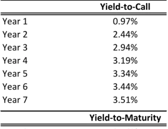
A callable defaultable bond, which matures in 8 years, bearing an annual coupon of 4%, is trading at 103. The bond is annually callable after 3 years. The yield curve that reflects the firm’s risk is the following: 1-year: 0.97%; 2-year: 2,47%; 3-year: 2.98%; 4-year: 3.23%; 5-year: 3.39%; 6-year: 3.49; 7-year: 3.56% and 8-year: 3.62.
We present below the Yields-to-Call and the Yield-to-Maturity, but the yields-to-call until year 2 are not feasible. The yield-to-call is the return that an investor can earn if the bond is called at the call date and the investor holds the bond until there. For instance, if the firm called the bond after 5 years, the investor would achieve a return of 3.34%. As the investor knows that the firm has the call provision and they will choose the call date that minimizes the firm’s cost, his potential rate of return will be 2.94%, also called yield-to-worse.
Table 1: The yield-to-call and yield-to-maturity for
a callable defaultable bond with coupon rate of 4% that matures in 8 years and is trading at 103
Yield-to-Call Year 1 0.97% Year 2 2.44% Year 3 2.94% Year 4 3.19% Year 5 3.34% Year 6 3.44% Year 7 3.51% Yield-to-Maturity Year 8 3.56%
14
In general and considering a yield curve with an upward slope shape, if the bond is traded below the par, its yield-to-worse will be the yield-to-maturity. However, if the bond is traded above the par, its yield-to-worse will be the earliest possible one. Practically, the callable bond price will be adjusted to yield the return demanded by investors.
4.2. Binomial Lattice
The binomial lattice has been widely used for pricing financial instruments and also real options due to the flexibility to adjust parameters and replicate portfolios. In addition, it’s easy to increase the calculus precision by increasing the time-steps, i.e., at the limit the binomial lattice converges to continuous time (of course, limited to the computational capacity).
To simplify the computational implementation, I will use a recombining binomial lattice. In fact, as we are dealing with two correlated stochastic processes, we cannot reproduce the trees directly and independently. The presence of two correlated stochastic processes implies to work with two-dimensional binomial lattice (or one-dimensional
quadrinomial lattice). The construction of the two binomial lattices requires attention because
there is a common factor that affects the values of those two processes, i.e., there is cross-variation between processes. For this reason, a specific methodology will be adopted, that is, mathematical transformations will be used in order to orthogonalize the diffusion factors of the processes and then, allow an easier construction of the trees. Even with the orthogonalized processes, the stochastic models won’t be totally independent because, as Acharya and Carpenter (2002) affirm, the intensity of the up and down moves is sensitive to the state of the variables. Nevertheless, the transformations simplify the construction of the variables’ trees.
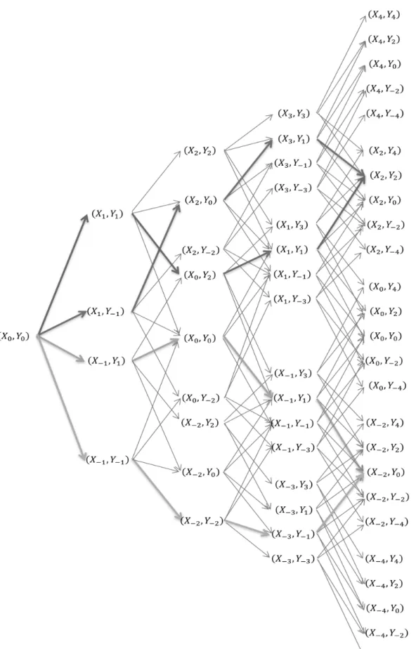
Figure 1 illustrates a possible binomial tree for two correlated variables with just 4 time-steps. In each node, the variables can move only one level up or down: (up-up, up-down, down-up, down-down).
15
16
The first step will be transforming the two state variables (𝑟𝑡 and 𝑉𝑡) into new diffusion processes that have constant volatility.
Let’s consider two transformations,
𝐺𝑡= ln(𝑉𝜙 𝑡)
𝑡 𝐻𝑡 = 2�𝑟𝑡
𝜎 (9)
Using Itô’s Lemma,2
𝑑𝐺𝑡 = 1 𝑉𝑡𝑑𝑉𝑡+ 12�− 1 𝑉𝑡� 𝑑〈𝑉, 𝑉〉𝑡 𝜙𝑡 = (𝑟𝑡− 𝛾𝑡)𝑑𝑑 + 𝜙𝑡𝑑𝑊�𝑡− 12𝜙𝑡2𝑑𝑑 𝜙𝑡 = �𝑟𝑡− 𝛾𝑡− 12𝜙𝑡 2� 𝜙𝑡 𝑑𝑑 + 𝑑𝑊�𝑡 𝑑𝐻𝑡 = 1 �𝑟𝑡𝑑𝑟𝑡+ 12�− 1 2𝑟𝑡32� 𝑑〈𝑟, 𝑟〉𝑡 𝜎 = 𝜅(𝜇 − 𝑟𝑡)𝑑𝑑 + 𝜎�𝑟𝑡𝑑𝑍�𝑡 𝜎�𝑟𝑡 − 1 4 � 𝜎2𝑟 𝑡𝑑𝑑 𝜎𝑟𝑡32 � = 𝜅𝜇 − 𝜎 2 4 − 𝜅𝑟𝑡 𝜎�𝑟𝑡 𝑑𝑑 + 𝑑𝑍�𝑡
we get two new diffusion processes that have constant and unity instantaneous volatility:
𝑑𝐺𝑡= 𝜇𝑡𝑑𝑑 + 𝑑𝑊�𝑡 , 𝜇𝑡 = 𝑟𝑡− 𝛾𝑡− 𝜙𝑡 2 2 𝜙𝑡 𝑑𝐻𝑡 = 𝜈𝑡𝑑𝑑 + 𝑑𝑍�𝑡 , 𝜈𝑡= 𝜅𝜇 − 𝜎4 − 𝜅𝑟2 𝑡 𝜎�𝑟𝑡 (10)
The second and last step consists in transforming the new processes (𝐺𝑡 and 𝐻𝑡) into uncorrelated diffusion processes. Therefore, let’s use the following transformations,
2
𝑑𝐹(𝑋𝑡, 𝑑) =𝜕𝐹𝜕𝑡𝑑𝑑 +𝜕𝑋𝜕𝐹𝑡𝑑𝑋𝑡+𝜕
2𝐹
17
𝑋𝑡 = 𝐺𝑡 𝑌𝑡 = 1
�1 − 𝜌𝑡2(−𝜌𝑡𝐺𝑡+ 𝐻𝑡) (11)
Using only algebra’s properties, we easily find the desired uncorrelated diffusion processes with constant instantaneous variation,
𝑑𝑌𝑡 = − 𝜌𝑡 �1 − 𝜌𝑡2 𝑑𝐺𝑡+ 1 �1 − 𝜌𝑡2 𝑑𝐻𝑡⟺ ⟺ 𝑑𝑌𝑡 = − 𝜌𝑡 �1 − 𝜌𝑡2 �𝜇𝑡𝑑𝑑 + 𝑑𝑊�𝑡� + 1 �1 − 𝜌𝑡2 �𝜐𝑡𝑑𝑑 + 𝑑𝑍�𝑡� ⟺ ⟺ 𝑑𝑌𝑡= 1 �1 − 𝜌𝑡2(−𝜌𝑡𝜇𝑡+ 𝜐𝑡) + 1 �1 − 𝜌𝑡2�−𝜌𝑑𝑊�𝑡+ 𝑑𝑍�𝑡� ⇒ ⇒ 𝑑𝑌𝑡 = 𝜇𝑡−𝑑𝑑 + 𝑑𝐵�𝑡 , (12) where 𝜇𝑡− = 1 �1−𝜌𝑡2 (−𝜌𝑡𝜇𝑡+ 𝜈𝑡) and 𝑑𝐵�𝑡= 1 �1−𝜌𝑡2 �−𝜌𝑑𝑊�𝑡+ 𝑑𝑍�𝑡�, and, 𝑑𝑋𝑡 = 𝜇𝑡+ 𝑑𝑑 + 𝑑𝑊�𝑡 , (13) where 𝜇𝑡+ = 𝜇𝑡
Once we get there, it´s easy to go backward into 𝑟𝑡 and 𝑉𝑡, by just using the inverse transformations:
𝑉𝑡 = 𝑒𝜙𝑡𝑋𝑡 𝑟𝑡 = �𝜎2 ��1 − 𝜌𝑡2𝑌𝑡+ 𝜌𝑡𝑋𝑡�� 2
(14)
Given the uncorrelated processes, we are almost ready to construct the binomial trees. Beforehand, we need to discretize the processes to make the binomial lattice possible.
18
Let’s consider a time-interval [0, 𝑇] and divide it into 𝑁 equal sub-intervals of length Δ𝑑. Additionally, let (𝑋𝑡, 𝑌𝑡) define the state of the variables, 𝑋 and 𝑌, at time 𝑑 which can evolve to four possible nodes, (𝑋𝑡+1+ , 𝑌𝑡+1+ ), (𝑋𝑡+1+ , 𝑌𝑡+1− ), (𝑋𝑡+1− , 𝑌𝑡+1+ ) and (𝑋𝑡+1− , 𝑌𝑡+1− ), where
𝑋𝑡+1+ = 𝑋𝑡+ (2𝑘1+ 1)√Δ𝑑 , 𝑋𝑡+1− = 𝑋𝑡+ (2𝑘1− 1)√Δ𝑑 𝑌𝑡+1+ = 𝑌𝑡+ (2𝑘2+ 1)√Δ𝑑 , 𝑌𝑡+1− = 𝑌𝑡+ (2𝑘2− 1)√Δ𝑑
(15)
and 𝑘1 and 𝑘2 are integers such that,
(2𝑘1− 1)√Δ𝑑 ≤ 𝜇𝑡+Δ𝑑 ≤ (2𝑘1+ 1)√Δ𝑑 (16)
(2𝑘2− 1)√Δ𝑑 ≤ 𝜇𝑡+Δ𝑑 ≤ (2𝑘2+ 1)√Δ𝑑 (17)
Since we are working under the risk-neutral measure, I also define the risk-neutral probabilities for the four possible coming states, 𝑝𝑞, 𝑝(1 − 𝑞), (1 − 𝑝)𝑞 and (1 − 𝑝)(1 − 𝑞), being 𝑝 the probability of an up-move of 𝑋 and 𝑞 the probability of an up-move of 𝑌. To capture the first moment of each variable at each node, the probabilities 𝑝 and 𝑞 will be defined as follows:
𝑝 =12 +𝜇𝑡+√Δ𝑑2 − 𝑘1 , 𝑞 =12 +𝜇𝑡 −√Δ𝑑
2 − 𝑘2 (18)
and Equations (16) and (17) ensure that the probabilities are between 0 and 1,
It’s straightforward to verify the first moment condition for 𝑋 is held (the same can be done for 𝑌): 𝐸[𝑋𝑡+1|ℱ𝑡] = 𝑝𝑋𝑡+1+ + (1 − 𝑝)𝑋𝑡+1− = = �12 +𝜇𝑡+2 − 𝑘√∆𝑑 1� �𝑋𝑡+ (2𝑘1+ 1)√∆𝑑� + �12 −𝜇𝑡 +√∆𝑑 2 + 𝑘1� �𝑋𝑡+ (2𝑘1− 1)√∆𝑑� = = 𝑋𝑡+ 𝜇𝑡+√∆𝑑 ⇒ 𝐸[∆𝑋𝑡+1|ℱ𝑡] = 𝜇𝑡+√∆𝑑 ∎
19
Obviously, 𝑘1, 𝑘2, 𝑝 and 𝑞 are not necessarily constant through time because they depend on the instantaneous interest rate at each node. Consequently, the binomial lattice for 𝑋 and 𝑌 doesn’t grow necessarily one level up and one level down, it depends on the value of 𝑘1 and 𝑘2. Further, the binomial tree for 𝑌 and 𝑟 doesn’t have a normal growth due to the mean reversion feature of the interest rate model
Throughout this thesis, I will consider 𝛾𝑡, 𝜙𝑡 and 𝜌𝑡 constant, although it would be possible a deterministic function of time for these coefficients.
20
Chapter 5
Numerical results
Financial agents used to use another terminology to quote bond prices. They current deal with yield spreads rather than prices or yields to maturity. The main reason is related to relative return, i.e., investors are interested in their excess return compared to a benchmark. In our case, the yield spread is the excess yield that a given bond pays over its host bond.
The next sections will provide empirical results related to yield spreads and option prices. As followed before, here I will consider again the pure defaultable bond, the pure callable bond and the callable defaultable bond, in order to capture all the bond features, individually and simultaneously.
The numerical results presented below are supported by a Matlab code whose contents are attached in Appendix A. Due to computational restrictions I used approximately 90 time-steps to generate the following results.
5.1. Under the CIR model assumption
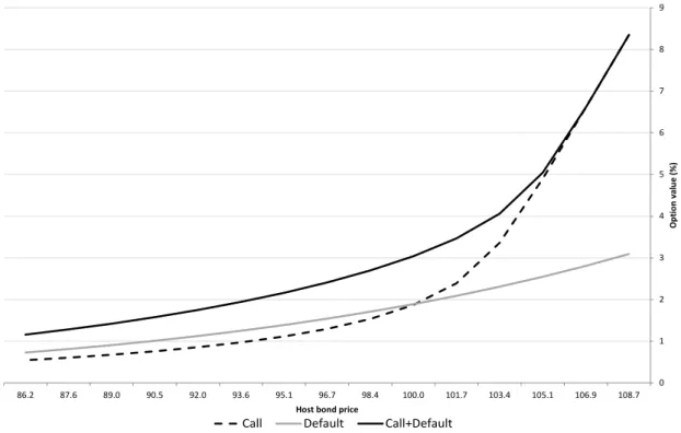
The next results describe the behaviour of a callable defaultable bond and its features, under the CIR model. As shown in Figure 2, all three bond options (callable, defaultable and callable defaultable) are concave and have a positive slope, which means that when the host bond price increases, the value of all options on that host bond increases as well. The default option is the least sensitive to the host bond price. On the other hand, the call option is the most sensitive to the host bond price, mainly on the right hand side of the curve.
21
Figure 2: The value of the options on the host bond as a function of the host bond price.
It considers three 5-year, 6.25% coupon bonds – one just callable, one just defaultable and one callable
defaultable. The instantaneous interest rate follows 𝑟𝑡= 𝜅(𝜇 − 𝑟𝑡)𝑑𝑑 + 𝜎�𝑟𝑡𝑑𝑍�𝑡; 𝜅 = 0.5, 𝜇 = 6.8%, 𝜎 = 0.10.
The firm value follows 𝑑𝑉𝑡/𝑉𝑡= (𝑟𝑡− 𝛾𝑡)𝑑𝑑 + 𝜙𝑡𝑑𝑊�𝑡; 𝛾 = 0, 𝜙 = 0.2, 𝑉0= 143. The instantaneous correlation
between the interest rate and firm value processes is −0.2.
Besides the graphic conclusion taken from Figure 2 and Figure 3, the relations between curves are supported by economic and financial theories. We notice that the call plus default option is the most valuable one and that the sum of the call option and the default option is not less than the call plus default option. The reason is that the activation of one option implies the extinguishment of the other, i.e., despite having two options, when the bond is called, the firm cannot default that bond anymore, as well as, if the firm defaults the bond, the bond won’t exist anymore and the call option won’t exist also.
p
Call Default Call+Default
0 1 2 3 4 5 6 7 8 9 108.7 106.9 105.1 103.4 101.7 100.0 98.4 96.7 95.1 93.6 92.0 90.5 89.0 87.6 86.2 O pt io n v al ue (%)
22
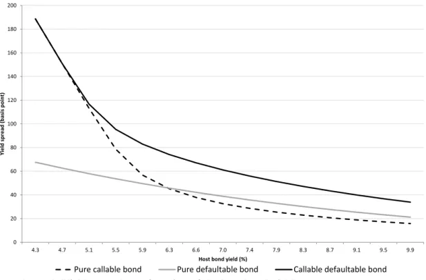
Figure 3: Yield spread as a function of the host bond yield.
It considers three 5-year, 6.25% coupon bonds – one just callable, one just defaultable and one callable
defaultable. The instantaneous interest rate follows 𝑟𝑡= 𝜅(𝜇 − 𝑟𝑡)𝑑𝑑 + 𝜎�𝑟𝑡𝑑𝑍�𝑡; 𝜅 = 0.5, 𝜇 = 6.8%, 𝜎 = 0.10.
The firm value follows 𝑑𝑉𝑡/𝑉𝑡= (𝑟𝑡− 𝛾𝑡)𝑑𝑑 + 𝜙𝑡𝑑𝑊�𝑡; 𝛾 = 0, 𝜙 = 0.2, 𝑉0= 143. The instantaneous correlation
between the interest rate and firm value processes is −0.2.
Another important results are presented in Figure 4 and Figure 5, where we can note
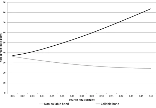
that yield spreads of non-callable and callable defaultable bonds have different behaviours for different correlation values, 𝜌.
Figure 4 shows that when the value of the firm and the cost of its debt are negatively
correlated the yield spread for a non-callable (defaultable) bond decreases smoothly as the interest rate volatility increases. The explanation stands on the smaller default risk associated to the firm, that is, the firm value will grow in the same direction of the bond value, creating an hedging effect for bond holders. As a result, the excess return over the non-callable risk-free bond becomes lower or, equivalently, the default option becomes less valuable. The behaviour of the callable defaultable bond is quite different from the non-callable one. It is justified by the relation between the call feature and the interest rate, i.e., when interest rate
Pure callable bond Pure defaultable bond Callable defaultable bond
0 20 40 60 80 100 120 140 160 180 200 4.3 4.7 5.1 5.5 5.9 6.3 6.6 7.0 7.4 7.9 8.3 8.7 9.1 9.5 9.9 Yi el d sp re ad (b as is p oi nt )
23
volatility rises, it’s plausible to observe higher values for the interest rate and, consequently, the call option becomes more expensive. This result was already achieved by Black and Scholes (1973), not exactly for a call option on a bond, but on a generic underlying asset. In addition, the yield spread of a callable defaultable bond is more sensitive to the interest rate volatility than a non-callable one.
Figure 4: Yield spread as a function of the interest rate volatility, with 𝝆 = −𝟎. 𝟓.
It considers two 10-year, 9% coupon bonds – one non-callable and one callable. The instantaneous interest rate
follows 𝑑𝑟𝑡= 𝜅(𝜇 − 𝑟𝑡)𝑑𝑑 + 𝜎�𝑟𝑡𝑑𝑍�𝑡; 𝜅 = 0.5, 𝜇 = 9%, 𝑟0= 9%. The firm value follows 𝑑𝑉𝑡/𝑉𝑡=
(𝑟𝑡− 𝛾𝑡)𝑑𝑑 + 𝜙𝑡𝑑𝑊�𝑡; 𝛾 = 0.05, 𝜙 = 0.15, 𝑉0= 123. 𝜌 is the instantaneous correlation between the interest rate
and firm value processes.
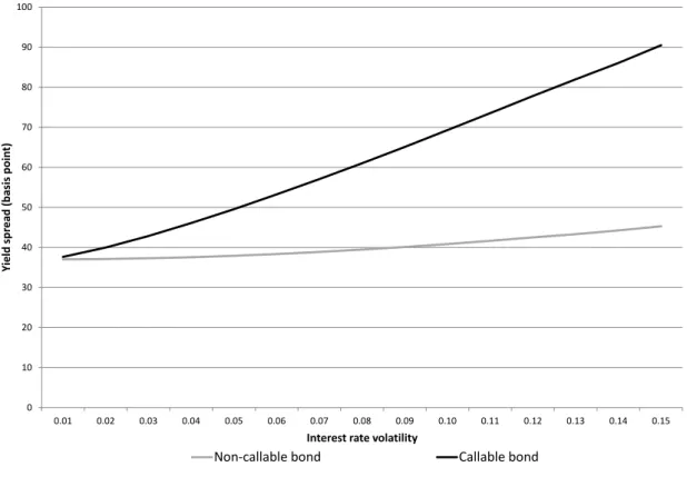
Figure 5 shows the behaviour of a callable and a non-callable defaultable bond, using
the same parameters as those used in Figure 4, but considering 𝜌 = 0. We clearly see a positive relation between yield spread and interest rate volatility for both types of bonds, even though the callable defaultable bond has a higher sensitivity to interest rate volatility than the other one. The justification is, in part, similar to the previous one. On the one hand, an increase in interest rate volatility leads to an increase of the call option value. On the other
0 10 20 30 40 50 60 70 80 90 0.01 0.02 0.03 0.04 0.05 0.06 0.07 0.08 0.09 0.10 0.11 0.12 0.13 0.14 0.15 Yi el d spr ea d ( ba si s po in t)
Interest rate volatility
Pure defaultable Callable defaultable
24
hand, the bond and firm values move on opposite ways due to the null or positive correlation and, as a result, the firm will have a higher probability to default and, thus, the higher will be the default option value as well as the yield spread.
Figure 5: The yield spread of two bonds, one non-callable and one callable, as a
function of the interest rate volatility, with 𝝆 = 𝟎. It considers two 10-year, 9% coupon bonds –
one non-callable and one callable. The instantaneous interest rate follows 𝑑𝑟𝑡= 𝜅(𝜇 − 𝑟𝑡)𝑑𝑑 + 𝜎�𝑟𝑡𝑑𝑍�𝑡; 𝜅 =
0.5, 𝜇 = 9%, 𝑟0= 9%. The firm value follows 𝑑𝑉𝑡/𝑉𝑡= (𝑟𝑡− 𝛾𝑡)𝑑𝑑 + 𝜙𝑡𝑑𝑊�𝑡; 𝛾 = 0.05, 𝜙 = 0.15, 𝑉0= 123.
𝜌 is the instantaneous correlation between the interest rate and firm value processes.
5.2. Comparison
We already know the theoretical advantage and disadvantage regarding the usage of different stochastic models on the valuation of callable defaultable bonds. However, I will present in this section an empirical comparison between three different model assumptions – the CIR model, the Vasicek model and constant interest rate – in order to say if its usage is worth or not, trading-off the differences in results and the tractability of each one.
0 10 20 30 40 50 60 70 80 90 100 0.01 0.02 0.03 0.04 0.05 0.06 0.07 0.08 0.09 0.10 0.11 0.12 0.13 0.14 0.15 Yi el d spr ea d ( ba si s po in t)
Interest rate volatility
Pure defaultable Callable defaultable
25
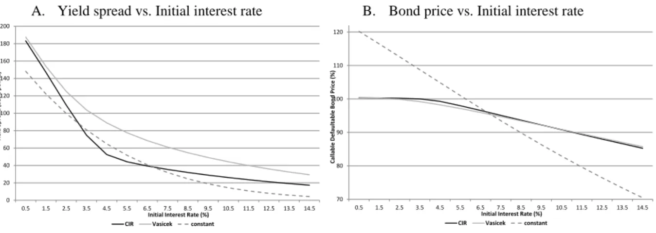
The one-factor CIR model was the preferred one to develop the results presented in the previous section, however it’s complex to work with. Figure 6 (A) and (B) present, for each interest rate model assumption, the yield spread and the price of a callable defaultable bond as a function of the initial interest rate. We unquestionably identify that the Vasicek model is the one which produces the highest values for the call plus default option. Moreover, it shows that the option value under the CIR model is the most convex ones, i.e., for lower interest rates, the value of the call plus default option is highly sensitive to the initial interest rate, whereas for higher initial interest rate, it’s only slightly sensitive. The negative convexity intrinsic to the callable bond was already referred in section 3.2 however it is perceptible on Figure 6 (B), i.e., for lower interest rates callable bonds have negative convexity (opposing to non-callable bonds).
Figure 6: Comparison of yield spreads (A) and prices (B) of a callable defaultable bond under
three interest rate model assumptions. It considers a 5-year, 6.25% coupon bond. The firm value follows 𝑑𝑉𝑡/
𝑉𝑡= (𝑟𝑡− 𝛾𝑡)𝑑𝑑 + 𝜙𝑡𝑑𝑊�𝑡; 𝛾 = 0, 𝜙 = 0.2, 𝑉0= 143. The instantaneous interest rate follows: (I) CIR: 𝑑𝑟𝑡= 𝜅(𝜇 − 𝑟𝑡)𝑑𝑑 +
𝜎�𝑟𝑡𝑑𝑍�𝑡; 𝜅 = 0.5, 𝜇 = 6.8%, 𝜎 = 2.608%; (II) Vasicek: 𝑑𝑟𝑡= 𝑎(𝑏 − 𝑟𝑡)𝑑𝑑 + 𝜎𝑑𝑍�𝑡; 𝑎 = 0.5, 𝑏 = 6.8%; 𝜎 = 2.608%. The
instantaneous correlation between the interest rate and firm value processes is −0.2.
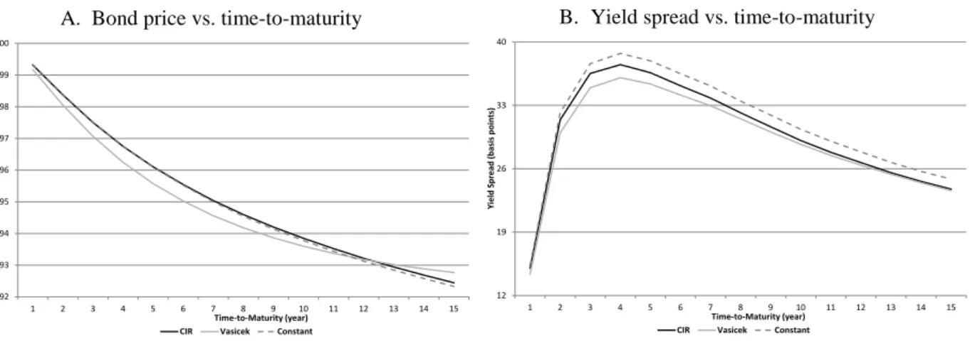
Another pertinent question is related to time-to-maturity, i.e., what happens to the yield spreads and bond values when we value a callable defaultable bond with higher time-to-maturity. Figure 7 (A) and (B) answer this question. For all 3 assumptions, it is notable that the higher yield spread is situated around 4 years. Furthermore, for short times-to-maturity the 3 assumptions are quite similar whereas for long times-to-maturity just the CIR and the
0 20 40 60 80 100 120 140 160 180 200 0.5 1.5 2.5 3.5 4.5 5.5 6.5 7.5 8.5 9.5 10.5 11.5 12.5 13.5 14.5 Yie ld S pr ead (b as is p oin ts )
Initial Interest Rate (%) CIR Vasicek constant
70 80 90 100 110 120 0.5 1.5 2.5 3.5 4.5 5.5 6.5 7.5 8.5 9.5 10.5 11.5 12.5 13.5 14.5 Callab le De fau ltab le B on d P ric e ( % )
Initial Interest Rate (%) CIR Vasicek constant
B. Bond price vs. Initial interest rate A. Yield spread vs. Initial interest rate
26
Vasicek model assumptions give similar results. While the callable defaultable bond price under the CIR model is more convex as function of the initial interest rate, for variations on time-to-maturity the callable defaultable bond price under the Vasicek model presents more convexity instead.
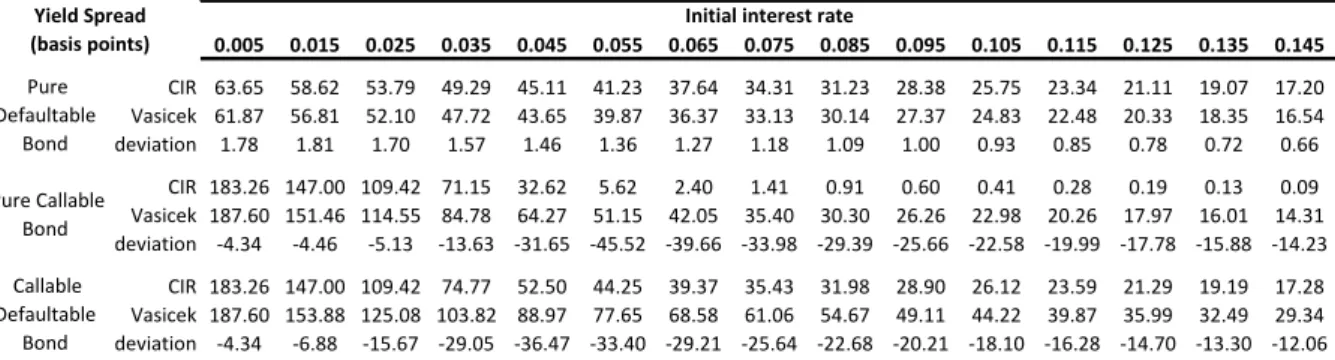
Table 2 and Table 3 show how similar are the results under the CIR and the Vasicek
models, for option values and yield spreads. The default option on the host bond is the most similar between those two assumptions, even though the highest differences are registered for lower interest rates. The most significant differences are registered in call options and are localized near to the coupon rate value. Of course, the interest rate region near to the bond coupon rate is the critical one as the call option has higher probability to be activated and any marginal divergence movement causes differences in the valuation of the option.
We verify the same behaviour for yield spreads, however with a different magnitude. The differences in yield spreads of a defaultable bond are, in fact, insignificant whereas in yield spreads of a callable bond is already relevant, more intensively for initial interest rates near to the bond coupon rate as it happens for call options.
12 19 26 33 40 1 2 3 4 5 6 7 8 9 10 11 12 13 14 15 Yie ld S pr ead (b as is p oin ts ) Time-to-Maturity (year) CIR Vasicek Constant
92 93 94 95 96 97 98 99 100 1 2 3 4 5 6 7 8 9 10 11 12 13 14 15 Callab le De fau ltab le B on d P ric e ( % ) Time-to-Maturity (year) CIR Vasicek Constant
B. Yield spread vs. time-to-maturity A. Bond price vs. time-to-maturity
Figure 7: Comparison of prices (A) and yield spreads (B) of a callable defaultable bond under three
interest rate model assumptions. It considers a 6.25% coupon bond. The firm value follows 𝑑𝑉𝑡/𝑉𝑡= (𝑟𝑡− 𝛾𝑡)𝑑𝑑 +
𝜙𝑡𝑑𝑊�𝑡; 𝛾 = 0, 𝜙 = 0.2, 𝑉0= 143. The instantaneous interest rate follows: (I) CIR: 𝑑𝑟𝑡= 𝜅(𝜇 − 𝑟𝑡)𝑑𝑑 + 𝜎�𝑟𝑡𝑑𝑍�𝑡; 𝜅 = 0.5, 𝜇 =
6.8%, 𝑟0= 6.8%, 𝜎 = 2.608%; (II) Vasicek: 𝑑𝑟𝑡= 𝑎(𝑏 − 𝑟𝑡)𝑑𝑑 + 𝜎𝑑𝑍�𝑡; 𝑎 = 0.5, 𝑏 = 6.8%, 𝑟0= 6.8%, 𝜎 = 2.608%; (III)
27
Table 2: Comparison of prices of a default, a call and a call+default options on the host bond
under two stochastic interest rate models, over different levels of the initial interest rate. It
considers a 5-year, 6.25% coupon bond. The firm value follows 𝑑𝑉𝑡/𝑉𝑡= (𝑟𝑡− 𝛾𝑡)𝑑𝑑 + 𝜙𝑡𝑑𝑊�𝑡; 𝛾 = 0, 𝜙 = 0.2, 𝑉0= 143.
The instantaneous interest rate follows: (I) CIR: 𝑑𝑟𝑡= 𝜅(𝜇 − 𝑟𝑡)𝑑𝑑 + 𝜎�𝑟𝑡𝑑𝑍�𝑡; 𝜅 = 0.5, 𝜇 = 6.8%, 𝜎 = 2.608%; (II)
Vasicek: 𝑑𝑟𝑡= 𝑎(𝑏 − 𝑟𝑡)𝑑𝑑 + 𝜎𝑑𝑍�𝑡; 𝑎 = 0.5, 𝑏 = 6.8%, 𝜎 = 2.608%; The instantaneous correlation between the interest
rate and firm value processes is −0.2.
Table 3: Comparison of yield spreads of a defaultable, a callable and a callable defaultable bond
under two stochastic interest rate models, over different levels of the initial interest rate. It
considers a 5-year, 6.25% coupon bond. The firm value follows 𝑑𝑉𝑡/𝑉𝑡= (𝑟𝑡− 𝛾𝑡)𝑑𝑑 + 𝜙𝑡𝑑𝑊�𝑡; 𝛾 = 0, 𝜙 = 0.2, 𝑉0= 143.
The instantaneous interest rate follows: (I) CIR: 𝑑𝑟𝑡= 𝜅(𝜇 − 𝑟𝑡)𝑑𝑑 + 𝜎�𝑟𝑡𝑑𝑍�𝑡; 𝜅 = 0.5, 𝜇 = 6.8%, 𝜎 = 2.608%; (II)
Vasicek: 𝑑𝑟𝑡= 𝑎(𝑏 − 𝑟𝑡)𝑑𝑑 + 𝜎𝑑𝑍�𝑡; 𝑎 = 0.5, 𝑏 = 6.8%, 𝜎 = 2.608%; The instantaneous correlation between the interest
rate and firm value processes is −0.2.
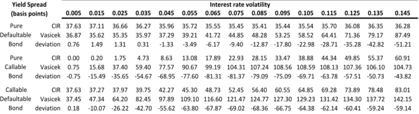
An additional parameter that is relevant when we are testing different interest rate models is the interest rate volatility and how option prices and yield spreads respond to it. As
Table 4 shows, the call option as well as the call+default option under the Vasicek model are
more sensitive for lower values of the interest rate volatility than under the CIR model, and after certain point the option value decreases. The CIR model produces more consistent values as it is rational to increase the value of an option when the volatility of its underlying instrument is increased as well. Regarding the default option valuation, the CIR model, once
0.005 0.015 0.025 0.035 0.045 0.055 0.065 0.075 0.085 0.095 0.105 0.115 0.125 0.135 0.145 CIR 2.91 2.62 2.36 2.12 1.90 1.70 1.52 1.36 1.21 1.08 0.96 0.85 0.75 0.67 0.59 Vasicek 2.83 2.55 2.30 2.06 1.85 1.66 1.48 1.32 1.18 1.05 0.93 0.83 0.73 0.65 0.57 deviation 0.07 0.07 0.06 0.06 0.05 0.04 0.04 0.04 0.03 0.03 0.02 0.02 0.02 0.02 0.01 CIR 8.10 6.43 4.73 3.04 1.38 0.23 0.10 0.06 0.04 0.02 0.02 0.01 0.01 0.00 0.00 Vasicek 8.30 6.64 4.97 3.63 2.71 2.12 1.71 1.41 1.19 1.01 0.86 0.75 0.65 0.57 0.50 deviation -0.20 -0.21 -0.24 -0.59 -1.33 -1.89 -1.61 -1.36 -1.15 -0.98 -0.85 -0.74 -0.64 -0.56 -0.49 CIR 8.10 6.43 4.73 3.19 2.21 1.82 1.59 1.40 1.24 1.10 0.97 0.86 0.76 0.67 0.59 Vasicek 8.30 6.74 5.41 4.42 3.73 3.19 2.77 2.42 2.13 1.87 1.65 1.46 1.29 1.14 1.01 deviation -0.20 -0.31 -0.68 -1.23 -1.52 -1.37 -1.18 -1.02 -0.89 -0.78 -0.68 -0.60 -0.53 -0.47 -0.42
Initial interest rate
Default Call Call+Default Option Value (%) 0.005 0.015 0.025 0.035 0.045 0.055 0.065 0.075 0.085 0.095 0.105 0.115 0.125 0.135 0.145 CIR 63.65 58.62 53.79 49.29 45.11 41.23 37.64 34.31 31.23 28.38 25.75 23.34 21.11 19.07 17.20 Vasicek 61.87 56.81 52.10 47.72 43.65 39.87 36.37 33.13 30.14 27.37 24.83 22.48 20.33 18.35 16.54 deviation 1.78 1.81 1.70 1.57 1.46 1.36 1.27 1.18 1.09 1.00 0.93 0.85 0.78 0.72 0.66 CIR 183.26 147.00 109.42 71.15 32.62 5.62 2.40 1.41 0.91 0.60 0.41 0.28 0.19 0.13 0.09 Vasicek 187.60 151.46 114.55 84.78 64.27 51.15 42.05 35.40 30.30 26.26 22.98 20.26 17.97 16.01 14.31 deviation -4.34 -4.46 -5.13 -13.63 -31.65 -45.52 -39.66 -33.98 -29.39 -25.66 -22.58 -19.99 -17.78 -15.88 -14.23 CIR 183.26 147.00 109.42 74.77 52.50 44.25 39.37 35.43 31.98 28.90 26.12 23.59 21.29 19.19 17.28 Vasicek 187.60 153.88 125.08 103.82 88.97 77.65 68.58 61.06 54.67 49.11 44.22 39.87 35.99 32.49 29.34 deviation -4.34 -6.88 -15.67 -29.05 -36.47 -33.40 -29.21 -25.64 -22.68 -20.21 -18.10 -16.28 -14.70 -13.30 -12.06 Pure Callable Bond Callable Defaultable Bond
Initial interest rate Pure
Defaultable Bond
Yield Spread (basis points)
28
again, seems to give more consistent results as it shows that the value of the default option is not sensitive to interest rate volatility. Table 5 presents the sensitivity of yield spread to the interest rate volatility. Similarly to Table 4, the yield spread of the callable bond under the Vasicek model presents a huge increase as a response to the increase of the interest rate volatility up to the level of 7.5%, from which it starts to decrease. This behaviour has no fundaments since interest rate volatility is assumed constant and there is no stochastic model for it.
Table 4: Comparison of prices of a default, a call and a call+default option on the host bond
under two stochastic interest rate models, over different levels of interest rate volatility. It considers
a 5-year, 6.25% coupon bond. The firm value follows 𝑑𝑉𝑡/𝑉𝑡= (𝑟𝑡− 𝛾𝑡)𝑑𝑑 + 𝜙𝑡𝑑𝑊�𝑡; 𝛾 = 0, 𝜙 = 0.2, 𝑉0= 143. The
instantaneous interest rate follows: (I) CIR: 𝑑𝑟𝑡= 𝜅(𝜇 − 𝑟𝑡)𝑑𝑑 + 𝜎�𝑟𝑡𝑑𝑍�𝑡; 𝜅 = 0.5, 𝜇 = 6.8%, 𝑟0= 6.8%; (II) Vasicek:
𝑑𝑟𝑡= 𝑎(𝑏 − 𝑟𝑡)𝑑𝑑 + 𝜎𝑑𝑍�𝑡; 𝑎 = 0.5, 𝑏 = 6.8%, 𝑟0= 6.8%; The instantaneous correlation between the interest rate and firm
value processes is −0.2.
Table 5: Comparison of yield spreads of a defaultable, a callable and a callable defaultable bond
under two stochastic interest rate models, over different levels of interest rate volatility. It considers
a 5-year, 6.25% coupon bond. The firm value follows 𝑑𝑉𝑡/𝑉𝑡= (𝑟𝑡− 𝛾𝑡)𝑑𝑑 + 𝜙𝑡𝑑𝑊�𝑡; 𝛾 = 0, 𝜙 = 0.2, 𝑉0= 143. The
instantaneous interest rate follows: (I) CIR: 𝑑𝑟𝑡= 𝜅(𝜇 − 𝑟𝑡)𝑑𝑑 + 𝜎�𝑟𝑡𝑑𝑍�𝑡; 𝜅 = 0.5, 𝜇 = 6.8%, 𝑟0= 6.8%; (II) Vasicek:
𝑑𝑟𝑡= 𝑎(𝑏 − 𝑟𝑡)𝑑𝑑 + 𝜎𝑑𝑍�𝑡; 𝑎 = 0.5, 𝑏 = 6.8%, 𝑟0= 6.8%; The instantaneous correlation between the interest rate and firm
value processes is −0.2. 0.005 0.015 0.025 0.035 0.045 0.055 0.065 0.075 0.085 0.095 0.105 0.115 0.125 0.135 0.145 CIR 1.51 1.49 1.47 1.46 1.45 1.44 1.43 1.43 1.43 1.43 1.43 1.44 1.46 1.47 1.47 Vasicek 1.49 1.44 1.43 1.46 1.51 1.58 1.67 1.79 1.91 2.08 2.26 2.46 2.69 2.94 3.21 deviation 0.02 0.05 0.04 0.00 -0.07 -0.15 -0.24 -0.36 -0.48 -0.65 -0.83 -1.02 -1.23 -1.48 -1.74 CIR 0.00 0.01 0.07 0.19 0.35 0.53 0.72 0.93 1.14 1.35 1.57 1.78 2.00 2.23 2.45 Vasicek 0.03 0.64 1.51 2.39 3.11 3.61 3.92 4.09 4.17 4.18 4.14 4.08 4.01 3.92 3.83 deviation -0.03 -0.63 -1.44 -2.20 -2.76 -3.08 -3.20 -3.16 -3.03 -2.83 -2.57 -2.30 -2.00 -1.69 -1.38 CIR 1.51 1.50 1.52 1.60 1.70 1.82 1.95 2.10 2.26 2.42 2.59 2.77 2.95 3.13 3.31 Vasicek 1.51 1.91 2.58 3.30 3.90 4.32 4.59 4.74 4.83 4.88 4.90 4.93 4.98 5.04 5.14 deviation 0.00 -0.41 -1.05 -1.71 -2.21 -2.51 -2.64 -2.64 -2.57 -2.46 -2.31 -2.16 -2.03 -1.91 -1.83
Interest rate volatility
Default Call Call+Default Option Value (%) 0.005 0.015 0.025 0.035 0.045 0.055 0.065 0.075 0.085 0.095 0.105 0.115 0.125 0.135 0.145 CIR 37.63 37.11 36.66 36.27 35.96 35.72 35.55 35.45 35.41 35.44 35.54 35.70 36.08 36.35 36.28 Vasicek 36.87 35.62 35.35 35.97 37.29 39.21 41.72 44.85 48.28 53.25 58.52 64.41 71.36 79.17 87.49 deviation 0.76 1.49 1.31 0.31 -1.33 -3.49 -6.17 -9.40 -12.87 -17.80 -22.98 -28.71 -35.28 -42.82 -51.21 CIR 0.00 0.20 1.75 4.73 8.63 13.08 17.89 22.93 28.15 33.47 38.88 44.34 49.85 55.37 60.91 Vasicek 0.75 15.68 37.40 59.40 77.57 90.67 99.19 104.31 107.24 108.56 108.59 108.13 107.36 106.10 104.73 deviation -0.75 -15.49 -35.65 -54.67 -68.95 -77.60 -81.31 -81.37 -79.09 -75.09 -69.71 -63.78 -57.51 -50.73 -43.82 CIR 37.63 37.27 37.97 39.75 42.27 45.30 48.73 52.45 56.40 60.55 64.85 69.28 73.89 78.48 83.01 Vasicek 37.45 47.34 64.20 82.45 97.89 109.10 116.60 121.47 124.77 127.30 129.23 131.42 134.30 137.72 142.15 deviation 0.18 -10.07 -26.22 -42.70 -55.62 -63.80 -67.87 -69.02 -68.36 -66.75 -64.38 -62.14 -60.41 -59.24 -59.14 Pure Defaultable Bond Pure Callable Bond Callable Defaultable Bond
Interest rate volatility Yield Spread
29
Chapter 6
Conclusion
Attending to the valuation and analysis of callable defaultable bonds, as well as of pure callable bonds and pure defaultable bonds presented in the previous chapters, we can achieve several conclusions.
Under the CIR model assumption for the interest rate behaviour, our numerical results show that the value of all three types of options on the host bond are positively related with the value of its host bond price and the call+default option is the most valuable one as the theory says, even though the call option is also the most convex one. Similar results are verified on yield spreads of each bond for different levels of host bond yield. Unsurprisingly, the yield spread of the callable defaultable bond is the highest one since it is riskier, due to the default risk and the earlier redemption risk.
An additional sensitivity analysis presented in this thesis is related to the behaviour of the yield spread of callable and non-callable (defaultable) bonds with respect to the variation on the interest rate volatility, under different values for correlation between 𝑟 and 𝑉. The yield spread of a non-callable bond is positively related to interest rate volatility when 𝜌 is positive, and negatively related when 𝜌 is negative. However the yield spread of a callable bond is always positive. Unlike Acharya and Carpenter (2002) affirm, when 𝜌 is negative, the yield spread of a callable defaultable bond is positively related to interest rate volatility and it intensifies when 𝜌 is higher. The theoretical arguments are the following: (i) the increase on the interest rate volatility leads to an increase of the call option as its underlying instrument becomes more volatile; (ii) the correlation values just affect the default option; (iii) the variations on interest rates are partially reflected in the firm value (depending on the correlation value), and consequently in the value of a callable bond; (iv) even if changes on interest rate cause changes in opposite way on the firm value, the firm value is directly and positively dependent of the interest rate values, which means that there is another factor that shrinks the effect caused by the negative correlation.
30
Due to the doubts about the advantage of using the CIR model, the Vasicek model or even constant interest rate, the previous section offers arguments that support the CIR model assumption. In fact, the valuation of callable defaultable bonds under the assumption of a constant interest rate, as Merton (1974) suggested, is only acceptable when the bond has a short maturity.
The price of a callable defaultable bond is quite similar between the CIR model and Vasicek model over different levels of initial interest rate, except for those ones near to the coupon rate where it points small deviations. Moreover, the yield spread of the callable defaultable bond over different levels of initial interest rate is more convex under the CIR model than under the Vasicek model. The main divergence between both models starts on the interest rate volatility analysis. By analysing the call option value or the yield spread of the pure callable bond under the Vasicek model, we verify an unreasonable behaviour over different levels of interest rate volatility, i.e., the call option, for instance, exhibits a huge increase on its value as the interest rate volatility increases until certain point, after that it becomes stable whereas the same option, under the CIR model, presents a smooth line with positive slope.
The callable defaultable bond pricing model, under two stochastic processes – one for firm value and one for the interest rate – seemed to improve its goodness of fit, as Acharya and Carpenter (2002) noted. However the implementation issues are enormous, and all related to computational capacity. In this case, Matlab wastes a lot of memory to build a 3-dimensional matrix since most of the cells are not used.
31
Bibliography
Acharya, Viral V., and Jennifer N. Carpenter. “Corporate Bond Valuation and Hedging with Stochastic Interest Rates and Endogenous Bankrupcy.” The Review of Financial
Studies 15 (Winter 2002): 1355-1383.
Black, Fischer, and Myron Scholes. “The princing of Options and Corporate Liabilities.” The
Journal of Political Economy, 1973: 637-654.
Brealey, Richard A., and Stewart C. Myers. Principles of Corporate Finance. 7ed. Mcgraw-Hill Companies, 2003.
Brennan, M. J., and E. S. Schwartz. “Convertible Bonds: Valuation and Optimal Strategies for Call and Conversion.” Jornal of Finance, 1977: 1699-1715.
Cox, John C., Jonathan E. Ingersoll, and Stephen A Ross. “An Intertemporal General Equilibrium Model of Asset Prices.” Econometrica 53 (March 1985): 363-384.
Duffie, Darell, and Kenneth J. Singleton. “Modeling Term Structures of Defaultable Bonds.”
Review of Financial Studies, 1999: 45.
Hull, John C., Izzy Nelken, and Alan D. White. “Merton’s model, credit risk and volatility skews.” Journal of Credit Risk, 2004.
Jarrow, Robert, Li Haitao, Sheen Liu, and Chunchi Wu. “Reduced-Form Valuation of Callable Corporate Bonds: Theoryand Evidence.” 2006.
Jones, E. Philip, Scott P. Mason, and Eric Rosenfield. “Contingent Claims Analysis of Corporate Capital Structures: An Empirical Investigation.” The Journal of Finance, 1984: 611-625.
32
Longstaff, Francis A., and Eduardo S. Schwartz. “Interest Rate Volatility and the Term Structure: A Two-Factor General Equilibrium Model.” The Journal of Finance, 1992.
Merton, Robert C. “On the Princing of Corporate Debt: The Risk Structure of Interest Rate.”
Jornal of Finance, 1974: 449-470.
Vasicek, Oldrich. “An Equilibrium Characterization of the Term Structure.” Journal of
33
Appendix A
Matlab codes
A.1. Inputs
step – number of time-steps of the tree; T – time-to-maturity;
F – face value of the bond; C – coupon rate;
strike – the value which the issuer has the right to call the bond; v0 – initial firm value;
r0 – initial interest rate;
miu – long-term value for the interest rate;
kapa – speed of adjustment to the long-term value; sigma – interest rate volatility;
gama – continuous dividend yield; phi – volatility of the firm’s return;
roh – correlation between the interest rate and firm value processes. slack – auxiliary variable to fit the matrix dimension
A.2. Import data function
function read_function(fileToRead,sheet) [numbers, strings] = xlsread(fileToRead,sheet); if ~isempty(numbers)newData1.data = numbers; end
if ~isempty(strings) && ~isempty(numbers) [strRows, strCols] = size(strings); [numRows, ~] = size(numbers);
34
% Break the data up into a new structure with one field per row. if strCols == 1 && strRows == numRows
newData1.rowheaders = strings(:,end); end
end
% Create new variables in the base workspace from those fields. for i = 1:size(newData1.rowheaders, 1)
assignin('base', genvarname(newData1.rowheaders{i}), newData1.data(i,:)); end
A.3. Callable defaultable bond value et al. under CIR model
This code retrieves the value of the host bond, the pure callable bond, the pure defaultable bond, the callable defaultable bond as well as the value of the call option, the default option and the call+default option on the host bond.
clear all; %Import Data
read_function('data_cir.xls','Input') tic
mid=step+slack; %define the center of the matrix dt=T/(step-1); %time increment
dc=C*T/(step-1); %coupon increment
%Inicialization the matrices with zeros X=zeros(mid*2-1,step);
Y=zeros(mid*2-1,step); V=zeros(mid*2-1,step);
35 K1=zeros(mid*2-1,mid*2-1,step); K2=zeros(mid*2-1,mid*2-1,step); P=zeros(mid*2-1,mid*2-1,step); Q=zeros(mid*2-1,mid*2-1,step); %Calculation at time n=1 V(mid,1)=v0; R(mid,mid,1)=r0; X(mid,1)=log(v0)/phi; Y(mid,1)=(2/sigma*sqrt(r0)-roh*X(mid,1))/sqrt(1-roh^2); miup=(R(mid,mid,1)-gama-phi^2/2)/phi; miud=(-roh*miup+(kapa*miu-sigma^2/4-kapa*R(mid,mid,1))/(sigma*sqrt(R(mid,mid,1))))/sqrt(1-roh^2); k1up=(miup*sqrt(dt)+1)/2; k1down=(miup*sqrt(dt)-1)/2; if(ceil(k1down)>0) K1(mid,mid,1)=ceil(k1down); else if(floor(k1up)>0) K1(mid,mid,1)=0; end K1(mid,mid,1)=floor(k1up); end k2up=(miud*sqrt(dt)+1)/2; k2down=(miud*sqrt(dt)-1)/2; if(ceil(k2down)>0) K2(mid,mid,1)=ceil(k2down); else if(floor(k2up)>0) K2(mid,mid,1)=0; end
36
K2(mid,mid,1)=floor(k2up); end
P(mid,mid,1)=(1+miup*sqrt(dt))/2-K1(mid,mid,1); Q(mid,mid,1)=(1+miud*sqrt(dt))/2-K2(mid,mid,1); clear miup miud k1up k1down k2up k2down;
%Tree for V and R for n=2:1:step for i=-(mid-1):1:(mid-1) if (V(mid+i,n-1)>0) for j=-(mid-1):1:(mid-1) if(R(mid+i,mid+j,n-1)>0) % up-up k1=K1(mid+i,mid+j,n-1); k2=K2(mid+i,mid+j,n-1); X(mid+i+(2*k1+1),n)=X(mid+i,n-1)+(2*k1+1)*sqrt(dt); Y(mid+j+(2*k2+1),n)=Y(mid+j,n-1)+(2*k2+1)*sqrt(dt); V(mid+i+(2*k1+1),n)=exp(phi*X(mid+i+(2*k1+1),n)); R(mid+i+(2*k1+1),mid+j+(2*k2+1),n)=((sigma/2)*(sqrt(1-roh^2)* Y(mid+j+(2*k2+1),n)+roh*X(mid+i+(2*k1+1),n)))^2; miup=(R(mid+i+(2*k1+1),mid+j+(2*k2+1),n)-gama-phi^2/2)/phi; miud=(-roh*miup+(kapa*miu-sigma^2/4-kapa* R(mid+i+(2*k1+1),mid+j+(2*k2+1),n))/ (sigma*sqrt(R(mid+i+(2*k1+1),mid+j+(2*k2+1),n))))/sqrt(1-roh^2); k1up=(miup*sqrt(dt)+1)/2; k1down=(miup*sqrt(dt)-1)/2; if(ceil(k1down)>0) K1(mid+i+(2*k1+1),mid+j+(2*k2+1),n)=ceil(k1down); else if(floor(k1up)>0) K1(mid+i+(2*k1+1),mid+j+(2*k2+1),n)=0;
37 end K1(mid+i+(2*k1+1),mid+j+(2*k2+1),n)=floor(k1up); end k2up=(miud*sqrt(dt)+1)/2; k2down=(miud*sqrt(dt)-1)/2; if(ceil(k2down)>0) K2(mid+i+(2*k1+1),mid+j+(2*k2+1),n)=ceil(k2down); else if(floor(k2up)>0) K2(mid+i+(2*k1+1),mid+j+(2*k2+1),n)=0; end K2(mid+i+(2*k1+1),mid+j+(2*k2+1),n)=floor(k2up); end P(mid+i+(2*k1+1),mid+j+(2*k2+1),n)=(1+miup*sqrt(dt))/2- K1(mid+i+(2*k1+1),mid+j+(2*k2+1),n); Q(mid+i+(2*k1+1),mid+j+(2*k2+1),n)=(1+miud*sqrt(dt))/2- K2(mid+i+(2*k1+1),mid+j+(2*k2+1),n);
clear miup miud k1up k1down k2up k2down; %up-down X(mid+i+(2*k1+1),n)=X(mid+i,n-1)+(2*k1+1)*sqrt(dt); Y(mid+j+(2*k2-1),n)=Y(mid+j,n-1)+(2*k2-1)*sqrt(dt); V(mid+i+(2*k1+1),n)=exp(phi*X(mid+i+(2*k1+1),n)); R(mid+i+(2*k1+1),mid+j+(2*k2-1),n)=((sigma/2)*(sqrt(1-roh^2)* Y(mid+j+(2*k2-1),n)+roh*X(mid+i+(2*k1+1),n)))^2; miup=(R(mid+i+(2*k1+1),mid+j+(2*k2-1),n)-gama-phi^2/2)/phi; miud=(-roh*miup+(kapa*miu-sigma^2/4-kapa* R(mid+i+(2*k1+1),mid+j+(2*k2-1),n))/ (sigma*sqrt(R(mid+i+(2*k1+1),mid+j+(2*k2-1),n))))/sqrt(1-roh^2); k1up=(miup*sqrt(dt)+1)/2; k1down=(miup*sqrt(dt)-1)/2;
38 if(ceil(k1down)>0) K1(mid+i+(2*k1+1),mid+j+(2*k2-1),n)=ceil(k1down); else if(floor(k1up)>0) K1(mid+i+(2*k1+1),mid+j+(2*k2-1),n)=0; end K1(mid+i+(2*k1+1),mid+j+(2*k2-1),n)=floor(k1up); end k2up=(miud*sqrt(dt)+1)/2; k2down=(miud*sqrt(dt)-1)/2; if(ceil(k2down)>0) K2(mid+i+(2*k1+1),mid+j+(2*k2-1),n)=ceil(k2down); else if(floor(k2up)>0) K2(mid+i+(2*k1+1),mid+j+(2*k2-1),n)=0; end K2(mid+i+(2*k1+1),mid+j+(2*k2-1),n)=floor(k2up); end P(mid+i+(2*k1+1),mid+j+(2*k2-1),n)=(1+miup*sqrt(dt))/2- K1(mid+i+(2*k1+1),mid+j+(2*k2-1),n); Q(mid+i+(2*k1+1),mid+j+(2*k2-1),n)=(1+miud*sqrt(dt))/2- K2(mid+i+(2*k1+1),mid+j+(2*k2-1),n);
clear miup miud k1up k1down k2up k2down; %down-up X(mid+i+(2*k1-1),n)=X(mid+i,n-1)+(2*k1-1)*sqrt(dt); Y(mid+j+(2*k2+1),n)=Y(mid+j,n-1)+(2*k2+1)*sqrt(dt); V(mid+i+(2*k1-1),n)=exp(phi*X(mid+i+(2*k1-1),n)); R(mid+i+(2*k1-1),mid+j+(2*k2+1),n)=((sigma/2)*(sqrt(1-roh^2)* Y(mid+j+(2*k2+1),n)+roh*X(mid+i+(2*k1-1),n)))^2; miup=(R(mid+i+(2*k1-1),mid+j+(2*k2+1),n)-gama-phi^2/2)/phi;