doi:10.5194/amt-9-2315-2016
© Author(s) 2016. CC Attribution 3.0 License.
Consistency and quality assessment of the Metop-A/IASI and
Metop-B/IASI operational trace gas products (O
3
, CO, N
2
O,
CH
4
, and CO
2
) in the subtropical North Atlantic
Omaira Elena García1, Eliezer Sepúlveda1, Matthias Schneider2, Frank Hase2, Thomas August3, Thomas Blumenstock2, Sven Kühl1, Rosemary Munro3, Ángel Jesús Gómez-Peláez1, Tim Hultberg3, Alberto Redondas1, Sabine Barthlott2, Andreas Wiegele2, Yenny González1, and Esther Sanromá1 1Izaña Atmospheric Research Centre (IARC), Agencia Estatal de Meteorología (AEMET),
Santa Cruz de Tenerife, Spain
2Institute of Meteorology and Climate Research (IMK-ASF), Karlsruhe Institute of Technology (KIT), Karlsruhe, Germany
3European Organisation for the Exploitation of Meteorological Satellites (EUMETSAT), Darmstadt, Germany
Correspondence to:Omaira Elena García (ogarciar@aemet.es)
Received: 10 November 2015 – Published in Atmos. Meas. Tech. Discuss.: 21 December 2015 Revised: 10 May 2016 – Accepted: 12 May 2016 – Published: 25 May 2016
Abstract.This paper presents the tools and methodology for performing a routine comprehensive monitoring of consis-tency and quality of IASI (Infrared Atmospheric Sounding Interferometer) trace gas Level 2 (L2) products (O3, CO, N2O, CH4, and CO2) generated at EUMETSAT (European Organisation for the Exploitation of Meteorological Satel-lites) using ground-based observations at the Izaña Atmo-spheric Observatory (IZO, Tenerife). As a demonstration the period 2010–2014 was analysed, covering the version 5 of the IASI L2 processor. Firstly, we assess the consistency be-tween the total column (TC) observations from the IASI sen-sors on board the EUMETSAT Metop-A and Metop-B me-teorological satellites (IASI-A and IASI-B respectively) in the subtropical North Atlantic region during the first 2 years of IASI-B operations (2012–2014). By analysing different timescales, we probe the daily and annual consistency of the variability observed by IASI-A and IASI-B and thereby as-sess the suitability of B for continuation of the IASI-A time series. The continuous intercomparison of both IIASI-ASI sensors also offers important diagnostics for identifying in-consistencies between the data records and for documenting their temporal stability. Once the consistency of IASI sen-sors is documented we estimate the overall accuracy of all the IASI trace gas TC products by comparing to coincident
ground-based Fourier transform infrared spectrometer (FTS) measurements performed at IZO from 2010 to 2014. The IASI L2 products reproduce the ground-based FTS obser-vations well at the longest temporal scales, i.e. annual cy-cles and long-term trends for all the trace gases considered (Pearson correlation coefficient,R, larger than 0.95 and 0.75
for long-term trends and annual cycles respectively) with the exception of CO2. For CO2 acceptable agreement is only achieved for long-term trends (R∼0.70). The differences
observed between IASI and FTS observations can be in part attributed to the different vertical sensitivities of the two re-mote sensing instruments and also to the degree of maturity of the IASI products: O3and CO are pre-operational, while N2O, CH4, and CO2are, for the period covered by this study, aspirational products only and are not considered mature. Re-garding shorter timescales (single or daily measurements), only the O3product seems to show good sensitivity to actual atmospheric variations (R∼0.80), while the CO product is
only moderately sensitive (R∼0.50). For the remainder of
1 Introduction
Continuous, consistent, and high-quality long-term monitor-ing of the composition of the atmosphere is fundamental for addressing the challenges of climate research. In this con-text space-based remote sensing observations are of particu-lar importance, since they are unique in providing a global coverage. Among the current space-based remote sensing instruments, IASI (Infrared Atmospheric Sounding Interfer-ometer, Blumstein et al., 2004) has special relevance since it combines high quality (very good signal-to-noise ratio and high spectral resolution), good horizontal resolution (12 km at nadir), global coverage, and long-term data availability. Its mission is guaranteed until 2022 through the meteorological satellites Metop, the space component of the EUMETSAT (European Organisation for the Exploitation of Meteorolog-ical Satellites) Polar System (EPS) programme: the first sen-sor (IASI-A) was launched in October 2006 on board Metop-A, the second (IASI-B) was launched in September 2012 on board Metop-B, and the third (IASI-C) is expected to be launched in October 2018 aboard Metop-C. A successor to IASI, IASI-NG (Crevoisier et al., 2014), with improved spec-tral resolution and radiometric performance is under develop-ment as part of the EPS-SG (Second Generation) programme and will continue the mission after Metop-C and extend the data record by 2 decades. All these features make the IASI missions very promising for monitoring atmospheric com-position in the long term as a key instrument for the EU-METSAT Earth observation programme (e.g. Clerbaux et al., 2009; Crevoisier et al., 2009a, b; Herbin et al., 2009; Schnei-der and Hase, 2011; August et al., 2012; Kerzenmacher et al., 2012). However, for correct scientific use of these long-term observational records, an assessment of the consistency of the atmospheric observations from the IASI sensors currently in orbit, as well as a documentation of their quality is re-quired. To date there has been no comprehensive consistency and validation study for all the trace gas products dissemi-nated by EUMETSAT as IASI Level 2 (L2) products. Such activities have been mostly performed in the context of short campaigns or have been focused on specific atmospheric pa-rameters (e.g. Keim et al., 2009; Viatte et al., 2011; Schnei-der and Hase, 2011; García et al., 2013). By such campaigns alone it is not possible to extensively evaluate the quality of the different IASI atmospheric products as well as the poten-tial of IASI for long-term climate studies. In order to address these two critical tasks, high-quality ground-based reference data sets are needed.
While there are several techniques for measuring total col-umn (TC) amounts of atmospheric trace gases such as water vapour or ozone that can be used as a validation reference (e.g. radiosondes, UV–VIS spectrometers), there is currently only one technique that routinely estimates all the atmo-spheric trace gases retrieved operationally from IASI mea-surements (ozone, O3, carbon monoxide, CO, nitrous oxide, N2O, methane, CH4, and carbon dioxide, CO2): the
ground-based Fourier transform spectrometers (FTSs). FTS instru-ments record very high-resolution infrared solar absorption spectra and use a similar measurement approach as IASI. By evaluating these solar spectra, the FTS systems can pro-vide TC amounts and volume mixing ratio (VMR) profiles of many different atmospheric trace gases with high precision. Within the NDACC (Network for Detection of Atmospheric Composition Change, www.acom.ucar.edu/irwg/) such FTS experiments are operated at about 25 sites distributed world-wide. Since the 1990s, when these instruments began to be used for atmospheric composition monitoring, there have been continuous efforts to assure and even further improve the high quality of the FTS data products: monitoring the instrument line shape (e.g. Hase et al., 1999; Hase, 2012), monitoring and improving the accuracy of the solar track-ers (e.g. Gisi et al., 2011), and developing and intercompar-ing sophisticated retrieval algorithms (e.g. Hase et al., 2004). The good quality of these long-term ground-based FTS data sets has been extensively documented by theoretical and em-pirical validation studies (e.g. Schneider et al., 2006, 2008; Sepúlveda et al., 2012; García et al., 2012b; Sepúlveda et al., 2014; Barthlott et al., 2015).
Table 1.Technical specifications of the IASI and IZO ground-based FTS instrument.
IASI Ground-based FTS
Instrument Fourier transform spectrometer Fourier transform spectrometer
Spectral range (cm−1) 645–2760 ∼740–9000
Apodized spectral resolution (cm−1) 0.5 0.005
Type of observation Thermal emission of Earth–atmosphere Solar absorption Field of view (FOV) 50 km (3.33◦) at nadir 0.2◦
with four simultaneous pixels of 12 km (FOV centred on solar disc) Frequency of observation twice per day continues observations during
∼10:30 and 21:30 UTC 2/3 days per week (weather permits) Duration of observation 8 s (30×4 pixels) ∼6–8 min
Data availability 2007–present 1999–present
2 EUMETSAT/IASI mission
2.1 IASI sensor
The IASI remote sensing instruments are nadir-viewing at-mospheric sounders based on FTSs and developed by CNES (Centre National d’Etudes Spatiales, www.cnes.fr) in coop-eration with EUMETSAT. They are on board the EUMET-SAT Metop meteorological satellites, which operate in a po-lar, Sun-synchronous, low-Earth orbit since 2006 (Metop-A was launched in October 2006, Metop-B was launched in September 2012, and the Metop-C launch is scheduled for October 2018). The Metop-A and Metop-B currently operate in a co-planar orbit, 174◦out of phase. The IASI sensors were
designed with the main goal of retrieving operational mete-orological soundings (temperature and humidity) with high vertical resolution and accuracy for weather forecast use, as well as for monitoring atmospheric composition (O3, CO, N2O, CH4, and CO2) at a global scale. Additionally, they provide land and sea surface temperature, surface emissiv-ity, and cloud parameters (August et al., 2012). To do so, IASI records thermal infrared emission spectra of the Earth– atmosphere system in the 645–2760 cm−1region (apodized spectral resolution of 0.5 cm−1) with a surface swath width of about 2200 km twice per day. Table 1 provides the main IASI technical specifications and more information about these in-struments can be found in Blumstein et al. (2004) and Cler-baux et al. (2009) (and references therein).
2.2 IASI operational trace gas products
Since 2008, when the first operational IASI data were de-livered by the EUMETCast system (www.eumetsat.int), dif-ferent versions of the IASI L2 Product Processing Facil-ity (PPF) have been used to produce the EUMETSAT IASI L2 trace gas products: version 4 (V4) between June 2008 and September 2010, version 5 (V5) between September 2010 and September 2014, and version 6 (V6) from Septem-ber 2014 onwards. Here we focus on the IASI V5 prod-ucts, for which the longest A and coincident
IASI-Table 2.Description of the IASI L2 V5 trace gas products: spectral regions used for the retrievals, type of inversion algorithm (ANNs: artificial neural networks; OEM: optimal estimation method), sta-tus of the different products (Pre-Op: pre-operational; Aspi: aspira-tional), and target uncertainty within the IASI mission.
Spectral Inversion Status Target region (cm−1) method uncertainty (%)
O3 1001–1065 OEM Pre-op 5
CO 2111–2180 ANNs Pre-op ≤10
N2O 2200–2244 ANNs Aspi 10–20
CH4 1230–1347 ANNs Aspi 10–20
CO2 2050–2250 ANNs Aspi 10–20
A and IASI-B time series are available (September 2010– September 2014 and December 2012–September 2014 re-spectively). The main characteristics of the IASI L2 V5 prod-ucts are described below and summarised in Table 2.
IASI L2 V5 introduces significant improvements in the retrieval of the atmospheric trace gas products as well as cloud products and cloud detection in contrast to the previ-ous version, V4. Now, under cloud-free conditions, the O3 profiles are simultaneously retrieved, together with the hu-midity and temperature profiles and the surface temperature, from the IASI measured radiances using an optimal estima-tion method (Rodgers, 2000). This approach uses a global a priori with a single unique covariance matrix, computed from a collection of ECMWF (European Centre for Medium-Range Weather Forecast) analysis records, independent on seasonal or latitudinal variations. Therefore, all observed at-mospheric variability comes from the measurements rather than the a priori information (August et al., 2012).
an updated channel selection and the addition of new predic-tors adding important information about the surface charac-teristics and the viewing geometry (August et al., 2012). The ANNs were trained with simulated radiances using the RT-TOV model (Matricardi and Saunder, 1999; Saunders et al., 1999) and the atmospheric composition profiles from the MOZART model (Brasseur et al., 1998). N2O, CH4, and CO2benefit from the same improvements in the ANNs de-sign introduced for CO in V5, but they have not been specif-ically optimised and validated. They are only distributed as aspirational products while scientific development is ongoing and research products from the wider community (Clerbaux et al., 2009; Crevoisier et al., 2013) can be made operational. The cloud screening strategy is key for the space-based atmospheric trace gas retrievals. For IASI L2 products, the cloud detection relies on five different cloud detection tests, based on the combined information of the measured IASI L1C spectra and of other remote sensors flying with IASI (AVHRR, AMSU, and ATOVS) as well as of comparison to synthetic radiances. An IASI pixel is flagged cloudy if at least one of the cloud tests detects the presence of clouds. For more details, refer to August et al. (2012) and the Products User Guide (EUM/OPSEPS/MAN/04/0033, EUMETSAT).
3 Ground-based FTS programme at the Izaña atmospheric observatory and FTS products
The IZO, run by the Izaña Atmospheric Research Cen-tre (IARC, http://izana.aemet.es) belonging to the Spanish Meteorological Agency (AEMET), is a subtropical high-mountain observatory on Tenerife (Canary Islands, 28.3◦N,
16.5◦W, and 2373 m a.s.l.; Fig. 1), and only 350 km away
from the African continent. It is usually well above the level of a strong subtropical temperature inversion layer, which acts as a natural barrier for local pollution. This fact, together with the quasi-permanent subsidence regime typical of the subtropical region, makes the air surrounding the observatory representative of the background free troposphere (particu-larly at night-time) (Gómez-Peláez et al., 2013; Cuevas et al., 2015, and references therein). These conditions are only sig-nificantly modified by episodes of mineral desert dust exports during summertime, when Saharan dust long-range trans-ports within the so-called Saharan Air Layer (Prospero et al., 2002) are quite common (e.g. García et al., 2012a, and refer-ences therein). During wintertime, the Saharan events rarely reach the IZO altitude, since they are confined below 2 km of altitude (Díaz et al., 2006; Alonso-Pérez et al., 2011, and references therein).
Within the IZO’s atmospheric research activities, the ground-based FTS measurements started in 1999 and con-tinue until the present with two Bruker IFS spectrometers (an IFS 120M from 1999 to 2005 and an IFS 120/5HR from 2005 until present). These activities have contributed to the international networks NDACC and TCCON (Total
Car-Figure 1.Site map indicating the location of the Izaña Atmospheric Observatory (IZO, marked by a black star) in the Canary Islands and the collocation box used for comparison (dashed lines), i.e.±1◦ latitude/longitude centred at IZO location. The grid lines divide the area into boxes of 0.25◦. Coloured filled circles correspond to IASI-A ozone total column observations on 31 January 2012.
bon Column Observing Network, www.tccon.caltech.edu) since 1999 and 2007 respectively. The FTS experiment at IZO records highly resolved infrared solar absorption spec-tra from 740 to 9000 cm−1. However, in order to be con-sistent with the spectral range covered by IASI, for this study we only work with those measured in the middle in-frared spectral region, i.e. between 740 and 4250 cm−1 (cor-responding to the standard NDACC measurements). These solar spectra are acquired at an apodized spectral resolution of 0.005 cm−1. Table 1 lists the main FTS characteristics and highlights the main differences and similarities between IASI and these ground-based FTS instruments. For further details about the FTS instrument at IZO refer to Schneider et al. (2005); Sepúlveda et al. (2012); García et al. (2012b, and references therein).
Table 3.Description of the FTS retrieval setups used in this work. The profile retrieval is done by using a Tikhonov–Phillips slope constraint (TP1), while the scale retrieval corresponds to a scale to the a priori VMR profile. A summary of the error estimation is also provided: theoretical total systematic (SY) and statistical (ST) errors for the FTS total column products (median, 1σ×10−1, beingσ the standard deviation of the error distributions between 2010 and 2014). XN2O, XCH4, and XCO2correspond to the total column-averaged dry air mole fractions of N2O, CH4, and CO2respectively.
O3 CO N2O CH4 CO2
Spectral range (cm−1) 1001–1014 2057–2160 2481–2541 2611–2943 2620–2630
Inversion method TP1 TP1 TP1 TP1 Scale
Temp. retrieval Yes No Yes No No
Spectral range (cm−1) 962–970 – 2610–2627 – –
Interfering species H2O, CO2, C2H4 H2O, CO2, O3 H2O, CO2, O3 H2O, HDO, CO2, O3 H2O, CH4 N2O, OCS CH4 N2O, NO2, HCl, OCS
Theoretical SY (%) 2.0, 0.1 2.1, 0.4 2.1, 0.1 2.3, 0.1 3.5, 0.4
Theoretical ST (%) 0.4, 0.3 0.5, 0.1 0.2, 0.3 0.3, 0.3 0.6, 1.4
Experimental ST (%) 0.4–0.7 – ∼0.4 in XN2O ∼1 in XCH4 0.4 in XCO2
References Schneider et al. (2008) Barret et al. (2003) Angelbratt et al. (2011) Sepúlveda et al. Barthlott et al. (2015) García et al. (2012b) Velazco et al. (2007) O. E. García et al. (2014) (2012, 2014)
In order to reduce the interference error due to water vapour (the main interfering gas), we firstly perform a pre-fit of H2O and in a second step simultaneously perform the target gas profile retrieval and a scale retrieval of all the interfering species considered. For all the target gases, the VMR profiles are retrieved on a logarithmic scale using an ad hoc Tikhonov–Phillips slope constraint (TP1 constraint), with the exception of CO2, which is scaled to the a priori profile on a linear scale. The a priori profiles are taken from WACCM (Whole Atmosphere Community Climate Model-version 6, http://waccm.acd.ucar.edu) provided by NCAR (National Center for Atmospheric Research; J. Hannigan, private communication, 2014), averaged between 2008 and 2014 (period of IASI data). As a priori temperature we use the NCEP (National Centers for Environmental Prediction) 12:00 UTC daily temperature profiles. Note that only the a priori temperature profiles are updated daily. For all the tar-get gases the a priori information is always kept constant; i.e. it does not vary on a daily or seasonal basis. Therefore, similarly to IASI, all the observed variability directly comes from the measured FTS spectra. Regarding spectroscopy, the spectroscopic line parameters are taken from HITRAN 2008 database (Rothman et al., 2009) including 2009 and 2012 updates (www.cfa.harvard.edu/hitran) for all the gases ex-cept for CH4. For CH4 we use a preliminary line list pro-vided by D. Dubravica and F. Hase, obtained within a current project of the Deutsche Forschungsgemeinschaft, IUP Bre-men, DLR Oberpfaffenhofen, and KIT, which has demon-strated lower spectroscopic residuals than the HITRAN 2008 linelist (Dubravica et al., 2013).
The FTS spectra are only recorded when the line of sight between the instrument and the Sun is cloud free. However, to avoid possible contamination of thin clouds, the FTS ob-servations are, in a second step, filtered according to co-located global solar radiation observations taken at IZO in the
framework of the Baseline Solar Radiation Network (BSRN, http://bsrn.awi.de). By using a cloud detection method on the coincident solar radiation measurements (based on Long and Ackerman, 2000, and adapted for IZO by R. D. García et al., 2014), the cloud-free periods in the FTS records are easily identified. Once the FTS retrievals are computed, they are filtered in a third step according to (i) the number of itera-tions at which the convergence is reached and (ii) the residues of the simulated–measured spectrum comparison. This final step ensures that unstable or imprecise FTS retrievals can be considered (which could likely be introduced by remaining thin clouds).
It is important to remark that the FTS products used here contain further refinements over the standard NDACC ap-proaches (NDACC/Infrared Working Group, IRWG, www. acom.ucar.edu/irwg/) and, thus, they do not correspond to the FTS products publicly available at the NDACC archive. Re-fer to the reRe-ferences given in Table 3 for further details about the specific retrieval strategies used in this work.
Theoretically, the error of the different FTS products can be estimated by following the formalism detailed by Rodgers (2000) where three types of error can be distinguished: the smoothing error associated with the limited vertical sensitiv-ity of the FTS instruments, the errors due to uncertainties in the input/model parameters (instrumental characteristics, spectroscopy data, etc), and the measurement noise. Using the error estimation as provided by PROFFIT and assuming the error sources and values listed in Appendix A, where the theoretical error estimation of the FTS products is detailed, the total statistical errors for the FTS TC products range from 0.2 to 0.6 %, while the systematic error is between 2 and 4 % (Table 3).
em-pirical documentation of the quality and long-term consis-tency of our FTS products has been carried out since the FTS instrument was installed at IZO in 1999. The FTS precision obtained from these experimental studies for the trace gases considered here is also listed in Table 3, showing a rather good agreement between theoretical and experimental errors.
4 Comparison strategy
4.1 Temporal decomposition
The consistency and quality assessment of A and IASI-B products is addressed at different timescales: single mea-surements, daily, annual, and long-term trends. This temporal decomposition provides an added value for validating trace gases with a rather small variability, such as N2O or CO2. For such gases the uncertainty is often larger than the day-to-day concentration variations and thus a validation at longer temporal scales is more meaningful than a validation lim-ited to a comparison of individual measurements. Moreover, this analysis allows us to quickly detect instrumental issues or inconsistencies. For this purpose, we follow the procedure proposed by Sepúlveda et al. (2014) (and references therein), explained in detail in the following. Firstly, for analysing the time series on different timescales the measured TC time series of each target gas ([TC]gas) is fitted to a time series model, which considers a mean [TC]gas value and [TC]gas variations on two different timescales (see Eq. 1): a linear trend and intra-annual variations.
F (t )=fo+ftrendt+ p X
i=1
[aicos(ωit )+bisin(ωit )], (1)
wheret is measured in years,fois a baseline constant, and
ftrendthe linear trend in change per year. The annual cycle is
modelled in terms of a Fourier series where ai and bi are
the parameters of the Fourier series to be determined and
ωi =2π i/T withT =365.25 days. Once the model fit is
computed, the seasonal variations are obtained by subtract-ing the fitted linear trends from the measured time series. The averaged annual cycle is then computed by averaging these de-trended time series on a monthly basis. It repre-sents the de-trended multi-annual seasonal cycle of the tar-get gas. In addition to the seasonal timescale we look on measurement-to-measurement and long-term timescales. For the separation into these two timescales we use the aforemen-tioned time series model. The measurement-to-measurement timescale signal is calculated as the difference between the measured time series and the modelled time series (whereby all fitted timescales are considered: mean value, linear trend, and seasonal cycle). The so-calculated trended and de-seasonalised time series represents the very short-term vari-ations, corresponding to the variations among individual observations. Finally, in order to calculate the long-term
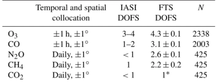
Table 4.Summary of the temporal and spatial collocation crite-ria adopted for each trace gas. Also shown are the typical de-gree of freedom for signal (DOFS) for IASI and FTS products, and the number of coincident observations between IASI and FTS (N). For IASI, the expected DOFS for O3and CO are taken from the Products User Guide (EUM/OPSEPS/MAN/04/0033, EUMET-SAT), while for CH4, N2O, and CO2those are obtained from Tur-quety et al. (2004) and Clerbaux et al. (2009). The FTS DOFS are calculated from the corresponding retrievals between 2010 and 2014 (median±1σ). Note that daily means 24 h means.
Temporal and spatial IASI FTS N collocation DOFS DOFS
O3 ±1 h,±1◦ 3–4 4.3±0.1 2338 CO ±1 h,±1◦ 1–2 3.1±0.1 2003 N2O Daily,±1◦ <1 2.6±0.1 425 CH4 Daily,±1◦ 1 2.2±0.2 425 CO2 Daily,±1◦ <1 1∗ 425
∗Scaled to the a priori VMR profile.
timescale signal (annual means) we reconstructed a time se-ries that only considers the fit results obtained for the mean [TC]gasand the seasonal cycle. Then, by subtracting it from the measured time series, we get a de-seasonalised time se-ries, for which we then calculate the annual mean values. Note that for IASI-A and IASI-B consistency study, the bias between both IASI sensors is also calculated. To do so, we directly compare the measured TCs of all the trace gases and compute the median difference of this difference time series. This temporal decomposition has been done on a logarith-mic scale, i.e. our measured time series correspond to the logarithm of the measured TCs of all the trace gases. This ap-proach has two clear advantages in the subsequent IASI–FTS comparison: (i) the [TC]gasvariations on this scale can be in-terpreted as variations relative to the reference mean values (1ln[TC]gas≈1[TC]gas/[TC]gas) and we thereby directly compare the anomalies observed by both remote sensing in-struments, and (ii) the relative differences between IASI and FTS observations can directly be computed as the subtraction of the corresponding variability on the different timescales (note that the temporal decomposition produces values very close to zero, thereby computing the standard relative differ-ences provides very extreme values in some cases).
4.2 Collocation criteria
Figure 2.Row averaging kernels for O3and CH4as observed by IASI-A and FTS instruments, expressed on logarithm scale, for typical measurement conditions at IZO. US is upper stratosphere, MS is middle stratosphere, UTLS is upper troposphere and lower stratosphere, and T is troposphere. Also shown are the total degree of freedom for signal (DOFS), the vertical profile of the cumulative DOFS, as well as the a priori VMR profiles used for the FTS retrievals.
The collocation criteria selected are the result of a com-promise between the spatial and temporal variability of each trace gas and the uncertainties and spatial range covered by the FTS observations and therefore can vary from gas to gas. Appendix B describes in detail the methodology followed to define the optimal coincidence criteria adopted for each trace gas, summarised in Table 4. In summary, we consider all the IASI observations within the box±1◦latitude/longitude
cen-tred at the IZO location (Fig. 1) and pair those IASI and FTS observations taken within±1 h for O3and CO, and we pair daily median observations corresponding to the same day for the rest of trace gases. As previously mentioned, we con-sider all the TC observations disseminated in V5: Septem-ber 2010–SeptemSeptem-ber 2014 for IASI-A and DecemSeptem-ber 2012– September 2014 for IASI-B. From this data set we only work with the best quality IASI L2 V5 measurements: over sea, cloud free, and with the highest level of quality and com-pleteness of the IASI retrieval as indicated in the Products User Guide (EUM/OPSEPS/MAN/04/0033, EUMETSAT).
For the consistency study between both IASI sensors (IASI-A and IASI-B) the 2◦square has been divided in boxes
of±0.25◦. Moreover, we distinguish between daily morning
(10:00–11:00 UTC) and daily evening (22:00–23:00 UTC) TC observation overpasses in order to carefully analyse a possible bias for each overpass. Then, we compare TC amounts from each overpass and sensor for the same day. Note that for this study the IASI observations are paired with-out forcing temporal coincidence with the FTS data.
4.3 Vertical sensitivity
The vertical sensitivity of a remote sensing spectrometer depends, among other things, on the geometry of observa-tions, the target gas considered as well as the specific char-acteristics of each instrument (e.g. the signal to noise ra-tio, spectral resolution). Hence, the responses of IASI and FTS to real atmospheric variability are significantly
differ-ent. This fact can be observed in Fig. 2, where the rows of the IASI and FTS averaging kernels (A) are displayed for O3and CH4. The IASIAare not operationally dissem-inated in V5; therefore, to illustrate its vertical sensitivity, we have taken the O3 A from the EUMETSAT/IASI L2 version 6 products (EPS Product Validation Report: IASI L2 PPF v6, EUM/TSS/REP/14/776443 v4C, EUMETSAT), while the IASI CH4Ahave been obtained in the framework of the European project MUSICA (Schneider et al., 2013). Note that the rows of A describe the altitude regions that mainly contribute to the retrieved VMR profile and there-fore these kernels can be used to identify the independent layers without significant overlap with other layers. Indeed, the trace ofA(so-called the degrees of freedom for signal, DOFS) is a measure of the number of independent layers re-trieved from the remote sensing measurements. Also, Fig. 2 includes the vertical profiles of the cumulative DOFS, calcu-lated from the top of the atmosphere to surface for IASI and inversely for FTS as well as the a priori VMR used for the FTS retrievals in order to compare with the vertical sensitiv-ity of the two remote sensing instruments.
be sensitive to the maximum O3concentrations in the Chap-man layer and to the tropopause/upper troposphere regions (DOFS∼2.5). The expected IASI DOFS and the obtained FTS DOFS for all the trace gases are also listed in Table 4. The second important fact is that IASI has a weak sensitivity in the lower troposphere for the trace gases considered in this study, leading to the variability of the partial columns missed by FTS below 2373 m a.s.l. (IZO altitude) not being crucial for the IASI–FTS comparison.
5 Consistency between IASI-A and IASI-B observations
In order to probe the continuity provided by IASI-B as well as the consistency of each individual IASI sensor, it is indis-pensable to first analyse the temporal stability of their ob-servations. For this purpose, we examine possible drifts and discontinuities in the times series of the differences between the de-seasonalised variability from IASI-A and IASI-B av-eraged on a weekly basis. The drift is defined as the linear trend in the differences, while the change points (changes in the weekly median of the difference time series) are analysed by using a robust rank order change-point test (Lanzante, 1996; O. E. García et al., 2014). By using these tools, we observe that the time series of the differences between the observations from the morning and evening overpasses for each IASI sensor as well as between the observations from the two sensors for each overpass are homogenous for all the trace gases considered (i.e. no change points were detected at 95 % confidence level). Moreover, all the difference time se-ries reveal no significant drifts at 95 % confidence level. Fig-ure 3 shows the time series of O3TC as observed by IASI-A and IASI-B and the corresponding differences.
This temporal stability study is complemented by analysing whether the distributions of the A and IASI-B observations could be statistically considered equivalent. To do so, we have used the Friedman non-parametric test, which detects differences in the distributions of related vari-ables by checking the null hypothesis that multiple dependent samples come from the same statistical population (Saw-ilowsky and Fahoome, 2005). By applying this test on the observed short-term variability time series from the two IASI sensors for each overpass, which can be considered as four related samples for each trace gas, we only observe signifi-cant differences for the O3distributions between evening and morning overpasses (at 95 % confidence level). Nonetheless, these discrepancies disappear when comparing the observa-tions for the same overpass; therefore, the IASI sensors dis-tinguish the O3 intra-day concentration variations. Indeed, for this trace gas the agreement between both sensors for the same overpass is significantly better than between the two overpasses for each sensor, as observed in Fig. 4, which dis-plays the scatter plots between the O3 trended and
de-Figure 3.Time series of O3TC amounts (in 1×10²²molec m−2) from the IASI-A and IASI-B overpasses (morning, M, and evening, E) (upper panel) and of the differences between the cor-responding de-seasonalised variability (in %) for the morning and evening overpasses (middle and bottom panels). The solid lines rep-resent the difference time series averaged on a weekly basis. The ar-rows distinguish the IASI-B commission mode (from 19 December 2012 to 18 June 2013) and the IASI-B operational mode (from 19 June 2013 onwards).
seasonalised variability as observed by the two IASI sensors for each overpass.
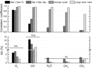
All of these findings suggest that, on the one hand, the ob-servations from each sensor are consistent with themselves and, on the other hand, both sensors similarly reproduce the atmospheric composition variations. The statistics for the IASI-A and IASI-B intercomparison are summarised in Fig. 5 (Pearson correlation coefficient and standard deviation of the de-trended and de-seasonalised differences, and me-dian bias). In summary, we observe that both IASI sensors similarly reproduce the annual cycle of all the trace gases considered (R >0.95 except for CO2, for which we ob-serve a poorer agreement,R∼0.70–0.85), while for the very
short-term concentration variations we find a large correla-tion for O3(∼0.80) and moderate for the rest of trace gases
(R∼0.30–0.60). The scatter (1σ) of the differences among
Figure 4. Scatter plots of the de-trended and de-seasonalised variability (in %) from the IASI-A and IASI-B overpasses (morning and evening) for O3. The legend shows the Pearson correlation coefficient,R, and the colour bar indicates the number of coincident data per bin. The dashed lines represent the diagonals (x=y).
Figure 5.Pearson correlation coefficient (upper panel) between the observations from IASI-A and IASI-B overpasses (morning, M, and evening, E) for all the trace gases considered at different timescales: single measurements (de-trended and de-seasonalised variability, Det+Des) and annual cycle (AC). Middle panel shows the same, but for the standard deviation (in %) of the corresponding differ-ences, while the bottom panel displays the median bias (in %). The number of coincident observations is 675.
CO and between 0.4 and 0.6 % for N2O and CH4 are re-markable (bottom panel in Fig. 5). For O3and CO2the bias is lower than 0.2 % in absolute value.
6 Comparison between IASI and ground-based FTS observations
This section presents the IASI–FTS comparison at differ-ent timescales: single measuremdiffer-ents, daily, annual, and long-term trends. An example of this strategy is displayed in Fig. 6 for O3, while the summary of the intercomparison results for all the trace gases is shown in Fig. 7 (Pearson correlation co-efficient and standard deviation of the differences between IASI and FTS products). The consistency between both IASI sensors has been documented in the previous section. There-fore, here we only focus on IASI-A since it has the longest time series of measurements (September 2010–September 2014 for V5) as well as to ensure a homogeneous sampling during the whole period analysed.
As observed in Fig. 7, IASI reproduces the ground-based FTS observations well at the longest temporal scales, i.e. an-nual cycles and long-term trends. For the latter the correla-tion is larger than 0.95 for all the trace gases with the ex-ception of CO2 (R∼0.70), while on an annual basis, the
Figure 6.Summary of the IASI-A and FTS comparison for O3:(a, b)time series of the TC amounts (in 1×10²²molec m−2) and the de-trended variability (in %) respectively;(c)averaged annual cycle;(d, e)time series of the de-trended+de-seasonalised variability (in %), and the difference between coincident de-trended+de-seasonalised variability from IASI-A and FTS (in %) respectively; and(f)scatter plot of the de-trended+de-seasonalised variability. For(c)and(f)the Pearson correlation coefficient is included in the legends and for(e)the standard deviation of the differences. The number of coincident measurements is 2338.
Figure 7. Pearson correlation coefficient (upper panel) be-tween IASI-A and FTS observations for all the trace gases considered at different timescales: single measurements (de-trended+de-seasonalised variability within±1 h, Det+Des 1 h), daily (de-trended+de-seasonalised variability within the same day, Det+Des Day), annual, and long-term trend. The number of coin-cident data is 2338 for O3, 2003 for CO, and 425 for N2O, CH4, and CO2. Bottom panel shows the same, but for the standard deviation (in %) of the corresponding differences. The solid black lines repre-sent the day-to-day variability calculated from the FTS observations at IZO between 2010 and 2014.
the IASI L2 processor which has not been specifically opti-mised for CO2, since the middle infrared FTS CO2products have successfully proven their reliability to monitor the CO2 concentrations (Barthlott et al., 2015). In particular, the IASI CO2retrieval is solely based on the IASI measurements un-like in Crevoisier et al. (2009a), where collocated microwave measurements are exploited together with IASI data to dis-entangle the temperature and the CO2 signals in the thermal infrared spectra.
For the shortest-term variations we find poorer agree-ments, although the correlation is significantly larger for O3 (∼0.80), but not for the rest of trace gases (R∼0.10–
0.30). When comparing daily values for CO the agreement improves (R∼0.50), suggesting that the IASI sensor could
moderately capture the day-to-day concentration variations but not the intra-day variability. The scatter (1σ) of the
Figure 8.Multi-annual averaged annual cycle for CO, N2O, CH4, and CO2from IASI-A and FTS observations.
2013). Note that IASI–FTS comparison also confirms the re-sults observed for the consistency study of A and IASI-B sensors. The correlations and the scatter of the differences observed for both analysis are very similar both at short-term and intra-annual timescales (recall Figs. 6 and 8) with the ex-ception of CO2. For this trace gas the consistency study re-veals a moderate agreement between both IASI sensors (cor-relations between 0.6 and 0.8 for the annual cycles), but we do not document any agreement for the IASI–FTS compari-son (correlation less than 0.2). This is likely due to the degree of maturity of the IASI CO2 products, as aforementioned. Therefore, the continuous intercomparison of both IASI sen-sors could successfully be used as a quality control for iden-tifying inconsistencies or instrumental issues in lack of ref-erence ground-based observations.
The differences between the IASI and FTS short-term variability have been analysed as a function of the different parameters, such as the relative horizontal distance between IASI footprints and FTS location, or of the different view-ing geometry of the two remote sensview-ing instruments, with-out identifying significant patterns. As example, the study of viewing geometry is displayed in Fig. 9, where we observe that the differences are uncorrelated to the viewing geometry (A air mass (Liou, 1980) and difference between IASI-A and FTS IASI-AMS). Only the differences for O3are displayed as example. However, the same behaviour has been observed for all the trace gases considered.
In addition, the strategic location of IZO allows us to ad-dress the IASI–FTS comparison for different atmospheric
Figure 9. (a) Differences between the O3 trended and de-seasonalised variability time series from IASI-A and FTS (in %) as a function of the IASI-A air mass (AM) plotted as black squares with error bar (median and standard deviation per bins of 0.1 of AM), and simultaneous 2-D plot showing the difference between the IASI-A and FTS AMS.(b)Same as(a)but versus the aerosol optical depth (AOD) at 500 nm, recorded at AERONET SCO station during summer. Also, the differences between IASI-A and IASI-B are included. The black and white squares represent the median and standard deviation per bins of 0.025 of AOD for the IASI-A–FTS and IASI-A–IASI-B differences respectively.(c)Same as(b)but during winter.
affected by the range of the aerosol load, increasing (absolute value) as the corresponding AOD values increase. This pat-tern is likely due to the different type of observations: while the FTS measurements are performed from the ground in the direct solar path, the IASI sensors record thermal emission of the Earth–atmosphere from the space and could be more af-fected by aerosol signatures (thermal emission and scattering processes) (e.g. Vandenbussche et al., 2013; Peyridieu et al., 2013, and references therein). Indeed, when comparing the observations from the two IASI sensors (also displayed in Fig. 9) this difference disappears, which is expected given the very good spectral and radiometric consistency of the two instruments. However, in winter, the IASI–FTS differ-ences seem to be independent on AOD. This fact is likely due to the limited sensitivity of IASI to the boundary layer because of decreasing thermal contrast between the surface and the atmosphere when approaching the surface. In addi-tion to the Saharan condiaddi-tions, we have also analysed the IASI–FTS comparison under polluted air masses likely com-ing from North America or Europe (Cuevas et al., 2013, and references therein) by using the intra-day CO concentration variations from the GAW (Global Atmospheric Watch) in situ observations recorded at IZO as a tracer (see Appendix B for details about GAW programme at IZO). No significant patterns were observed (data not shown), but further analy-sis and longer time series are needed to extract more robust conclusions.
Until now, the IASI–FTS comparison has been addressed in terms of relative variability, but a comparison of absolute TC amounts also provides us useful information. Therefore, to roughly estimate possible biases between IASI-A and FTS observations, the partial column amounts below IZO alti-tude, computed from the WACCM climatological data, have been added to the FTS observations. By using those data, we find that the IASI observations are consistently lower than FTS observations for all the trace gases, with a me-dian bias (IASI–FTS) of ∼ −6 % for O3 and CH4 (−6.4
and −5.9 % respectively) and ∼ −12 % for N2O and CO2 (−12.4 and −12.1 % respectively), except for CO. For CO
we observe the contrary behaviour; i.e. the IASI sensor over-estimates the FTS observations by ∼15 % (15.2 %). These discrepancies could be partly attributed to systematic IASI and FTS error caused, for example, by the lower IASI sen-sitivity to the lower troposphere, uncertainties in the IASI ANNs training procedure or in the spectroscopic line pa-rameters. As previously mentioned in Sect. 3, the errors in the spectroscopic line parameters could explain between 2 and 4 % of the FTS bias, according to our error estima-tion (see Appendix B). Indeed, experimental intercompar-isons between FTS and Brewer observations carried out at IZO in the last years found that FTS systematically over-estimates the Brewer O3 TC amounts by∼4 % (Schneider et al., 2008; Viatte et al., 2011; García et al., 2012b), which may be due to inconsistencies in the ultraviolet and infrared spectroscopic parameters. This implies that the IASI O3
ob-servations should have less bias with respect to the actual O3 concentrations (less than 2 %). However, for CO, the bias ob-tained is likely introduced by the WACCM estimation since previous studies comparing to other space-based CO prod-ucts, like the MOPITT sensor (August et al., 2012), or to dedicated IASI CO retrievals, like the FORLI-CO algorithm (Kerzenmacher et al., 2012), found biases lower than 7 % for regions with low background CO concentrations such as the Atlantic Ocean.
7 Conclusions
This paper documents, for the first time, the uncertainty and the long-term consistency of all EUMETSAT/IASI trace gas products at the same time and using a unique measurement technique as reference, the ground-based FTS experiment.
Firstly, we show that the EUMETSAT/IASI trace gas ob-servations, from both Metop-A/IASI and Metop-B/IASI, are consistent; i.e. neither drifts in time nor were biases found. Therefore, the observations from both remote sensing instru-ments could be merged to obtain a unique IASI database. Secondly, we focus on the IASI versus ground-based FTS measurement comparison. IASI adequately captures the day-to-day TC variation, the annual cycle, and the long-term trend for its operational products O3and CO, as compared to ground-based FTS measurements. Likewise, for N2O and CH4 (trace gases with a rather small day-to-day variabil-ity), IASI observations can successfully be used to describe their seasonality and interannual trend. However, for CO2 an acceptable agreement is only achieved at the long-term scale. For the latter three gases, disseminated as aspirational products, improvements in the EUMETSAT retrieval rithms are currently being carried out to include mature algo-rithms from the wider scientific community. FORLI-CO and FORLI-O3are also being included in the operational IASI L2 suite (Clerbaux et al., 2009). The same methodology can be applied to the upgraded products to support their moni-toring in the long term and in view of the expectation of a continued data record from IASI on Metop-C.
This consistency and quality assessment has been carried out using the ground-based FTS located at the IZO and, thus, it is valid for the subtropical North Atlantic region under free troposphere conditions. Although this quality documen-tation can be used as a benchmark for studies that apply EU-METSAT/IASI trace gas products in climate research, further comparison studies covering other regions might be desirable in order to analyse the possible impact of latitude or other environments, such as urban-industrial or biomass burning areas, on the IASI products accuracy.
Appendix A: Theoretical error estimation of the FTS products
Theoretically, the error of the different FTS products can be estimated by following the formalism detailed by Rodgers (2000), where the difference between the retrieved state,xˆ, and the real state,x, can be written as a linear combination of the a priori state,xa, the real and estimated model param-eters,bandbˆrespectively and the measurement noiseǫ:
(xˆ−x)=(A−I)(x−xa)+GKb(b− ˆb)+Gǫ, (A1)
whereGrepresents the gain matrix,Kba sensitivity matrix to
model parameters,Ithe identify matrix, andAthe averaging kernel matrix.Arelates the real variability to the measured variability of the considered atmospheric state and, thus, rep-resents the way in which the remote sensing system smoothes the real vertical profiles (Rodgers, 2000). Therefore, Eq. (A1) defines three types of error: the first term is the smoothing er-ror associated with the limited vertical sensitivity of the FTS instruments, the second one represents the errors due to un-certainties in the input/model parameters (instrumental char-acteristics, spectroscopy data), and the third one corresponds to the measurement noise).
The theoretical error estimation strongly depends on the assumed uncertainties. In our case, we consider the error sources and values listed in Table A1 for the input param-eters, which are the leading error sources affecting the dif-ferent FTS products, identified from our experience and the literature (Schneider and Hase, 2008; Sepúlveda et al., 2014, and references therein), while the smoothing error is calcu-lated as (A−I)Sa (A−I)T, where Sa matrix is the is the
covariance matrix of the target gas. Strictly, to estimate the smoothing error contribution, the covariance matrix of a real ensemble of atmospheric states must be known (Rodgers, 2000). However, due to lack of real observations of the verti-cal profiles of all the trace gas considered at IZO, theSafor
each target gas is assumed and calculated from the WACCM-V6 model estimates. WACCM is a global chemistry model of well-recognised prestigious that has widely demonstrated its ability to provide reliable estimations of the vertical pro-files of trace gases and their expected concentration varia-tions (Pan and Brasseur, 2006; SPARC Report, 2010; Smith et al., 2011; Brakebusch et al., 2013). Therefore, here theSa
is calculated considering the variance of the corresponding gas concentrations at each altitude from the WACCM-V6 climatological data and a Gaussian distribution of strength 5 km for the inter-layer correlation. Note that the total error values are calculated as the root sum squares of all the er-ror sources considered, where the contribution of each erer-ror source has been split into statistical and systematic contribu-tions. The exceptions are the spectroscopic parameters and the measurement noise, which are considered as purely sys-tematic and statistical respectively. This error estimation has been applied to the IZO FTS observations between 2010 and 2014 (period studied in the current work).
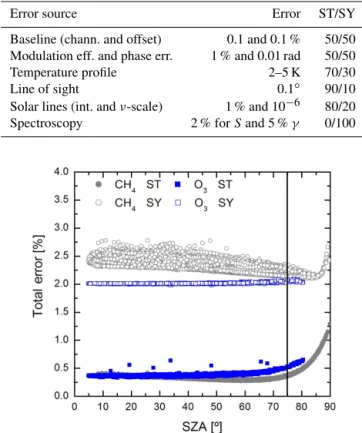
Table A1.Error sources used for the theoretical error estimation for all the FTS products (chann.: channeling; eff.: efficiency; err.: error; int.: intensity;ν-scale: spectral position;S: intensity;γ: pressure broadening parameter). The second column gives the assumed error value and the third column the partitioning of this error between statistical (ST) and systematic (SY) contributions (Sepúlveda et al., 2014).
Error source Error ST/SY
Baseline (chann. and offset) 0.1 and 0.1 % 50/50 Modulation eff. and phase err. 1 % and 0.01 rad 50/50
Temperature profile 2–5 K 70/30
Line of sight 0.1◦ 90/10
Solar lines (int. andν-scale) 1 % and 10−6 80/20 Spectroscopy 2 % forSand 5 %γ 0/100
Figure A1.Total statistical (ST) and systematic (SY) errors (in %) as a function of the solar zenith angle (SZA, in◦) for FTS O3and CH4measurements between 2010 and 2014. The black solid line represents the limit value of SZA=75◦. Beyond this value the FTS observations are discarded.
The FTS total errors (statistical and systematic) depend on the observing geometry at which FTS observations are car-ried out. As illustrated in Fig. A1, the larger theoretical errors are found at high solar zenith angles (SZAs), mainly due to the fact that the FTS observations are more sensitive to possi-ble misalignments of the solar tracker at these SZAs. There-fore, these data (SZA>75◦) are excluded from the study to
avoid unrealistic FTS retrievals in the FTS-IASI intercom-parison, which represent between 1 % for CO and 8 % for N2O, CH4, and CO2. Considering the filtered FTS obser-vations, the total statistical errors (medians and ±1σ) are
and the phase error) dominate the statistical errors for the stratospheric gas O3. For all the target gases, the systematic error budget is lead by the spectroscopic errors, with me-dian values and±1σ of 2.00±0.01 % for O3, 2.10±0.04 %
for CO, 2.10±0.01 % for N2O, 2.35±0.01 % for CH4, and 3.50±0.04 % for CO2.
Appendix B: Collocation criteria between IASI and ground-based FTS observations
To define the temporal collocation, we first estimate the intra-day concentration variations of the target gases and, then, analyse whether the FTS system is good enough to detect this variability by comparing to the respective FTS uncer-tainties. To do so and to be independent from the FTS ob-servations, we use the high-frequency and high-quality data routinely measured by different in situ analyzers and Brewer spectrometers at IZO.
Ground-level in situ atmospheric continuous measure-ments of CO2 (since 1984), CH4 (since 1984), CO (since 2008), and N2O (since 2007) have been routinely carried out at IZO as a contribution of AEMET to the WMO GAW programme (Cuevas et al., 2015). The high qual-ity of these measurements has been externally assessed by (1) periodic audits performed in 2004 (CH4), 2008 (N2O; Scheel, 2009), 2009 (CO, CH4, and N2O; Zell-weger et al., 2010, and references therein), and 2013– 2014 (CO, CH4, CO2, and N2O, report in preparation) by the World Calibration Centre for Surface Ozone, Carbon Monoxide, Methane and Carbon Dioxide (WCC-Empa), and the World Calibration Centre for Nitrous Oxide (WCC-N2O); (2) the participation in WMO Round Robin in-tercomparisons (e.g. WMO Round Robin 5, www.esrl. noaa.gov/gmd/ccgg/wmorr/wmorr_results.php); and (3) the continuous comparison to simultaneous weekly discrete data (Gómez-Peláez et al., 2012, 2013) obtained by the NOAA analysis of weekly collected flask samples, within the NOAA/ESRL/GMD CCGG cooperative air sampling network (www.esrl.noaa.gov/gmd/ccgg/flask.php). The ex-pected uncertainties in these IZO continuous atmospheric measurements are ±0.1 ppm for CO2, ±2 ppb for CH4, ±0.2 ppb for N2O, and ±2 ppb for CO. Refer to Gómez-Peláez and Ramos (2011), Gómez-Gómez-Peláez et al. (2012) and Gómez-Peláez et al. (2013) for more details about the mea-surements and the techniques used. Regarding O3, we use the daytime O3TC observations performed by Brewer spec-trometers at IZO since 1991. Like the FTS measurements, the Brewer O3data are part of NDACC since 2001. Furthermore, since 2003 they are the Regional Brewer Calibration Center for Europe (www.rbcc-e.org) of the WMO GAW. This guar-antees the high quality of their measurements (better than 1 %; Redondas et al., 2014, and references therein).
The intra-day concentration variations have been esti-mated through the intra-day variation coefficient (VC),
cal-Figure B1.Intra-day variation coefficient (VC) for O3total column and in situ CH4(in %]) as observed by a Brewer spectrometer and a GAW in situ GC-FID analyzer respectively between 2008 and 2013. The solid and dashed black lines represent the median and±1σ of the reference intra-day VC respectively, and the dashed red lines represent the range of theoretical and experimental FTS errors.
Figure B2.Horizontal distance covered by the FTS observations (in km) versus the solar zenith angle (SZA; in ◦), at which they are taken for all the target gases. The dashed lines represent the maximal horizontal distances.
As for the temporal collocation, the spatial coincidence criteria have to take into account the spatial concentration variations of each trace gas and the maximal horizontal dis-tance covered by the FTS observations. Since the FTS mea-surements are performed in the direct solar path, the hori-zontal projection of the air masses probed by the FTS can be easily calculated from the actual solar observing geometry and the effective altitude of the vertical column observed by the FTS. The latter has been defined as the altitude at which 95 % of the corresponding TC amount is observed and, thus, varies from gas to gas. These effective altitudes have been de-termined by using the WACCM-V6 climatological data and are∼40 km for O3and∼20 km for the rest of gases, result-ing in a maximal horizontal distance of∼150 km for O3and ∼80 km for the rest of gases (see Fig. B2).
Regarding the spatial concentration variations of each trace gas, we should consider that IZO is far away from the target gas sources/sinks and embedded in the free tropo-sphere, thereby usually affected by long-range transports of aged and well-mixed air masses (e.g. Cuevas et al., 2013, and references therein). In addition, the latitudinal/longitudinal gradients of the trace gases considered here are rather smooth at oceanic subtropical latitudes. Indeed, the latitudinal rel-ative difference of CO2 between the Equator and 60◦N in 2012 was smaller than 2.5 % (WDCGG, 2014), leading to a mean CO2 gradient smaller than 0.04 % per degree of lat-itude. For CH4 and CO, the latitudinal relative difference between the means of the latitudinal bands 0–30 and 30– 60◦N in 2012 was smaller than 3.8 and 40 % respectively
(WDCGG, 2014). This implies mean CH4and CO gradients smaller than 0.13 and 1.3 % per degree of latitude respec-tively. In the previous three gradient estimations, we have also taken into account the seasonal cycles, which depend on latitude (i.e. we are not simply considering the annual mean latitudinal gradients). For N2O, the latitudinal relative differ-ence between 20 and 40◦N is smaller than 0.32 % (Huang
et al., 2008; Kort et al., 2011) and the seasonal cycle is in-significant as can be seen in WDCGG (2014). This implies a mean N2O gradient smaller than 0.016 % per degree of latitude. For O3a gradient of 0.92 % per degree of latitude could be expected at the IZO latitude (value obtained from the ozone observations in 2012 of the space-based Ozone Monitoring Instrument (OMI); Veefkind et al., 2006). There-fore, assuming constant latitudinal gradients within the box ±1◦latitude/longitude centred at IZO, the spatial
concentra-tion variaconcentra-tions inside the box (defined in an equivalent way as the temporal intra-day VC) are expected to be 0.53 % for O3, 0.75 % for CO, 0.01 % for N2O, 0.08 % for CH4, and 0.023 % for CO2(where we have taken into account that the standard deviation, in a segment of length 2◦, of a linear function with
slope Gr per degree, is equal to Gr/√3). These spatial VC
are similar (for O3 and CO) or much smaller (for the rest of trace gases) than the statistical uncertainties of the FTS (recall Table 3). Therefore, no significant concentration vari-ations might be expected within the actual area probed by the FTS observations and, indeed, a slightly wider range than this can be applied for collocating IASI measurements without affecting the validation results. Thus, we define a validation box of±1◦centred at IZO location (i.e.± ∼110 km at IZO
Acknowledgements. The research leading to these results has
re-ceived funding from the Ministerio de Economía y Competitividad from Spain for the project CGL2012-37505 (NOVIA project) and from EUMETSAT under the Fellowship Programme (VALIASI project). Furthermore, M. Schneider, S. Barthlott, A. Wiegele, and Y. González are supported by the European Research Council under FP7/(2007–2013)/ERC grant agreement no. 256961 (MUSICA project).
Edited by: A. Kokhanovsky
References
Alonso-Pérez, S., Cuevas, E., and Querol, X.: Objective identifica-tion of synoptic meteorological patterns favouring African dust intrusions into the marine boundary layer of the subtropical east-ern north Atlantic region, Meteorol. Atmos. Phys., 113, 109–124, 2011.
Angelbratt, J., Mellqvist, J., Blumenstock, T., Borsdorff, T., Bro-hede, S., Duchatelet, P., Forster, F., Hase, F., Mahieu, E., Murtagh, D., Petersen, A. K., Schneider, M., Sussmann, R., and Urban, J.: A new method to detect long term trends of methane (CH4) and nitrous oxide (N2O) total columns measured within the NDACC ground-based high resolution solar FTIR network, Atmos. Chem. Phys., 11, 6167–6183, doi:10.5194/acp-11-6167-2011, 2011.
August, T., Klaes, D., Schlüssel, P., Hultberg, T., Crapeau, M., Arriaga, A., O’Carroll, A., Coppens, D., Munro, R., and Cal-bet, X.: IASI on Metop-A: Operational Level 2 retrievals after five years in orbit, J. Quant. Spectrosc. Ra., 113, 1340–1371, doi:10.1016/j.jqsrt.2012.02.028, 2012.
Barret, B., De Mazière, M., and Mahieu, E.: Ground-based FTIR measurements of CO from the Jungfraujoch: characterisation and comparison with in situ surface and MOPITT data, At-mos. Chem. Phys., 3, 2217–2223, doi:10.5194/acp-3-2217-2003, 2003.
Barthlott, S., Schneider, M., Hase, F., Wiegele, A., Christner, E., González, Y., Blumenstock, T., Dohe, S., García, O. E., Sepúlveda, E., Strong, K., Mendonca, J., Weaver, D., Palm, M., Deutscher, N. M., Warneke, T., Notholt, J., Lejeune, B., Mahieu, E., Jones, N., Griffith, D. W. T., Velazco, V. A., Smale, D., Robinson, J., Kivi, R., Heikkinen, P., and Raffalski, U.: Us-ing XCO2retrievals for assessing the long-term consistency of NDACC/FTIR data sets, Atmos. Meas. Tech., 8, 1555–1573, doi:10.5194/amt-8-1555-2015, 2015.
Blumstein, D., Chalon, G., Carlier, T., Buil, C., Hébert, P., Ma-ciaszek, T., Ponce, G., Phulpin, T., Tournier, B., and Siméoni., D.: IASI instrument: Technical Overview and measured perfor-mances, in: Proccedings SPIE, SPIE, Denver, 2004.
Brakebusch, M., Randall, C. E., Kinnison, D. E., Tilmes, S., San-tee, M. L., and Manney, G. L.: Evaluation of Whole Atmosphere Community Climate Model simulations of ozone during Arc-tic winter 2004–2005, 118, 2673–2688, doi:10.1002/jgrd.50226, 2013.
Brasseur, G., Hauglustaine, D., Walters, S., Rasch, P., J.-F.Muller, Granier, C., and Tie, X.: MOZART: A global chemical trans-port model for ozone and related chemical tracers – Part
1: Model Description, J. Geophys. Res.-Atmos., 103, 28265– 28289, doi:10.1029/98JD02397, 1998.
Clerbaux, C., Boynard, A., Clarisse, L., George, M., Hadji-Lazaro, J., Herbin, H., Hurtmans, D., Pommier, M., Razavi, A., Turquety, S., Wespes, C., and Coheur, P.-F.: Monitoring of atmospheric composition using the thermal infrared IASI/MetOp sounder, At-mos. Chem. Phys., 9, 6041-6054, doi:10.5194/acp-9-6041-2009, 2009.
Crevoisier, C., Chédin, A., Matsueda, H., Machida, T., Armante, R., and Scott, N. A.: First year of upper tropospheric integrated con-tent of CO2from IASI hyperspectral infrared observations, At-mos. Chem. Phys., 9, 4797–4810, doi:10.5194/acp-9-4797-2009, 2009a.
Crevoisier, C., Nobileau, D., Fiore, A. M., Armante, R., Chédin, A., and Scott, N. A.: Tropospheric methane in the tropics – first year from IASI hyperspectral infrared observations, Atmos. Chem. Phys., 9, 6337–6350, doi:10.5194/acp-9-6337-2009, 2009b. Crevoisier, C., Nobileau, D., Armante, R., Crépeau, L., Machida, T.,
Sawa, Y., Matsueda, H., Schuck, T., Thonat, T., Pernin, J., Scott, N. A., and Chédin, A.: The 2007–2011 evolution of tropical methane in the mid-troposphere as seen from space by MetOp-A/IASI, Atmos. Chem. Phys., 13, 4279–4289, doi:10.5194/acp-13-4279-2013, 2013.
Crevoisier, C., Clerbaux, C., Guidard, V., Phulpin, T., Armante, R., Barret, B., Camy-Peyret, C., Chaboureau, J.-P., Coheur, P.-F., Crépeau, L., Dufour, G., Labonnote, L., Lavanant, L., Hadji-Lazaro, J., Herbin, H., Jacquinet-Husson, N., Payan, S., Péquig-not, E., Pierangelo, C., Sellitto, P., and Stubenrauch, C.: Towards IASI-New Generation (IASI-NG): impact of improved spectral resolution and radiometric noise on the retrieval of thermody-namic, chemistry and climate variables, Atmos. Meas. Tech., 7, 4367–4385, doi:10.5194/amt-7-4367-2014, 2014.
Cuevas, E., González, Y., Rodríguez, S., Guerra, J. C., Gómez-Peláez, A. J., Alonso-Pérez, S., Bustos, J., and Milford, C.: As-sessment of atmospheric processes driving ozone variations in the subtropical North Atlantic free troposphere, Atmos. Chem. Phys., 13, 1973–1998, doi:10.5194/acp-13-1973-2013, 2013. Cuevas, E., Milford, C., Bustos, J. J., del Campo-Hernández, R.,
García, O. E., García, R. D., Gómez-Peláez, A. J., Ramos, R., Redondas, A., Reyes, E., Rodríguez, S., Romero-Campos, P. M., Schneider, M., Belmonte, J., Gil-Ojeda, M., Almansa, F., Alonso-Pérez, S., Barreto, A., González-Morales, Y., Guirado-Fuentes, C., López-Solano, C., Afonso, S., Bayo, C., Berjón, A., Bethencourt, J., Camino, C., Carreño, V., Castro, N. J., Cruz, A. M., Damas, M., De Ory-Ajamil, F., García, M. I., Fernández-de Mesa, C. M., González, Y., HernánFernández-dez, C., HernánFernández-dez, Y., Hernández, M. A., Hernández-Cruz, B., Jover, M., Kühl, S. O., López-Fernández, R., López-Solano, J., Peris, A., Rodríguez-Franco, J. J., Sálamo, C., Sepúlveda, E., and Sierra, M.: Izaña Atmospheric Research Center Activity Report 2012–2014, State Meteorological Agency (AEMET), Madrid, Spain, and World Meteorological Organization (WMO), Geneva, Switzer-land, nIPO: 281-15-004-2, WMO/GAW Report No. 219, avail-able at: http://izana.aemet.es, last access: 1 December 2015. Díaz, A. M., Díaz, J. P., Expósito, F. J., Hernández-Leal, P. A.,
Dubravica, D., Birk, M., Hase, F., Loos, J., Palm, M., Sadeghi, A., and Wagner, G.: Improved spectroscopic parameters of methane in the MIR for atmospheric remote sensing, in: High Resolu-tion Molecular Spectroscopy 2013 meeting, 25–30 August 2013, Budapest, Hungary, available at: http://lmsd.chem.elte.hu/hrms/ abstracts/D16.pdf (last access: 1 December 2015), 2013. García, O. E., Díaz, J. P., Expósito, F. J., Díaz, A. M., Dubovik, O.,
Derimian, Y., Dubuisson, P., and Roger, J.-C.: Shortwave radia-tive forcing and efficiency of key aerosol types using AERONET data, Atmos. Chem. Phys., 12, 5129–5145, doi:10.5194/acp-12-5129-2012, 2012a.
García, O. E., Schneider, M., Redondas, A., González, Y., Hase, F., Blumenstock, T., and Sepúlveda, E.: Investigating the long-term evolution of subtropical ozone profiles applying ground-based FTIR spectrometry, Atmos. Meas. Tech., 5, 2917–2931, doi:10.5194/amt-5-2917-2012, 2012b.
García, O. E., Schneider, M., Hase, F., Blumenstock, T., Wiegele, A., Sepúlveda, E., and Gómez-Peláez, A.: Validation of the IASI operational CH4and N2O products using ground-based Fourier Transform Spectrometer: Preliminary results at the Izaña Obser-vatory (28◦N, 17◦W), Ann. Geophys.-Italy, 56, doi:10.4401/ag-6326, 2013.
García, O. E., Schneider, M., Hase, F., Blumenstock, T., Sepúlveda, E., Gómez-Peláez, A., Barthlott, S., Dohe, S., González, Y., Meinhardt, F., and Steinbacher, M.: Monitoring of N2O by ground-based FTIR: optimisation of retrieval strategies and com-parison to GAW in-situ observations, NDACC-IRWG/TCCON Meeting, Bad Sulza, Germany, available at: http://www.novia. aemet.es (last access: 1 December 2015), 2014.
García, R. D., García, O. E., Cuevas, E., Cachorro, V. E., Romero-Campos, P. M., Ramos, R., and de Frutos, A. M.: Solar radiation measurements compared to simulations at the BSRN Izaña sta-tion, Mineral dust radiative forcing and efficiency study, J. Geo-phys. Res., 119, 179–194, doi:10.1002/2013JD020301, 2014. Gisi, M., Hase, F., Dohe, S., and Blumenstock, T.: Camtracker:
a new camera controlled high precision solar tracker sys-tem for FTIR-spectrometers, Atmos. Meas. Tech., 4, 47–54, doi:10.5194/amt-4-47-2011, 2011.
Gómez-Peláez, A. J. and Ramos, R.: Improvements in the Car-bon Dioxide and Methane Continuous Measurement Programs at Izaña Global GAW Station (Spain) during 2007–2009, in: 15th WMO/IAEA Meeting of Experts on Carbon Dioxide, Other Greenhouse Gases, and Related Tracer Measurement Tech-niques, Jena, Germany, 7–10 September, 2009, GAW Report No. 194, 133–138, World Meteorological Organization, Jena, Ger-many, 2011.
Gómez-Peláez, A. J., Ramos, R., Gómez-Trueba, V., Campo-Hernández, R., Dlugokencky, E., and Conway, T.: New improve-ments in the Izaña (Tenerife, Spain) global GAW station in-situ greenhouse gases measurement program, in: 16th WMO/IAEA Meeting on Carbon Dioxide, Other Greenhouse Gases, and Re-lated Measurement Techniques (GGMT-2011), Wellington, New Zealand, 25–28 October 2011, GAW Report No. 206, 76–81, World Meteorological Organization, Wellington, New Zealand, 2012.
Gómez-Peláez, A. J., Ramos, R., Gomez-Trueba, V., Novelli, P. C., and Campo-Hernandez, R.: A statistical approach to quan-tify uncertainty in carbon monoxide measurements at the Izaña
global GAW station: 2008–2011, Atmos. Meas. Tech., 6, 787– 799, doi:10.5194/amt-6-787-2013, 2013.
Hase, F.: Improved instrumental line shape monitoring for the ground-based, high-resolution FTIR spectrometers of the Net-work for the Detection of Atmospheric Composition Change, Atmos. Meas. Tech., 5, 603–610, doi:10.5194/amt-5-603-2012, 2012.
Hase, F., Blumenstock, T., and Paton-Walsh, C.: Analysis of the instrumental line shape of high-resolution Fourier transform IR spectrometers with gas cell measurements and new retrieval soft-ware, Appl. Optics, 38, 3417–3422, 1999.
Hase, F., Hanningan, J. W., Coffey, M. T., Goldman, A., Höfner, M., Jones, N. B., Rinsland, C. P., and Wood, S. W.: Intercomparison of retrieval codes used for the analysis of high-resolution ground-based FTIR measurements, J. Quant. Spectrosc. Ra., 87, 25–52, 2004.
Herbin, H., Hurtmans, D., Clerbaux, C., Clarisse, L., and Co-heur, P.-F.: H162 O and HDO measurements with IASI/MetOp, At-mos. Chem. Phys., 9, 9433–9447, doi:10.5194/acp-9-9433-2009, 2009.
Holben, B., Eck, T., Slutsker, I., Tanré, D., Buis, J., Setzer, A., Vermote, E., Reagan, J., Kaufman, Y., Nakajima, T., Lavenu, F., Jankowiak, I., and Smirnov, A.: AERONET-A Federated In-strument Network and Data Archive for Aerosol Characteri-zation, Remote Sens. Environ., 66, 1–16, doi:10.1016/S0034-4257(98)00031-5, 1998.
Huang, J., Golombek, A., Prinn, R., Weiss, R., Fraser, P., Sim-monds, P., Dlugokencky, E. J., Hall, B., Elkins, J., Steele, P., Langenfelds, R., Krummel, P., Dutton, G., and Porter, L.: Es-timation of regional emissions of nitrous oxide from 1997 to 2005 using multinetwork measurements, a chemical transport model, and an inverse method, J. Geophys. Res., 113, D17313, doi:10.1029/2007JD009381, 2008.
IASI Level 2 Product Guide: EUM/OPSEPS/MAN/04/0033, EU-METSAT, available at: www.eumetsat.int (last access: 1 Decem-ber 2015), 2012.
Keim, C., Eremenko, M., Orphal, J., Dufour, G., Flaud, J.-M., Höpfner, M., Boynard, A., Clerbaux, C., Payan, S., Coheur, P.-F., Hurtmans, D., Claude, H., Dier, H., Johnson, B., Kelder, H., Kivi, R., Koide, T., López Bartolomé, M., Lambkin, K., Moore, D., Schmidlin, F. J., and Stübi, R.: Tropospheric ozone from IASI: comparison of different inversion algorithms and validation with ozone sondes in the northern middle latitudes, Atmos. Chem. Phys., 9, 9329–9347, doi:10.5194/acp-9-9329-2009, 2009. Kerzenmacher, T., Dils, B., Kumps, N., Blumenstock, T., Clerbaux,
C., Coheur, P.-F., Demoulin, P., García, O., George, M., Griffith, D. W. T., Hase, F., Hadji-Lazaro, J., Hurtmans, D., Jones, N., Mahieu, E., Notholt, J., Paton-Walsh, C., Raffalski, U., Ridder, T., Schneider, M., Servais, C., and De Mazière, M.: Validation of IASI FORLI carbon monoxide retrievals using FTIR data from NDACC, Atmos. Meas. Tech., 5, 2751–2761, doi:10.5194/amt-5-2751-2012, 2012.
Kort, E. A., Patra, P. K., Ishijima, K., Daube, B. C., Jiménez, R., Elkins, J., Hurst, D., Moore, F. L., Sweeney, C., and Wofsy, S. C.: Tropospheric distribution and variability of N2O: Evidence for strong tropical emissions, Geophys. Res. Lett., 38, L15806, doi:10.1029/2011GL047612, 2011.