Advances in Mechanical Engineering 2015, Vol. 7(12) 1–17
ÓThe Author(s) 2015 DOI: 10.1177/1687814015619276 aime.sagepub.com
Path planning of mobile robot by
mixing experience with modified
artificial potential field method
Huasong Min, Yunhan Lin, Sijing Wang, Fan Wu and Xia Shen
Abstract
In this article, a new method is proposed to help the mobile robot to avoid many kinds of collisions effectively, which combined past experience with modified artificial potential field method. In the process of the actual global obstacle avoidance, system will invoke case-based reasoning algorithm using its past experience to achieve obstacle avoidance when obstacles are recognized as known type; otherwise, it will invoke the modified artificial potential field method to solve the current problem and the new case will also be retained into the case base. In case-based reasoning, we innova-tively consider that all the complex obstacles are retrieved by two kinds of basic build-in obstacle models (linear obstacle and angle-type obstacle). Our proposed experience mixing with modified artificial potential field method algorithm has been simulated in MATLAB and implemented on actual mobile robot platform successfully. The result shows that the proposed method is applicable to the dynamic real-time obstacle avoidance under unknown and unstructured environ-ment and greatly improved the performances of robot path planning not only to reduce the time consumption but also to shorten the moving distance.
Keywords
Mobile robot path planning, case-based reasoning, modified artificial potential method
Date received: 12 March 2015; accepted: 2 November 2015
Academic Editor: Long Cheng
Introduction
During the past two decade, robotics has been devel-oped rapidly. Many researchers put their attentions on the navigation of mobile robots. The most basic tech-nology of navigation is path planning which is going to find a safe and efficient way from starting point to tar-get. In recent years, research on path planning has focused on local searching in dynamic environments, where the pose and location of the obstacles are unknown or partially unknown.
A well-known approach to localize the path of mobile robots is artificial potential field (APF) method,1which is used commonly in real-time collision avoidance and smooth path for mobile robots because of its elegant mathematical analysis and simplicity.
However, its inherent defects are obvious. First, Robot cannot reach the target nearby the obstacle. The obsta-cle repulsion increases and gravity decreases rapidly when target point is within the influence scope of obstacle. Second, there is a local minimum problem; when robot is in the process of traveling, the direction
Engineering Research Center of Metallurgical Automation and Measurement Technology, Ministry of Education, Wuhan University of Science and Technology, Wuhan, China
Corresponding author:
Huasong Min, Engineering Research Center of Metallurgical Automation and Measurement Technology, Ministry of Education, Wuhan University of Science and Technology, No. 947, Heping Avenue, Wuhan, Hubei 430081, China.
Email: [email protected]
of total force and the movement direction of planning path are on the same straight line, and robot cannot avoid obstacle effectively but vibrates back and forth in a certain range. A lot of researchers have proposed some improvements on the traditional APF method in recent years. In 2003, MC Lee and Park2proposed an improved APF method using a virtual obstacle con-cept. A virtual obstacle is located around local mini-mums to repel the mobile robot. This method is adaptable for a real-time path planning because of its lower complexity. However, it is not suitable for the discrete modeling of the mobile robot in complex situa-tion. In 2009, S Charifa and Bikdash3 presented an adaptive boundary following algorithm guided by APF to avoid the local minima. When the size of obstacles is large, too much computing time need to be taken to guide the robot. In 2011, Q Li et al.4 improved the APF method by providing an additional force and developing the virtual local minimum. The genetic algorithm was introduced to optimize the parameters such as the revolved angle of repulsion. The proposed method could plan out a simple, smooth, and safe path by simulation experiments, but not be applicable to the real world. In 2012, L Guan-chen et al.5 integrated APF approach with receding horizon control method. An additional control term was added in path planning to escape from local minima of APF. This term accom-plishes the description of specified property index except for distance and control energy, but the compu-tational process is complicated. In the same year, Q Song and Liu6presented a dynamic fuzzy APF method to overcome the shortcomings of APF method. Through taking the advantage of velocity vector, modi-fying the potential field force function, and integrating with the fuzzy control method, all those steps could achieve adjusting the factors of repulsion potential field in real time. However, inputting the fuzzy control method increases the planning time greatly, and in practical applications, the impact of acceleration should be considered.
Moreover, several artificial intelligence algorithms such as fuzzy logic,7 neural networks,8 and genetic algorithm9 have been proposed for the mobile robot navigation problem in unknown environments. The varied information of the environment needs to be detected by sensors to help the robot avoid obstacles autonomously. Those algorithms could achieve optimal local path planning, but they are relatively complex, time-consuming, and not very useful for real-time applications.
In fact, one of the main issues for mobile robot to navigate in uncertain environment is the lack of prior information. If environmental information could be acquired before path planning, it would contribute to guide the robot moving from the starting point to the target. Case-based reasoning (CBR)10 is a technique
that can reuse previous experience to obtain the suitable information to solve the current problems. Actually, CBR has been used in robotics to perform different tasks for many years. In 2003, Kruusmaa11 presents a global navigation strategy for autonomous mobile robots in dynamic environments. CBR is used to store those solutions and their outcomes for a later use. It can improve the performance of the robot in a difficult uncertain environment, while is not efficient in simple dynamic environments. Moreover, the restrictions of this approach are that the size of the environment and the position of the goal points have to be known pre-cisely, and the localization errors have to be small (just like it is with outdoor applications with global position-ing system (GPS)). Urdiales et al.12in 2006 proposed a sonar-based purely reactive navigation technique for mobile platforms which was relied on CBR algorithm. CBR is used here to let a robot learn how to react in any given situation, so that it can adapt itself to any configuration or environment. However, this system is a purely reactive scheme, its case base can only be trained and learnt by human intervention or other high-level planner system in advance to realize autonomous path planning and does not have the ability to self-learning by its own build-in basic case base. Hoda´l and Dvorˇa´k13 in 2008 combined CBR with graph algo-rithms, which is represented by a rectangular grid. It is applicable to the large-scale environments, saving com-puting time and traveling distance; nevertheless, the process is too complex to reduce the efficiency of the algorithm. To sum up, CBR technique can improve the performance of path planning for mobile robots in complicated environments, while the efficiency and applicability are different when CBR has been used in different platforms.
physical environment. Finally, we summarize the con-clusion and future plan.
‘‘EMMAPF’’ method
In this section, a detailed description of ‘‘EMMAPF’’ method is represented, including the modified APF method and CBR technique. By retrieving and adapt-ing past problems from the case base, we can obtain the solution for current problem; this method can not only help the robot to avoid the obstacles autonomously but also save the computing time and traveling distance to obtain an optimal path.
The procedure of ‘‘EMMAPF’’ method is shown as above (Algorithm 1).
When the existence of obstacles around the robot is detected by sensors, some related information would be returned to system. After sorting and calculation, it will retrieve the similar cases from the case base based on those attribute datum. If the returned solutions are more than one, select the closest case, and then reset the transferring direction. Otherwise, the system will invoke the ‘‘MAPF’’ method. Finally, evaluate the pro-posed solution by the costr(Pp) and update the system by learning from the case base. Thus, in CBR system, learning and adaptation are through accumulation of cases.
‘‘MAPF’’ method
The traditional APF method is commonly used in real-time obstacle avoidance and smooth path for mobile
robots. It is particularly attractive because of its elegant mathematical analysis and simplicity. However, there exists a local minima problem, and no optimization process is involved. Liu et al.15have proposed a concept of virtual obstacle to solve this problem. The virtual obstacle is located around local minimums to repel the mobile robot. We make some improvements based on this approach, modify the potential field force function, and set the virtual obstacle according to the shapes of obstacles detected by the sensor. The steps are shown as follows.
Modify the potential field force function. The attractive force function is described in formula (1)
Fattð ÞX = grad U½ attð ÞX =k X Xgoal
ð1Þ
where k is the attractive force factor and (X Xgoal)
represents the distance from robot to the target. The repulsive force functions are described in formu-las (2)–(5)
Frep=Frep1+Frep2 ð2Þ
Frep1=h
1
r
1
r0
1
r2 X Xgoal
n
ð3Þ
Frep2= n
2h 1
r
1
r0
2
XXgoal
n1
ð4Þ
Frep= Frep
1+Frep2 rr0
0 r.r0
ð5Þ
Algorithm 1:‘‘EMMAPF’’ algorithm.
When the sensors have detected the obstacle { Return the relevant information about the obstacle
Retrieve the similar case from the case base by usingnearest neighbor method. Ifthere is a similar case/are similar cases in the case base
{Return the similar case/cases. If number of the returned cases is greater than one. Revisethe cases to find the most similar caseCp.
Accept the solutionSpofCp {Reset the transferring direction.
Calculate the cost r(Pp).It stands for the speed of the robot using CBR to avoid the obstacle.} }
Else
{Invoke the ‘‘MAPF’’ method to solve the current problem. Find the solutionSmto avoid the obstacle. Calculate the cost r(Pp).It stands for the speed of the robot using ‘‘MAPF’’ method to avoid the obstacle. }
Case learning
{Ifthere is no similar case in the case base. {Store the new case, its solution, andr(Pp)} Else
{ ifr(Pp)\r(Ppold) {Updater(Pp)} }
wherer is the shortest distance between the position of the robot and obstacle,r0is the radius of obstacle sphere of influence,hrepresents the repulsive factor, andnis a real number greater than zero. Contrast with the original potential field function, it introduces the relative distance between the target and the robot (XXgoal), ensuring
the whole potential field minimum only existing at the target point Xgoal. Thus, the gravitational potential field
is always greater than the repulsive potential field, till the robot reaching the target point, the potential field of gravity and repulsive then reduced to zero.
The total force is described in formula (6)
Fall=Fatt+
Xm
1
Frep ð6Þ
wheremis the quantity of the obstacles. The total force will help system to solve the target non-reachable prob-lem with obstacle nearby.
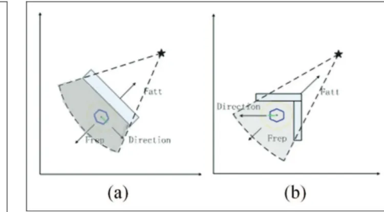
Set the virtual potential field area. While the robot gets trapped in a local minimum, it will stop there or repeat the same route back and forth in a certain range. There are two cases of local minimum shown in Figure 1.
In 2009, Dr Lei16 proposed a new method which increases a special virtual potential based on the origi-nal repulsion field to solve this problem. They used a combination method to push the robot away from the local minima. Based on this method, we set the virtual potential field area as the shaded part in Figure 2. When the robot encounters the local minima, take the target point as the center, and calculate the radiusRby equation (7) as the virtual potential field area
R=max distance Xobs1,Xgoal
,distance Xobs2,Xgoal
+r0
ð7Þ
where Xgoal represents the target point, Xobs1 and Xobs2
represent the endpoints of the obstacle, and r0 is the
influence distance of the obstacle. During this part, the robot travels along the border of the obstacle. Figure 2 shows the effect of the modified APF method. Until the robot travels out of the shaded area, the virtual poten-tial field area will be revoked.
CBR technique
CBR is a self-learning method which helps to solve the current problem by re-using past cases and experiences to adapt to the changes in the environment. This method is based on the concept that similar problems have similar solutions. The innovation of our proposed CBR algorithm is that the cases of complex obstacles can be retrieved by two basic build-in case models which composed of ‘‘linear obstacle model’’ and ‘‘angle-type obstacle model.’’ Three steps can represent a sim-plified description of our CBR technique: retrieving the most similar case or cases, revising the proposed solu-tion, and learning and retaining the new case for future problem solving. The flowchart of CBR technique is shown in Figure 3.
Case representation. When using CBR technique to achieve path planning for mobile robots, the first fun-damental decision to be made is how to establish a case base. Cases can be stored in many different representa-tional formats,17 such as framework representation, object-oriented representation, and predicate represen-tation. Because of its features of applicability, summar-izing, structuring, and reasoning, we choose framework as the representational format. A classical case base usually includes characteristic of the problem and the relevant solution that was used on an earlier occasion when a similar situation was encountered. A case can be described as follows
CaseBase=hC1,C2,C3,. . .,Cii ð8Þ
C=hF,Si ð9Þ
Figure 1. Two cases of local minimum: (a) local minimum case 1 and (b) local minimum case 2.
whereF represents the features of the obstacle andS
represents the relevant solution
F=hcaseID,obstacleCategory,leftDistance,
rightDistance,angle,rightAngle,flagi ð10Þ
where
(a) caseID: identifier of the obstacle;
(b) obstacleCategory: the category of the obstacle’s front shape where the sensor could scan, such as line, convex polygon, concave polygon, and so on;
(c) leftDistance/rightDistance: the length of the obstacle. If the obstacle category is linear, rightDistancewill be set as zero;
(d) angle: the global angle of the obstacle/the angle between two sides. Angle ranges between 0 and p;
(e) rightAngle: the global angle of the right border. rightAngle ranges between 0 and 2*p. While the obstacle category is linear, rightAngle will be set as zero;
(f) flag: each situation has two transferring direc-tion, flag= 0 represents the direction of right, flag= 1 represents the left direction, flag describes which direction would be better for the current situation
S=hresetDirectioni ð11Þ
(g) resetDirection: the transferring direction for the robot.
If the obstacle category is linear, the function of the transferring direction is as follows
resetDirection= angle+flagp 0\angle\p=2
angle+ !ð flagÞ p p=2\angle\p
ð12Þ
Else, if the obstacle category is angle-type, such as convex obstacle or concave obstacle, the transferring direction is
resetDirection=
rightAngle+flagangle 0\angle\p
rightAngleflagangle p\angle\2p
ð13Þ
Method of representing case base on Extensible Markup Language. Extensible Markup Language (XML) is a user-defined markup language, which is a set of specifi-cations created by World Wide Web Consortium (W3C) and designed to transport and store data. It is a new generation of web language that uses tree struc-ture, adapts for multi-subsystem architecture in case base, and would be able to describe the relationship between the data.
XML language has good data storage format, is high-structured, and is easy for network transmission, compared with traditional relational databases; the expansibility and reusability of XML are better.
CBR is an incremental and sustainable self-learning process. For retrieving and re-using the previous case, it needs to constantly update the case base. Using XML technology to establish a CBR case-base system has the following advantages:
(a) Due to a unified data format, standard XML supports the exchange of data between differ-ent data sources, so the system can solve the same case in different areas of shared problems, to achieve distributed storage and retrieval of cases.
(b) XML processing can be independent of the data, so the case can be handled by the other XML applications and also easy to restructure the flow of information between the CBR sys-tem and other syssys-tems.
There are three aspects to indicate the case:
(a) Case category: to classify case and build index, be convenience for retrieving;
(b) Case character: it is used to describe character of the case, distinguish the differences between cases;
(c) Case solution: make out the solution for the cases.
Casebase
Search for cases the same category as the current one
Rank the cases by similarity Calculate the similarity by
2 1 2 ) , ( * ) , ( ⎟⎟ ⎠ ⎞ ⎜⎜ ⎝ ⎛ = ∑ ∧ ∧ i
i DcCFi
W CFi c Distance
Num of minimum
cases>1 Case revise
<
1
Reset the transferring direction
Calculate the cost ) , ( )
(Pp Speed TsTg r =
<
) ( ) (Pp rPpold
r <
1
Update the solution and cost
Empirical formulas. Our Robot is a three omni-wheel mobile robot. We set the simulation model based on iRobot Open Source project. In simulation environ-ment, complex obstacle is constituted by two kinds of basic obstacle models; the empirical formulas are described as below.
Linear-type obstacle. In the open source project of iRobot, obstacle is represented bywall= (x1,y1,x2,y2), where (x1,y1) and (x2,y2) represent the two endpoints of the obstacle. The variables with smallerxvalue will be put on the left side, which is compared with intermedi-ate variable wall_idx. If x is equal, then the variables with smallerywill be placed on the left side.
If the type of obstacle is linear, each parameter value of the obstacle in case base is described as below:
(a) obstacleCategory=0, it means a linear
obstacle; (b) leftlength=
ffiffiffiffiffiffiffiffiffiffiffiffiffiffiffiffiffiffiffiffiffiffiffiffiffiffiffiffiffiffiffiffiffiffiffiffiffiffiffiffiffiffiffiffiffi
(x1x2) 2
+ (y1y2) 2 q
; (c) rightlength=0;
(d) angle=compute_direction((x2x1), (y2y1)). wherecompute direction represents the direction angle, which is computed by an arctangent function.
When the robot encounters a linear obstacle, the direction of movement is determined as follows
dist1=
ffiffiffiffiffiffiffiffiffiffiffiffiffiffiffiffiffiffiffiffiffiffiffiffiffiffiffiffiffiffiffiffiffiffiffiffiffiffiffiffiffiffi x1x
ð Þ2+ðy1yÞ 2 q
+
ffiffiffiffiffiffiffiffiffiffiffiffiffiffiffiffiffiffiffiffiffiffiffiffiffiffiffiffiffiffiffiffiffiffiffiffiffiffiffiffiffiffiffiffiffiffiffiffiffiffiffiffiffiffiffiffiffiffiffiffiffiffiffiffiffiffiffiffi x1xgoalð Þ1
2
+y1xgoalð Þ2 2
q ð14Þ
dist2=
ffiffiffiffiffiffiffiffiffiffiffiffiffiffiffiffiffiffiffiffiffiffiffiffiffiffiffiffiffiffiffiffiffiffiffiffiffiffiffiffiffiffi x2x
ð Þ2+ðy2yÞ 2 q
+
ffiffiffiffiffiffiffiffiffiffiffiffiffiffiffiffiffiffiffiffiffiffiffiffiffiffiffiffiffiffiffiffiffiffiffiffiffiffiffiffiffiffiffiffiffiffiffiffiffiffiffiffiffiffiffiffiffiffiffiffiffiffiffiffiffiffiffiffi x2xgoalð Þ1
2
+ y2xgoalð Þ2
2
q ð15Þ
where (x,y) represents the current coordinate of robot, (xgoal(1),xgoal(2)) represents the target point coordinate.
Move direction is determined by the value ofdist1 and
dist2. If the value ofdist1 is smaller,flag= 1, then the robot will turn left; otherwise, flag= 0, the robot will turn right.
Deflection angle formula is shown in equation (12). It is a kind of way to walk along the wall when robot encounters a linear obstacle.
Angle-type obstacle. Similarly, angle-type obstacle is composed of two walls with one angle.
wall(1) = (x1(1),y1(1),x2(1),y2(1)), wall(2) = (x1(2), y1(2),x2(2),y2(2)). If it is not a straight wall, put the coordinates of left point on the left side; otherwise, put the point with smaller value ofyto (x1,y1).
Each parameter value of the obstacle in case base is described as below:
(a) obstacleCategory=1;
(b) leftlength=
ffiffiffiffiffiffiffiffiffiffiffiffiffiffiffiffiffiffiffiffiffiffiffiffiffiffiffiffiffiffiffiffiffiffiffiffiffiffiffiffiffiffiffiffiffiffiffiffiffiffiffiffiffiffiffiffiffiffiffiffiffiffiffiffiffiffi
((x1(1)x2(1)) 2
+(y1(1)y2(1)) 2
)
q
;
(c) rightlength=
ffiffiffiffiffiffiffiffiffiffiffiffiffiffiffiffiffiffiffiffiffiffiffiffiffiffiffiffiffiffiffiffiffiffiffiffiffiffiffiffiffiffiffiffiffiffiffiffiffiffiffiffiffiffiffiffiffiffiffiffiffiffiffiffiffiffi ((x1(2)x2(2))
2
+(y1(2)y2(2)) 2
) q
; (d) angle= (jcompute_direction((x2(2)x1(2)),(y2(2)
y1(2))) compute_direction((x2(1) x1(1)),
(y2(1) y1(1))))j. When the robot encounters
an angle-type obstacle, the direction of move-ment is determined as follows
dist1=
ffiffiffiffiffiffiffiffiffiffiffiffiffiffiffiffiffiffiffiffiffiffiffiffiffiffiffiffiffiffiffiffiffiffiffiffiffiffiffiffiffiffiffiffiffiffiffiffiffiffiffiffiffiffiffiffiffiffiffiffiffiffiffiffiffiffiffiffiffiffiffiffiffiffiffiffiffiffiffiffiffiffiffiffiffiffiffiffiffiffiffiffiffiffiffiffiffiffiffiffiffiffiffiffiffiffiffiffiffiffiffiffiffiffiffiffiffiffiffiffiffiffiffiffiffiffiffiffiffiffiffiffiffiffiffiffiffiffiffiffiffiffiffiffiffiffi x1ð Þ 1 x
ð Þ2+ðy1ð Þ 1 yÞ 2
+ x1ð Þ 1 xgoalð Þ1
2
+ y1ð Þ 1 ygoalð Þ2
2
r
ð16Þ
dist2=
ffiffiffiffiffiffiffiffiffiffiffiffiffiffiffiffiffiffiffiffiffiffiffiffiffiffiffiffiffiffiffiffiffiffiffiffiffiffiffiffiffiffiffiffiffiffiffiffiffiffiffiffiffiffiffiffiffiffiffiffiffiffiffiffiffiffiffiffiffiffiffiffiffiffiffiffiffiffiffiffiffiffiffiffiffiffiffiffiffiffiffiffiffiffiffiffiffiffiffiffiffiffiffiffiffiffiffiffiffiffiffiffiffiffiffiffiffiffiffiffiffiffiffiffiffiffiffiffiffiffiffiffiffiffiffiffiffiffiffiffiffiffiffiffiffiffi x2ð Þ 2 x
ð Þ2+ðy2ð Þ 2 yÞ 2
+ x2ð Þ 2 xgoalð Þ1
2
+ y2ð Þ 2 xgoalð Þ2
2
r
ð17Þ
Here, the point of intersection will be replaced with (x2(1),y2(1)) when two walls intersect together. It means that (x2(1),y2(1)), (x1(2),y1(2)), and the point of inter-section are the same.
If dist1 is the smaller one, flag= 1, robot moves along the left wall; otherwise, flag= 0, robot moves along the right wall. Deflection angle formula is shown in equation (13).
When the robot is contacting with the corner of the two walls, there are two scenarios need to be consid-ered, that is, whether to do circular motion around the corner or directly flee away. The velocity vector is decomposed into two orthogonal components. One component along with the line from the corner to the robot. If the intended velocity of the robot has a com-ponent directed from the corner to the robot, then it will drive away directly. The other situation is when the component is directed from robot to the corner, the robot will do a circular motion around the corner. The radius of the circular motion is set equal to the radius for avoiding the obstacle.
Cost function. In order to measure the cost of problem solving, all the cases are characterized by a cost func-tion to calculate the robot consumpfunc-tion in obstacle avoidance. It depends on the mean traveling speed of the robot from encountering the obstacles (the time is Ts) to escaping from the influence of the obstacles (the time is Tg). The faster the robot can avoid the obsta-cles, the better the solution is
r(Pp) =Speed Tsð ,TgÞ=D ðTs,TgÞ TgTs
ð Þ ð18Þ
When the robot encounters an obstacle, r(Pp) will be generated to accumulate the distance and time of each step until the robot gets rid of the influence of the obstacle. A solution is selected with a lower cost.
Case retrieval. Case retrieval is always the key part in CBR technology and directly impacts the overall per-formance of the algorithm. Case retrieval mainly con-tains three processes: identify the characteristics, preliminary matches, and best selection. First of all, analyze the problem and extract relevant characteris-tics, identify a set of candidate cases related to the cur-rent case from the case base, and finally select one or more cases of the most relevant to the current case from the candidate case. The most commonly investi-gated retrieval methods by far are thek-nearest neigh-bors,18 artificial neural networks,19 knowledge-guided approaches, and inductive index approaches.20
Because of the number of cases to be searched in our case base is small, we choosek-nearest neighbors as our retrieval method, by computing the distance between the current case and each case in the case base, the clo-sest one will be found as the best solution.
Case retrieval is closely related with the case repre-sentation. Weighted average method is a simple similar-ity measure method for those case bases, which is represented by attribute-value method. The sum of all feature weightings on a case is equal to 1.
In many situations, different features have different levels of importance and contribution to the success of a case, so a reasonable weight needs to be set to reduce the searching space for the case retriever. Considering the number of feature size, we choose a method of rough estimate to assign weightings.
For a given case
F=hcaseID,obstacleCategory,leftDistance,
rightDistance,angle,rightAngle,flagi ð19Þ
The retrieval process carries through the following steps:
Step 1.Search the cases that have the same category with the present one in the case base, Ci2CF.
That means retrieve cases with the same ‘‘obstacleCategory’’ characteristic attributes. Through this way we can greatly reduce the quantity of matching cases and improve matching speed. Step 2. Calculate the distance between current case
^
Cand caseiaccording to the different feature attri-butes. D(C^,CFi) represents partial similarity; the smaller the distance, the higher the similarity is. A similarity formula can be defined in formula (20)
DC^,CFi=absC^CFi ð20Þ
Step 3. Calculate the sum of multiple distances with weighting factor of each feature, which is the total distance between current caseC^ and casei; it is glo-bal similarity. Distance formula is defined in equa-tion (21)
DistanceC^,CFi
= X
i
Wi*D C^,CFi
2
!12
ð21Þ
where formula (21) is the most common type of dis-tance measure called Euclidean disdis-tance.
Step 4. We can get the similarity between the two cases according to the definition of given distance
SIMC^,CFi
=1DistanceC^,CFi
DistanceC^,CFi
2½0,1
SIMC^,CFi
= 1
1+DistanceC^,CFi Distance C^,CFi
2ð1, +‘
8
<
:
ð22Þ
WhenDistance= 0,SIMhave a maximum value of 1, which means that the two cases are identical. When Distance= 1, SIM have a minimum value, which means that the two cases are different completely. It indicates that the larger the SIM value is, the more sim-ilar the two cases are.
Step 5. Select one or more cases whose feature is most similar to the current case, arrange those cases in a descending order according to their similarity, the similarities of all those cases are greater than a given threshold value.
the best choice. This method is under the influence of people’s subjective consciousness relatively.
Case adaptation. When the case retrieval is completed, we need to adapt the solution to fulfill the needs of the current case. If returned similar cases are more than one, compute the length according to the positions of the robot and the first reset goal to obtain the closest one. If necessary, modify the solution. The pseudo code of case adaptation is shown as above (Algorithm 2).
Case learning and case retaining. Case learning takes an important part in CBR system, which involves the poli-cies and techniques of adding, deleting, and updating cases in a CBR system in order to guarantee its ongoing effectiveness and performance. In this part, case learn-ing is measured by the cost introduced above. Cases with lower cost can play a positive role in the decision making.
If there is no similar case in the case base during case retrieval, the system will invoke MAPF to solve the current problem. The new case, its relevant solution, andr(Pp) will be retained into the case base. It not only increases the coverage of the case base but also reduces the distance between an input vector and the closest stored vector.
In addition, after case adaptation, the solution may be modified in order to adapt to the current environment.
If r(Pp)\r(Ppold), update the cost to have a better
learning process. What’s more, if the size of the case base is greater than a setting value, some useless cases will be rejected to keep the efficiency of the system.
Experiment
In this section, we demonstrate some simulations and actual tests to verify the efficiency and accuracy of our method. In order to facilitate our actual test, the robot is depicted as a hexagon in the simulation. First of all, the kinematical structure of the robot is described in the following subsection.
Kinematical model
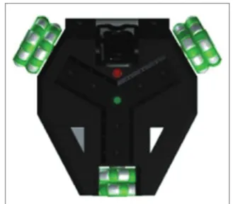
The experiments are implemented using the three omni-wheel robot. The omni-omni-wheel robot could move in any direction. Figure 4 shows the robot.
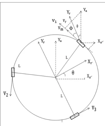
Kinematical equation can be obtained from its kine-matical diagram described in Figure 5.
In Figure 5, ½Xa YaT is the world coordinates,
Xr Yr
½ T represents a moving frame with respect to the center of the robot,uis the rotation angle which is positive in the counterclockwise direction, Lis the dis-tance between the robot and the center of each wheel, and½V1 V2 V3T stands for the translational velocity of each wheel.
After reasoning, Vi of each wheel can be obtained
and described in the vector–matrix form as follows
V1 V2 V3 2
4 3
5=Pð Þ u
_
Xa _
ya
_
u 2
4 3
5 ð23Þ
where
Pð Þu =
sinðu+308Þ cosðu+308Þ L
sinð308uÞ cosð308uÞ L
cosu sinu L
2
4
3
5 ð24Þ
Figure 4. Omni-wheel robot. Algorithm 2:Case adaptation.
num = number(retrieved case/cases); count = 1;
If(num.1)
shortest = Distance of the first retrieved case; Fori = 2 to num
IfDistance(i)\shortest shortest = Distance(i);
count = i; End End
Return case(i); Else
Return case(1); End
Ifshortest.5
Modify the turning direction according to the current case. End
In fact, the velocity of each wheel has been given in advance. We can obtain the orientation and speed of the robot through another equation transformed by equation (25)
_
Xa _
ya
_
u 2
4 3
5=P 1
u
ð Þ
V1 V2 V3 2
4 3
5 ð25Þ
where
P1ð Þu =
2
3sinðu+308Þ 2
3sinðu308Þ 2
3cosu 2
3cosðu+308Þ 2
3cosðu308Þ 2
3sinu 1
3L
1
3L
1
3L
2
6 6 6 6 6 4
3
7 7 7 7 7 5
ð26Þ
Simulation
Based on kinematical equation described above, three different obstacle cases which retrieved by the proposed two basic build-in case models have been designed to run the experiments, respectively, including one linear obstacle, one concave polygon obstacle, and one con-vex polygon obstacle. In order to test the performance of global planning, a complex scenario is also designed, which is composed of multi-obstacles.
To model the unknown environment in MATLAB (version: 2010a), the parameter is set as below. Size of
whole map is 50 cm3 50 cm, starting point coordinate is (220, 220), target point coordinate is (20, 20), and the velocity of the robot is 1 cm/s. There is no pause during the whole traveling process. Robot should arrive at the target point at a predetermined time; if not, the experiment result will be judged as failed. Each scenario was repeated 50 times to distinguish system with CBR from system without CBR. The distance and time below represent the average path length and average time consumption from start point to target point, respectively.
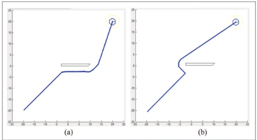
One linear obstacle. In scenario 1, the linear obstacle consists of four walls including four sides and four angles. Every side or angle is a separate case; in total, there are eight cases in this scenario. Planning path with EMMAPF method, robot will update its move direction on case base constantly by comparing dist1 withdist2 when it meets the obstacle wherever on the four sides or the four angles. At the same time, system calculates the corresponding transfer angle, and finally realizes the robot navigation and obstacle avoidance.
The specific implementation process is as follows. At first, in the first corner, the robot met an angle-type obstacle. After comparing the value betweendist1 and dist2, system judged that draw toward the vertical wall will be better. It can be known that rightAngle=0,
angle=p=2 (in Figure 6(b)), calculated by equation
(13), we got the result thatresetdirection=p=2, which
means that the robot will do a vertical movement. In this case, the robot executed a circular motion around the corner instead of the previous movement toward the corner. Second, in the second corner, after finishing circular motion, robot walked along the vertical wall. At last, in the third point, the intended direction of robot ran away from the corner, so that there is no need to make the robot to flee from the influence of obstacles. In this scenario, there is eight basic cases to be included in a one linear obstacle case.
As it can be seen from Table 1, ‘‘EMMAPF’’ method reduced the average time almost by 9.7%, and the dis-tance from start point to target point was reduced almost by 6.2%.
One convex polygon obstacle. In scenario 2, the convex polygon consists of four walls. Every side or angle is a Figure 5. Kinematical diagram of the omni-wheel robot.
Table 1. Average time and distance of the path in scenario 1.
Scenario 1 Time (s) Distance (cm)
MAPF 62.703 63.748
EMMAPF 54.578 59.616
separate case; in total, there are eight cases in this sce-nario. Planning path with EMMAPF method, robot will update its move direction on case base constantly by comparing dist1 with dist2 when it met a linear obstacle in the first corner. After comparing the value between dist1 and dist2, system judged that move toward upper left will be better. It can be known that
rightAngle=5p=6(in Figure 7(b)), calculated by
equa-tion (12), we got the result that resetdirection=5p=6,
which means that robot will move toward upper left. At the second corner, robot met an angle-type obstacle. Similarly, calculated by empirical formula, we got the result that robot will deflect toward upper right; deflec-tive angle will be the global perspecdeflec-tive of the border length that is equal to 6. On the sharp point robot invoked ‘‘driveCorner’’ function to make the path
smoother. Then, after the end of the arc movement, robot met a linear case to navigate it to the target along the wall. In the third corner, an angle-type obstacle case was used to make it flee from the influence of obstacle and move to the target directly. In this sce-nario, it consists of eight basic cases, but there are four basic cases to be used by EMMAPF method to achieve the best path planning.
As it can be seen from Table 2, ‘‘EMMAPF’’ method reduced the average time almost by 7.5%, and the dis-tance from start point to target point was reduced almost by 3.0%.
One concave polygon obstacle. There are many shapes of concave obstacles. In this scenario, we chose a common shape, which shows in Figure 8 to do this simulation. Figure 6. Path with (a) ‘‘MAPF’’ method and (b) ‘‘EMMAPF’’ method in scenario 1.
The concave polygon consists of eight walls including eight sides and eight angles. Besides the identical cases, there are total nine separate cases in this scenario. In this simulation, totally there are five used cases during robot’s movement including two linear cases and three angle-type cases. The path planning result of two linear walls with border length that is equal to 14 and 2 is horizontal movement to the right. For those three-angle-type cases where the lengths of left and right side are (2, 5), (2, 7), and (14, 5), the deflective angles are
7p=4, p=4, and7p=4, respectively. As it can be seen
from Figure 8, EMMAPF changed the path of MAPF and achieved better path navigation.
Scenario 3 is a concave polygon obstacle environ-ment. Using CBR method is more effective in the per-formance of time and distance. The data in Table 3 show that using this method reduced the traveling time by 3.3% and distance reduced by approximately 3.2%.
Complex multi-obstacles. In scenario 4, we built an overall case base consists of triangle, trapezium, parallelogram, and the other basic obstacles which were introduced in Figure 10. Through case retrieval system, we test the most similar matching case. If there is any unreason-able path, correct it and re-store into the case base. In addition, fuzzy logic method7is selected to be tested in
the contrast experiment. Fuzzy logic, similar to our proposed EMMAPF, is also a method to deal with path planning in unknown and dynamic environment in real time, and it could also achieve optimal local path planning.
For fuzzy logic method, the movement of the robot in the system is done by a fuzzy inference system (FIS) planner. The FIS takes four inputs. There are angle to goal (a), distance from goal (dg), distance from obstacle
(d0), and turn to avoid obstacle (t0). There is a single output that measures the angle (b) that the robot should turn along the direction. The rules can be classi-fied into two major categories. The first category of rules tries to drive the robot toward the goal. The sec-ond category of rules tries to save the robot from obstacles. If an obstacle is very near, the second cate-gory of rules becomes very dominant. A total of 11 rules are identified; these are given in Figure 9. The numbers in parentheses denote the weights.
The comparison of path performance is shown in Figure 10 and Table 4.
In Figure 10, it is obvious that robot gets trapped in the local minimum problem and cannot reach the target point using fuzzy logic method, while MAPF and EMMAPF method can complete robot autono-mous navigation effectively. The robot will unable to complete effective path navigation when it meets new Table 2. Average time and distance of the path in scenario 2.
Scenario 2 Time (s) Distance (cm)
MAPF 63.05 66.91
EMMAPF 58.29 64.56
MAPF: modified artificial potential field method; EMMAPF: experience mixing with modified artificial potential field method.
Figure 8. Path with (a) ‘‘MAPF’’ method and (b) ‘‘EMMAPF’’ method in scenario 3.
Table 3. Average time and distance of the path in scenario 3.
Scenario 3 Time (s) Distance (cm)
MAPF 59.34 62.07
EMMAPF 57.56 60.86
and unknown environment, because the rules of fuzzy logic are preset. However, the actual situation is that not all the rules can be considered in advance. In this article, as described in the previous section, the local minima problem can be solved using MAPF method. Moreover, it can also be solved by our proposed EMMAPF which is an optimal method to combine MAPF with CBR mechanism. In CBR, the cases of complex obstacles can be retrieved by two basic build-in case models which is composed of ‘‘lbuild-inear-type obstacle model’’ and ‘‘angle-type obstacle model.’’ In the process of the global obstacle avoidance, system will invoke CBR algorithm using its past experience to achieve obstacle avoidance when obstacles are recog-nized as known type; otherwise, it will invoke the ‘‘MAPF’’ method to solve the current problem, and the new case will be self-retained into the case base if the obstacle type is considered as an unknown. In addition, as can be seen from the data in Table 4, by comparing our proposed EMMAPF method with MAPF method, the runtime is reduced by approxi-mately 12.1%, and the distance is reduced by 7.8%; although the time-consuming performance of fuzzy
logic method is good and the path distance of local path is optimal in some cases, there exists some abnor-mal problems such as the path is not optiabnor-mal and the target is unable to be reached when the rules of fuzzy logic are incomplete.
Simulation result analysis
Based on the experimental results, we can conclude that the path of ‘‘EMMAPF’’ method is more optimal than ‘‘MAPF’’ method and ‘‘fuzzy logic’’ algorithm. The Figure 9. FIS rules.
Figure 10. Path with (a) ‘‘MAPF,’’ (b) ‘‘EMMAPF,’’ and (c) ‘‘Fuzzy logic’’ method in scenario 4.
Table 4. Average time and distance of the path in scenario 4.
Scenario 4 Time (s) Distance (cm)
MAPF 100.415 78.458
EMMAPF 88.260 72.312
Fuzzy logic 71.307 (uncompleted) 58.833 (uncompleted)
path generated through ‘‘MAPF’’ method is safe but long and passes through many unnecessary places. Using ‘‘EMMAPF’’ method to obtain the available prior experience can help the robot to make the best decisions when it encounters the obstacles.
Real test
In order to control the real-time movement of the robot to verify the effectiveness of this method, we take an actual test based on a Kinect sensor with the mobile robot.
Kinect is a motion sensing input device that is used by Microsoft Xbox 360video game console and WindowsPCs. Besides the main business as a gaming device, it is also treated as a good sensor to identify the category of obstacles for robot. In brief, Kinect includes a color (RGB) camera, an infrared depth sen-sor, an accelerometer, four microphones, and a motor to adjust the tilt. Its detection depth is up to 5 m.
Color camera obtains an actual image of the current environment. Infrared depth sensor collects the depth data, which indicates the distance between the objects and the camera. Regardless of the light condition around the environment, Kinect could capture 6403480 registered image and depth points at 30 frames/s. After analyzing the related environmental information, we could obtain the features of the obsta-cles. Figure 11 shows the process of the experiment. We implement our experiments based on the robot operating system (ROS) platform.
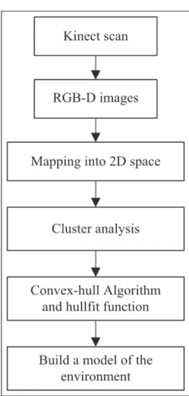
In fact, model environment depends on the sensor data type and the purpose of using generated map. Figure 12 shows how to build a model of the environment.21
Mapping into two-dimensional space. In the beginning, Kinect scans the environment to generate RGB-D images. Successive frames of RGB-D information are captured during the movements of the robot at 30 frames/s, and then obtain the point clouds from the depth image. A point cloud is always defined as a set of irregular, unorganized points in three dimensions (3D). point cloud data (PCD) files contain the message
including each point coordinate (x, y, and z) and the color information. Figure 13 illustrates an example of generating point cloud in our real-world test scene.
Because of the point cloud data are based on Kinect-centered coordinate, so we need to transform the points into world coordinates when we map the point cloud into a two-dimensional (2D) continuous space. Two steps have been taken. First, keep the points between the min and max height which Kinect could detect by equation (27). Second, map those point clouds into equivalent 2D continuous space by equation (28). (X,Y) is the corresponding coordinate that (x, y, andz) is mapped on
P=fðx,y,zÞjhmin\y\hmaxg ð27Þ
X,Y
ð Þ=ðuðzsinu+xcosuÞ,
v+ðzcosuxsinuÞÞ ð28Þ
Figure 11. The process of the experiment.
Kinect scan
RGB-D images
Cluster analysis Mapping into 2D space
Convex-hull Algorithm and hullfit function
Build a model of the environment
where (u,v) represents the coordinate of the Kinect and umeans the global angle of the Kinect.
Figure 14 shows the effect of mapping point cloud in Figure 13 (b) into 2D space.
The more the frames are captured, the more points are included in the 2D-mapped space. The 2D-mapped points with new frames would be added into the world coordinate with the increase in time.
Data clustering. The next step is to cluster the points of 2D map; some kinds of clustering algorithm have been
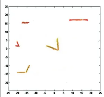
tried to apply in data clustering; in this research, density-based spatial clustering of applications with noise (DBSCAN) is the best approach which is capable of finding arbitrarily shaped clusters. It is very flexible with unusual shape of dense point areas. Figure 15 illustrates the resulting clusters which could represent one shape in the space.
Concave-hull approach. P Wasmeier22 implemented a function in MATLAB called hullfit, which could calcu-late a concave-hull of a data set. Two parts are included in this algorithm.
First, apply the concave-hull to obtain vertices of corresponding convex-hull and classify them as clock-wise. Next, calculate the distances among each two neighbors’ vertices to find any distance greater than maximum allowed distance. If any points returned, use some conditions to find another proper point in the data set as the next vertex.
More detailed description is introduced in Mojtahedzadeh.23 Here, we apply the function hullfit to represent obstacles with the best polygons to fit. Figure 16 shows one final model of the environment during the robot moving to the target.
Thus, we could get the category of the obstacle’s front shape by the Kinect sensor, such as line or con-cave polygon, which is the useful information of the obstacles used to complete the path planning. We imi-tate scenario 4 to verify the efficiency of ‘‘EMMAPF’’ algorithm in real world. The size of the area is 5 m3 5 m. Kinect is placed in the front of the omni-wheel robot.
The black dot in the top right corner of the scene is the target. We set the origin velocity of the robot at 0.1 m/s. Figure 17 shows the actual process of robot Figure 13. An example of generating point cloud. (a) RGB
image (left) and depth information (right) taken by a RGB-D camera and (b) point cloud.
Figure 14. Map point cloud into 2D space.
navigation in a complex multi-obstacle environment. The information of the obstacles is unknown in advance.
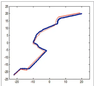
Table 5 illustrates the statistical data of experiments in simulation and actual test. Time used in actual test is a little more than in simulation, while distance is shorter. This deviation is caused by the fiction that exists between the wheels of robot and the floor.
As it can be seen from Figure 18, two paths are shown in different colors. Blue line represents the path in simulation environment, while the red line represents the actual path in real-time physical test environment. Except for the robot traveling around the corner, the deviation of the path is small. Figure 19 records that the path deviation exists on each moment in the move-ment. In fact, the deviation is small (\0.1 m) and is
acceptable. So, we can conclude that the ‘‘EMMAPF’’ algorithm could be applied in the real world successfully.
Conclusion and future work
In this article, a new approach EMMAPF which com-bines case-base reasoning method with the modified APF method is put forth to get an optimal path and Figure 16. The final model of the environment.
Figure 17. Process of the robot using ‘‘EMMAPF’’ method in a complex multi-obstacle environment.
Table 5. Comparison between simulation and actual test.
Scene area No. of
obstacles
Running time
Distance
Simulation 0.5 m30.5 m 6 88.26 s 0.723 m
Actual test 5 m35 m 90.13 s 7.024 m
Ratio 1:10 1:1 1:1.02 1:11.2
better algorithm efficiency. In CBR, we innovatively consider that all the complex obstacles are retrieved by two kinds of basic build-in obstacle models (linear obstacle and angle-type obstacle). In the process of the global obstacle avoidance, system will invoke CBR algorithm using its past experience to achieve obstacle avoidance when obstacles are recognized as known type; otherwise, it will invoke the ‘‘MAPF’’ method to solve the current problem, and the new case will be retained into the case base if the obstacle type is consid-ered as an unknown. In simulations, three different obstacle cases which retrieved by the proposed two basic build-in case models have been designed to run the experiments, respectively, including one linear obstacle, one concave polygon obstacle, and one con-vex polygon obstacle. In order to test the performance of global planning, a complex scenario is also designed, which is composed of multi-obstacles. We illustrated the obstacle avoidance process and effect of those four obstacle cases using our proposed EMMAPF com-pared with MAPF and fuzzy logic algorithm. In actual test, by acquiring the RGB-D images from the Kinect sensor and building the model of the final environment, robot could obtain the useful information of the obsta-cles and utilize the ‘‘EMMAPF’’ method to deal with path planning in unknown and dynamic environment in real time. According to simulation and actual test, we can come to the conclusion that this method has been proved applicable to the dynamic real-time obsta-cle avoidance under unknown and unstructured envi-ronment, and it greatly improved the performance of robot path planning that not only reduced the time consumption but also shorten the moving distance.
In future, there are two major issues that we need to pay more attention. One is to improve the performance of CBR in real time, some measures need be taken to shorten the time in searching and matching; otherwise,
time delay in CBR mechanism would lead to the failure of the obstacle avoidance. The other issue is to improve the accuracy of building a model of the environment. More different methods should be studied and com-pared in data clustering. The detection of the obstacles in the environment has a significant effect on the results of the ‘‘EMMAPF’’ method. With the development of this method, our system will become a true real-time system to deal with path planning for mobile robot in the future.
Acknowledgements
This article is a revised and expanded version of a paper enti-tled ‘‘Experience Mixed the Modified Artificial Potential Field Method’’ which presented at the IEEE/RSJ International Conference on Intelligent Robots and Systems (IROS 2013), held at Tokyo, Japan, during 3–8 November 2013.
Declaration of conflicting interests
The author(s) declared no potential conflicts of interest with respect to the research, authorship, and/or publication of this article.
Funding
The author(s) disclosed receipt of the following financial sup-port for the research, authorship, and/or publication of this article: This work was supported by the National Natural Science Foundation of China (Grant No. 61175094).
References
1. Khatib O. Real-time obstacle avoidance for manipula-tors and mobile robots.Int J Robot Res1986; 5: 90–98. 2. Lee MC and Park MG. Artificial potential field based
path planning for mobile robots using a virtual obstacle concept. In:Proceedings of the 2003 IEEE/ASME inter-national conference on advanced intelligent mechatronics, Kobe, Japan, 20–24 July 2003, vol. 2, pp.735–740. New York: IEEE.
3. Charifa S and Bikdash M. Adaptive boundary-following algorithm guided by artificial potential field for robot navigation. In: Proceedings of the IEEE workshop on robotic intelligence in informationally structured space, Nashville, TN, 30 March–2 April 2009, pp.38–45. New York: IEEE.
4. Li Q, Wang LJ, Chen B, et al. An improved artificial potential field method with parameters optimization based on genetic algorithms.J Univ Sci Technol B2011; 34: 202–206.
5. Guan-chen L, Jian-qiao Y and Si-yu Z. Artificial poten-tial field based receding horizon control for path plan-ning. In: Proceedings of the 24th Chinese control and decision conference (CCDC 2012), Taiyuan, China, 23– 25 May 2012, pp.3665–3669. New York: IEEE.
6. Song Q and Liu L. Mobile robot path planning based on dynamic fuzzy artificial potential field method. Int J Hybrid Inform Technol2012; 5: 85–93.
7. Kala R, Shukla A and Tiwari R. Fusion of probabilistic A* algorithm and fuzzy inference system for robotic path planning.Artif Intell Rev2010; 33: 307–327.
8. Qu H, Yang SX, Willms AR, et al. Real-time robot path planning based on a modified pulse-coupled neural
net-work model. IEEE T Neural Networ 2009; 20:
1724–1739.
9. Chen W and Qin H. Path planning of mobile robot based on hybrid cascaded genetic algorithm. In: Proceed-ings of the 9th world congress on intelligent control and automation, Taipei, Taiwan, 21–25 June 2011, pp. 501–504. New York: IEEE.
10. Pal SK and Shiu SCK.Foundations of soft case-based rea-soning. Hoboken, NJ: John Wiley & Sons, 2004.
11. Kruusmaa M. Global navigation in dynamic environ-ments using case-based reasoning.Auton Robot2003; 14: 71–91.
12. Urdiales C, Perez EJ, Va´zquez-Salceda J, et al. A purely reactive navigation scheme for dynamic environments using case-based reasoning.Auton Robot2006; 21: 65–78. 13. Hoda´l J and Dvorˇa´k J. Using case-based reasoning for mobile robot path planning. Eng Mech 2008; 15: 181–191.
14. Wang S and Min H. Experience mixed the modified arti-ficial potential field method. In:Proceedings of the IEEE/ RSJ international conference on intelligent robots and sys-tems, Tokyo, Japan, 3–7 November 2013. New York: IEEE.
15. Liu C, Cheng Y and Liu C. Anti-collision path planning for mobile robot based on modified potential field
method, http://en.cnki.com.cn/Article_en/CJFDTOTAL-DNDX2009S1024.htm
16. Lei L. Formation and coordinated control of multiple mobile robots. Wuhan, China: Huazhong University of Science and Technology, 2009.
17. Ge SS and Cui YJ. Dynamic motion planning for mobile robots using potential field method.Auton Robot 2002; 13: 207–222.
18. Wu XH and Zhou JJ. Kernel-based fuzzy k-nearest neighbor algorithm. In: Proceedings of the international conference on computational intelligent for modeling, con-trol and automat, Vienna, 28–30 November 2005, vol. 2, pp.28–30. New York: IEEE.
19. Chang PC, Lin JJ and Dzan WY. Forecasting of manu-facturing cost in mobile phone products by case-based reasoning and artificial neural network models. J Intell Manuf2012; 23: 517–531.
20. Shin K and Han I. A case-based approach using inductive indexing for corporate bond rating. Decis Support Syst 2001; 32: 41–52.
21. Henry P, Krainin M, Herbst E, et al. RGB-D mapping: using Kinect-style depth cameras for dense 3D modeling of indoor environments. Int J Robot Res 2012; 31: 647–663.
22. Wasmeier P. hullfit, http://www.mathworks.com/matlab central/fileexchange/6243-hullfit (accessed 2 November 2015).