J. Braz. Soc. Mech. Sci. & Eng. vol.32 número4

(1)

Viscosity Behavior of Mixtures of CO

2

and Lubricant Oil

Moisés A. Marcelino Neto

moises@polo.ufsc.br

Experimental data on the viscosity of mixtures of CO2 and lubricant oil were acquired and Federal University of Santa Catarina

correlated using an excess-property approach based on the classical Eyring liquid Department of Mechanical Engineering

viscosity model. Three oils of different types and viscosity grades (alkylbenzene AB ISO 88040-900 Florianópolis, SC, Brazil _{32, mineral MO ISO 50 and polyol ester POE ISO 68) were evaluated at temperatures} ranging from 36.5 to 82°C. The excess activation energy for viscous flow was successfully correlated as a function of temperature and concentration using Redlich-Kister polynomial

Jader R. Barbosa, Jr.

expansions with up to three terms. Large departures from the ideal solution viscosity behavior have been identified in all mixtures. The nature of the observed deviations has jrb@polo.ufsc.br

been explored in the light of their dependence on temperature, refrigerant concentration Federal University of Santa Catarina

and oil type. The Katti and Chaudry (1964) model of the activation energy of viscous flow Department of Mechanical Engineering

displayed the best correlation of the experimental data, with RMS deviations of 4.6% (AB 88040-900 Florianópolis, SC, Brazil _{ISO 32), 3.3% (MO ISO 50) and 2.8% (POE ISO 68).}

Keywords: CO2-lubricant oil mixture, viscosity, experimental data, modeling

using an excess-property approach based on the classical Eyring liquid viscosity model. The Eyring theory correlations of Grunberg and Nissan (1949), Katti and Chaudry (1964) and McAllister (1960) have been utilized. The best agreement between model and experimental data was obtained with the Katti and Chaudry (1964) equation.

Introduction

1

There are several refrigeration applications where CO2 (R-744) is well suited as a primary refrigerant (Pettersen, 1999). Due to its unique characteristics, such as chemical stability, toxicity, non-flammability, low-cost, low GWP (Global Warming Potential) and zero ODP (Ozone Depletion Potential), the use of CO2 in some specific applications appears especially promising in a global

scenario where more stringent environmental legislation is applied.

_Nomenclature

As far as CO2 refrigeration systems are concerned, the

compressor design requires special attention due to the inherently lower system performance encountered in the CO2 trans-critical cycle when compared with the standard sub-critical cycle usually associated with other refrigerants (Gosney, 1982). In this context, a crucial aspect of the CO2 compressor design is related to the performance and reliability of the bearings system. It is of utmost importance that the variation of the physical properties of the lubricant mixture with respect to temperature and refrigerant concentration are taken into account during all stages of the system design. Despite the increasing number of publications dealing with the determination of physical properties of mixtures of CO2 and lubricant oils and some of their precursors (Yokozeki, 2007; Bobbo et al., 2007; Pensado et al., 2008), more research is still needed before the most suitable lubricants, with specific lubrication characteristics for a variety of CO2 refrigeration applications, are finally selected.

= Activation energy for viscous flow, J/kmol +

i

G +

E

G = Excess activation energy for viscous flow, J/kmol h = Planck’s constant [6.626 x 10-34], Js

M = Molar mass, kg/kmol

Na = Avogrado’s number [6.023 x 1026], kmol-1 P = Pressure, MPa

R = Universal gas constant [8.314], kJ/kmol.K T = Temperature, K or °C

V = Molar volume, m3/kmol Vi = Molar volume of component i, m

3 /kmol wi = Mass fraction of component i, kg/kg xi = Mole fraction of component i, kmol/kmol

Greek Symbols

η = Dynamic viscosity, cP or mPa.s ν = Kinematic viscosity, m2/s Recent appraisals of the experimental and theoretical work on

the determination of the physical properties of mixtures of CO2 and lubricant oil have been presented by Seeton and Hrnjak (2006), Bobbo et al. (2006), Marcelino Neto and Barbosa (2007) and Yokozeki (2007). Undoubtedly, in the open literature, the most extensively studied mixtures of CO2 and oil are those involving polyol esters (POE) and polyalkylene glycols (PAG). Significantly less work has been devoted to characterizing mixtures of CO2 and other oil types, such as mineral (MO), polyalphaolefin (PAO) and alkylbenzene (AB). Moreover, the number of works in which the viscosity behavior of CO2-lubricant mixtures is investigated in detail is still rather limited.

ρ = Mass density, kg/m3

Experimental Work

Experimental Apparatus and Procedure

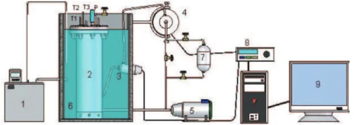
The experimental facility is schematically illustrated in Fig. 1 (Marcelino Neto and Barbosa, 2007, 2009). A specified amount of lubricant oil is placed in the 4 L equilibrium cell (2). A vacuum of 0.04 mbar is generated in the apparatus to remove moisture and dissolved gases. An initial amount of refrigerant is fed into the cell. The system temperature is set by a thermostatic bath (1) that circulates service water through a tank (6) in which the equilibrium cell is fully immersed. In the present experiments, the pressure of the oil-refrigerant mixture is, therefore, the dependent variable. The equilibrium cell is instrumented for absolute pressure, P, and the temperature of the fluids in the cell is recorded by three type-T thermocouples (T1, T2, T3) located at three distinct heights to The objective of this paper is to present experimental data on the

liquid viscosity of mixtures of CO2 and three lubricants, namely, a POE ISO 68, a MO ISO 50 and an AB ISO 32. The data points were obtained at pressures between 0.9 and 5.7 MPa and temperatures between 36.5 and 82°C. The liquid mixture viscosity was correlated

(2)

pump (5) moves the liquid oil-refrigerant mixture through the experimental facility. The speed of the electrical motor is set at its minimum value (12 Hz). The mixture first flows through a Coriolis-type mass flow transducer (4) that records flow rate, temperature and liquid density. Then, an oscillating piston viscometer (3) registers temperature and dynamic viscosity of the liquid mixture. The solubility of the mixture is measured gravimetrically using a liquid mixture sample collected in a 150 mL cylinder (7). The experimental apparatus is integrated with a signal conditioning module (8) and a computerized system for data acquisition and treatment (9). The tank (top, sides and bottom), connection tubing and instrumentation (Coriolis flow meter, pump and sampling cylinder) are thermally insulated to prevent heat loss. The temperature variation between the viscometer, the mass flow/density meter and test cell was within the uncertainty level set during the calibration of the thermocouples. The experimental procedure for obtaining the mixture solubility has been outlined in Marcelino Neto and Barbosa (2007, 2009).

Viscosity Modeling

Liquid Viscosity Models

The Eyring theory (Glasstone et al., 1941) for the viscosity of pure liquids can be extended for binary mixtures as follows (Oswal and Desai, 2001):

⎟ ⎟ ⎠ ⎞ ⎜

⎜ ⎝

⎛ + ₊ + ₊ +

=

RT E G G x G x h a N

ηV exp 1 1 2 2 (1)

or in a more suitable form:

( )

(

)

(

)

RT E G V x V x V

+ + +

= ₁ln ₁₁ ₂ln ₂ ₂

lnη η η (2)

where η is the mixture dynamic viscosity, ηi is the dynamic viscosity of component i, V is the mixture molar volume, Vi is the molar volume of component i, Na is the Avogadro constant, h the Planck constant, R is the universal gas constant, T is the absolute temperature, xi is the mole fraction of component i, Gi+ is the activation energy for viscous flow of component i and GE+ is the excess activation energy for viscous flow. Subscripts 1 and 2 stand for the refrigerant and lubricant oil, respectively.

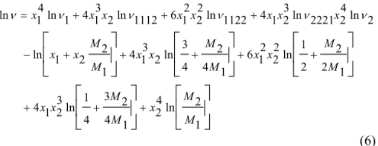
Katti and Chaudry (1964) modeled the activation energy for viscous flow in Eq. (2) using a polynomial Redlich-Kister type expansion given by

Figure 1. Schematic representation of the experimental rig.

The temperature measurement uncertainty was estimated at ±0.2°C (68% confidence level). The uncertainty of the density measurements (estimated from the manufacturer specifications) was ±1% of the absolute reading (95% confidence level). The uncertainty of the viscosity measurements (estimated from the manufacturer specifications) was ±1% of the full scale (68% confidence level). It should be observed that, because of interchangeable pistons, the uncertainty is ±0.1 cP for the 0.1-10 cP piston, and ±1 cP for the 1-100 cP piston. The uncertainty of the pressure transducer (estimated from the manufacturer specifications) was ±0.15% FS (0.3 bar) and that of the balance was ±0.3 g. After an error propagation analysis (Marcelino Neto, 2006), the uncertainty in the solubility measurement was determined at ±0.5 g/kg. The experimental procedure was validated with vapor pressure and density measurements of pure CO2 and with density and viscosity of an ISO 10 lubricant oil, whose properties have been made available from its manufacturer (Marcelino Neto and Barbosa, 2007).

L + − − + − − + = +

RT x x x D

RT x x D

RT E

G ₀₁ ₂ ₁(2 ₁ 1)(₁ ₁2) ₂(2₁ 1)2( ₁ ₁2) ₍₃₎

where Di are constants with i = 0,1,2,...N. In the present work, the Katti and Chaudry expansion was truncated in the third term.

The Grunberg and Nissan (1949) model assumes an ideal solution behavior (V = x1V1 + x2V2) in which the mixture viscosity is correlated from

( )

L + − − +

+ − − + + +

=

) 2 1 1 ( 2 ) 1 1 2 ( 2

) 2 1 1 )( 1 1 2 ( 1 2 1 0 2 ln 2 1 ln 1 ln

x x x G

x x x G x x G x

x η η

η

(4)

In the present paper, the Grunberg and Nissan correlation has been employed in two different ways. In the first approach, henceforth referred to as the G-N approach, G0 is correlated as a linear function of the CO2 mole fraction for each temperature (Tomida et al., 2007):

Experimental Conditions

(5)

( )

₁

( )

₁

0

0 T T x

G =Γ +Γ

The experimental conditions of the present experiments are as follows. Solubility, liquid density and viscosity of CO2/MO ISO 50, CO2/AB ISO 32 and CO2/POE ISO 68 oil mixtures were measured at temperatures between 36.5 and 82°C. CO2 was supplied by AGA (99.9% pure) and the lubricants were supplied by Embraco. The molar masses of the lubricants are 355 kg/kmol (MO), 375 kg/kmol (AB) and 763 kg/kmol (POE). The molecular structures of the lubricants have not been disclosed to the present authors as they represent proprietary information.

and the remaining coefficients Gi are assumed equal to zero. In the second approach, the G-N2 approach, the series are truncated in the third term and the coefficients G0, G1 and G2 are assumed independent of temperature and are determined from a best-fit to the experimental data.

(3)

⎥

⎦

⎤

⎢

⎣

⎡

⎥

⎦

⎤

⎢

⎣

⎡

⎥

⎦

⎤

⎢

⎣

⎡

⎥

⎦

⎤

⎢

⎣

⎡

⎥

⎦

⎤

⎢

⎣

⎡

+ + + + + + + + − + + + = 1 2 ln 4 2 1 4 2 3 4 1 ln 3 2 1 4 1 2 2 2 1 ln 2 2 2 1 6 1 4 2 4 3 ln 2 3 1 4 1 2 2 1 ln 2 ln 4 2 2221 ln 3 2 1 4 1122 ln 2 2 2 1 6 1112 ln 2 3 1 4 1 ln 4 1 ln M M x M M x x M M x x M M x x M M x x x x x x x x x

x ν ν ν ν ν

ν

(6)

where ν is the kinematic viscosity of mixture, νi is the kinetic viscosity of pure component i at the same temperature and pressure as the mixture, and Mi is the molar mass. ν1112, ν1122, ν2221 are fitting coefficients calculated from a best-fit to the experimental data.

Implementation

The models were implemented in the Engineering Equation Solver – EES (Klein, 2007), and the genetic algorithm routines available in EES were employed in the determination of the models’ coefficients. The physical properties of pure CO2 were obtained from EES and the properties of the pure lubricants (density and viscosity) were derived from polynomial fittings to our own experimental data. To evaluate the prediction ability of the correlations, the following quantities can be defined

(

)

∑ = − = n i _i i i cal

n 1 2_exp,

2 exp, , 100 RMS η η η (7) ∑ = − = n i i i i cal n 1 exp, exp, , 100 AAD η η η (8) ∑ = − = n i i i i cal n 1 exp, exp, , 100 Bias η η η (9)

where, in the McAllister (1960) model, η is substituted by ν in the above equations.

Results and Discussion

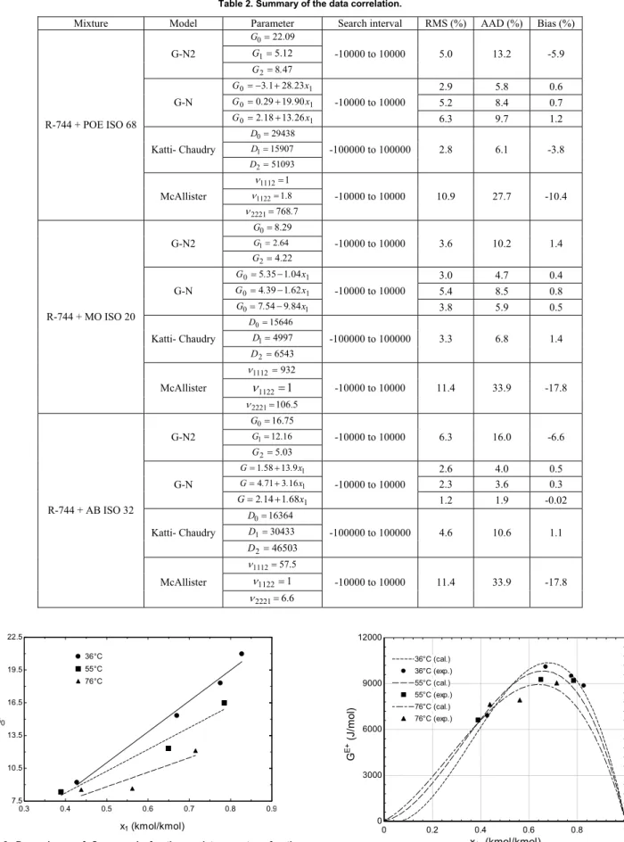
The experimental data for the mixture viscosity, density and molar solubility are presented in Table 1 as a function of pressure and temperature. The model predictions are summarized in Table 2, where the search intervals employed in the calculation of the fitting parameters are also presented.

A direct comparison between the G-N2 model and the Katti and Chaudry (1964) correlation (both with a three-term expansion of the activation energy parameter) indicates that the latter has predicted

the data with a better agreement. Although there may be several reasons for this particular result, perhaps the most apparent explanation seems to be the fact that the severe non-ideality of the mixture molar volume is not considered in the Grunberg and Nissan (1949) model. The McAllister (1960) model does not perform well under the conditions evaluated in the present work.

Contrary to what has been observed for the CO2/MN ISO 50 and CO2/AB ISO 32 mixtures, the performance of Grunberg and Nissan (1949) for the CO2/POE ISO 68 mixture does not necessarily improve when the temperature dependence approach of Tomida et al. (2007) is adopted. In Table 2, the correlations for G0 as a function of temperature are presented as a function of increasing temperature from top to bottom and Figures 2 to 4 present the dependence of G0 on temperature and composition and the variations of GE+(the activation energy of Katti and Chaudry) and of G (the three term expansion on the right hand side of the Grunberg and Nissan model – Eq. 4) as a function of temperature and composition for the CO2/POE ISO 68 mixture. Positive deviations are observed at all temperatures, which characterize stronger interactions between molecules of different species (Grunberg and Nissan, 1949).

Table 1. Experimental data.

T(°C) P(MPa) x1 (kmol/kmol) ρ (kg/m³)

Mixture η (cP)

0.9 0.4275 965.3 26.6

2.2 0.6692 967.5 12.8

4.1 0.7755 968.7 4.6

36.5

5.2 0.8274 968.8 2.5

1.1 0.4381 952.7 16.6

3.4 0.5619 952.3 6.6

R-744 + POE 55.5

5.8 0.7150 950.6 2.7

ISO 68

1.1 0.3890 938.7 9.5

3.4 0.6493 938.0 4.8

76.5

5.7 0.7846 930.4 2.7

1.0 0.2070 911.6 27.0

3.4 0.3653 914.9 9.9

40.5

5.5 0.5085 917.6 4.3

1.2 0.1417 902.0 11.3

3.4 0.3540 904.2 5.9

R-744 + MO 59.7

5.6 0.4237 905.0 2.7

ISO 50

1.2 0.1520 898.1 5.6

3.8 0.2946 892.9 2.8

81.5

5.5 0.4044 895.9 1.9

1.4 0.2512 873.1 19.9

3.6 0.5173 861.4 8.7

40.5

5.1 0.6681 869.7 4.3

1.3 0.1942 864.2 12.4

3.5 0.4053 856.8 5.5

R-744 + AB 57.7

5.4 0.5286 866.6 3.6

ISO 32

1.4 0.2115 859.1 7.0

3.5 0.3611 859.1 3.8

69.2

(4)

Table 2. Summary of the data correlation.

Mixture Model Parameter Search interval RMS (%) AAD (%) Bias (%)

22.09

0=

G 5.12

1=

G

G-N2 -10000 to 10000 5.0 13.2 -5.9

47 8

2 .

G =

1 0 3.1 28.23x

G =− + 2.9 5.8 0.6

1 0 0.29 19.90x

G = + 5.2 8.4 0.7

G-N -10000 to 10000

1 0 2.18 13.26x

G = + 6.3 9.7 1.2

29438

0= D R-744 + POE ISO 68

15907

1=

D -100000 to 100000 2.8 6.1 -3.8

Katti- Chaudry

51093

2= D

1

1112=

ν

1.8

1122=

ν -10000 to 10000 10.9 27.7 -10.4

McAllister

7 768

2221= .

ν 8.29

0=

G

2.64

1=

G -10000 to 10000 3.6 10.2 1.4

G-N2

4.22

2=

G

1 0 5.35 1.04x

G = − 3.0 4.7 0.4

1 0 4.39 1.62x

G = − 5.4 8.5 0.8

G-N -10000 to 10000

1 0 7.54 9.84x

G = − 3.8 5.9 0.5

15646

0= D R-744 + MO ISO 20

4997

1=

D -100000 to 100000 3.3 6.8 1.4

Katti- Chaudry

6543

2=

D 932

1112=

ν

1 1122=

ν -10000 to 10000 11.4 33.9 -17.8

McAllister

106.5

2221=

ν 16.75

0=

G

12.16

1=

G -10000 to 10000 6.3 16.0 -6.6

G-N2

5.03

2=

G

1

9 13 58 1. . x

G= + 2.6 4.0 0.5

1

16 3 71 4. . x

G= + -10000 to 10000 2.3 3.6 0.3

G-N

1

68 1 14

2. . x

G= + 1.2 1.9 -0.02

16364

0=

D

R-744 + AB ISO 32

30433

1=

D

Katti- Chaudry -100000 to 100000 4.6 10.6 1.1

46503

2=

D 57.5

1112=

ν

1 1122=

ν -10000 to 10000 11.4 33.9 -17.8 McAllister

6.6

2221= ν

0 0.2 0.4 0.6 0.8 1

0 3000 6000 9000 12000

x1 (kmol/kmol)

G

E+

(J

/m

o

l)

36°C (cal.) 36°C (cal.)

55°C (cal.) 55°C (cal.)

76°C (cal.) 76°C (cal.) 36°C (exp.) 36°C (exp.)

55°C (exp.) 55°C (exp.)

76°C (exp.) 76°C (exp.)

0.3 0.4 0.5 0.6 0.7 0.8 0.9

7.5 10.5 13.5 16.5 19.5 22.5

x1 (kmol/kmol)

G0

36°C 36°C

55°C 55°C

76°C 76°C

Figure 2. Dependence of G0 on mole fraction and temperature for the

CO2/POE ISO 68 mixture. _{Figure 3. Correlation of the activation energy of Katti and Chaudry (1964)}

(5)

Figures 7 to 9 present comparisons between the Katti and Chaudry (1964) correlation and the G-N approach for the three mixtures. Despite the better agreement of the latter model for the CO2/MO ISO 50 and CO2/AB ISO 32 mixtures, the Katti and Chaudry (1964) model is recommended for all three mixtures, because it is easier to apply at intermediate temperatures that have not been correlated during the experiments.

0 0.2 0.4 0.6 0.8 1

0 1 2 3 4

x1 (kmol/kmol) G

36°C (cal.) 36°C (cal.)

55°C (cal.) 55°C (cal.)

76°C (cal.) 76°C (cal.) 36°C (exp.) 36°C (exp.)

55°C (exp.) 55°C (exp.)

76°C (exp.) 76°C (exp.)

0 0.2 0.4 0.6 0.8 1

10-2

10-1

100

101

102

x1 (kmol/kmol)

η (cP)

36o_{C (exp.)}

55o_{C (exp.)}

76o_{C (exp.)}

36oC (G-N)

55o_{C (G-N)}

76o_{C (G-N)}

36o_{C (exp.)}

55o_{C (exp.)}

76o_{C (exp.)}

36o_{C (exp.)}

55o_{C (exp.)}

76o_{C (exp.)}

36o_{C (exp.)}

55o_{C (exp.)}

76o_{C (exp.)}

36o_{C (exp.)}

55o_{C (exp.)}

76o_{C (exp.)}

36o_{C (exp.)}

55o_{C (exp.)}

76o_{C (exp.)}

36o_{C (exp.)}

55o_{C (exp.)}

76o_{C (exp.)}

36o_{C (exp.)}

55o_{C (exp.)}

76o_{C (exp.)}

36o_{C (exp.)}

55o_{C (exp.)}

76o_{C (exp.)}

36o_{C (exp.)}

55o_{C (exp.)}

76o_{C (exp.)}

36o_{C (exp.)}

55o_{C (exp.)}

76o_{C (exp.)}

36o_{C (exp.)}

55o_{C (exp.)}

76o_{C (exp.)}

36o_{C (exp.)}

55o_{C (exp.)}

76o_{C (exp.)}

36oC (K-C)

55o_{C (K-C)}

76o_{C (K-C)}

R-744 + POE ISO 68

Figure 4. Correlation of the non-ideal three term expansion parameter of the Grunberg and Nissan (1949) correlation (CO2/POE ISO 68 mixture).

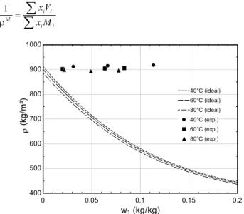
The mass density of CO2/MO ISO 50 and CO2/AB ISO 32 as a function of temperature is presented in Figs. 5 and 6, where a significant departure from the ideal mixture behavior (calculated from Eq. 10) is clearly observed.

Figure 7. Viscosity of the CO2/POE ISO 68 mixture and comparison with

the Katti and Chaudry (1964) and G-N models.

∑

=

ρ i i

i i id

M x

V x

1 (10)

0 0.2 0.4 0.6 0.8 1

10-2 10-1

100

101

102

x1 (kmol/kmol)

η (cP)

40o_{C (exp.)}

60o_{C (exp.)}

80o_{C (exp.)}

40o_{C (G-N)}

60o_{C (G-N)}

80o_{C (G-N)}

40o_{C (K-C)}

60o_{C (K-C)}

80o_{C (K-C)}

R-744 + M O ISO 50

0 0.05 0.1 0.15 0.2

400 500 600 700 800 900 1000

w1 (kg/kg)

ρ

(k

g

/m

³)

40°C (ideal) 40°C (ideal)

40°C (exp.) 40°C (exp.)

60°C (exp.) 60°C (exp.)

80°C (exp.) 80°C (exp.)

Figure 8. Viscosity of the CO2/MO ISO 50 mixture and comparison with the

Katti and Chaudry (1964) and G-N models (Grunberg and Nissan, 1949). Figure 5. Experimental liquid mass density of the CO2/MO ISO 50 mixture.

0 0.05 0.1 0.15 0.2

400 500 600 700 800 900 1000

w1 (kg/kg)

ρ

(k

g/

m

³)

40°C (exp.) 40°C (exp.) 57°C (ideal) 57°C (ideal)

57°C (exp.) 57°C (exp.)

70°C (exp.) 70°C (exp.)

0 0.2 0.4 0.6 0.8 1

10-2

10-1

100 101

102

x1 (kmol/kmol)

η (cP)

40oC (exp.)

57oC (exp.)

67oC (exp.)

40o_{C (G-N)}

57o_{C (G-N)}

67oC (G-N)

40o_{C (K-C)}

57o_{C (K-C)}

67oC (K-C)

R-744 + AB ISO 32

Figure 6. Experimental liquid mass density of the CO2/AB ISO 32 mixture. _{Figure 9. Viscosity of the CO}₂_{/AB ISO 32 mixture and comparison with the}

(6)

Glasstone, S., Laidler, K.J., Eyring, H., 1941, “The Theory of Rate Processes”, McGraw-Hill, NY.

Conclusions

Gosney, W.B., 1982, “Principles of Refrigeration”, Cambridge University Press, New York.

The present paper put forward new data on the viscosity of a mixture of CO2 (R-744) and three lubricant oils (POE ISO 68, MO ISO 50 and AB ISO 32). An experimental facility that enables the simultaneous measurement of the viscosity, density and solubility has been utilized. The data were obtained at three different temperatures in the range of 36.5 and 82°C. The viscosity data have been correlated with the Grunberg and Nissan (1949), Katti and Chaudry (1964) and McAllister (1960) correlations. When a three-term polynomial expansion of the excess activation energy with temperature independent coefficients is employed in the Grunberg and Nissan (1949) and Katti and Chaudry (1964) models, the latter presents a better correlation of the experimental data. Contrary to what has been observed for the MN ISO 50 and AB ISO 32 mixtures, using the Grunberg and Nissan (1949) approach with temperature dependent coefficients does not improve the prediction for the POE ISO 68 mixture. The performance of the McAllister (1960) correlation has been less satisfactory than those of the other models.

Grunberg, L., Nissan, A.H., 1949, “Mixture law for viscosity”, Nature, Vol. 164, pp. 799-800.

Katti, P.K., Chaudry, M.M., 1964, “Viscosities of binary mixtures of benzil acetate with dioxane, aniline and m-cresol”, Journal of Chemical, Vol. 9, pp. 442-443.

Klein, S.A., 2007, Engineering Equation Solver, F-Chart Software. Marcelino Neto, M.A., 2006, “Characterization of thermophysical properties of mixtures of lubricant oil and natural refrigerants” (in Portuguese), MEng dissertation, Federal University of Santa Catarina, Florianópolis, SC, Brazil.

Marcelino Neto, M.A., Barbosa Jr., J.R., 2007, “Solubility and Density of Mixtures of R-744 and Two Synthetic Lubricant Oils”, Proceedings of the 22nd International Congress of Refrigeration, Beijing, China, Paper ICR07-B1-1133, August 21-26.

Marcelino Neto, M. A., Barbosa Jr., J. R., 2009, “Phase and volumetric behaviour of mixtures of carbon dioxide (R-744) and synthetic lubricant oils”, The Journal of Supercritical Fluids, Vol. 50, pp. 6-12.

McAllister, R.A., 1960, “The viscosity of liquid mixtures”, AIChe Journal, Vol. 6, pp. 427-430.

Oswal, S.L., Desai, H.S., 2001, “Studies of viscosity and excess molar volume of binary mixtures 3. 1-Alkanol + di-n-propylamine, and + di-n-butylamine mixtures at 303.15 and 313.15 K”, Fluid Phase Equilibria, Vol. 186, pp. 81–102.

Acknowledgements

The material presented in this paper is a result of a long-standing technical-scientific partnership between the Federal University of Santa Catarina (UFSC) and Embraco. The authors are grateful to Mr. G. Weber and Mrs. R. Machado (Embraco) for the encouragement and technical advice and to Mr. F. Vambommel (UFSC) for his support in the experimental work. Financial support from CNPq and FINEP is duly acknowledged.

Pensado, A.S., Pádua, A.A.H., Comuñas, M.J.P., Fernández, J., 2008, “Viscosity and density measurements for carbon dioxide + pentaerythritol ester lubricant mixtures at low lubricant concentration”, The Journal of Supercritical Fluids, Vol. 44, pp. 172-185.

Pettersen, J., 1999, “Carbon dioxide (CO2) as a primary refrigerant”,

Proceedings of the Centenary Conference of the Institute of Refrigeration, IMechE, London, UK, November 10-11.

Seeton, C.J., Hrnjak, P., 2006, “Thermophysical properties of CO2

-lubricant mixtures and their affect on 2-phase flow in small channels (less than 1 mm)”, Proceedings of the 11th International Refrigeration and Air Conditioning Conference at Purdue, Paper R170, July 17-20.

References

Tomida, D., Kumagai, A., Yokoyama, C., 2007, “Viscosity measurements and correlation of the Squalane + CO2 mixture”, International

Journal of Thermophysics, Vol. 28, pp. 133-145. Bobbo, S., Scattolini, M., Camporese, R., Fedele, L., Stryjek, R., 2006,

“Solubility of carbon dioxide in some commercial POE oils”, Proceedings of the 7th IIR Gustav Lorentz Conference on Natural Working Fluids, Norway,

pp. 409-411. _{dioxide and lubricant oil mixtures”,}Yokozeki, A., 2007, “Solubility correlation and phase behaviors of carbon _{Applied Energy}_{, Vol. 84, pp. 159-175.} Bobbo S., Fedele L., Scattolini M., Camporese R., Stryjek R., 2007,