Air quality and radiative impacts of Arctic shipping emissions in the summertime in northern Norway: from the local to the regional scale

(1)

ACPD

15, 18407–18457, 2015

Air quality and radiative impacts of

Arctic shipping emissions

L. Marelle et al.

Title Page

Abstract Introduction

Conclusions References

Tables Figures

◭ ◮

Back Close

Full Screen / Esc

Printer-friendly Version Interactive Discussion

Discussion

P

a

per

|

Discussion

P

a

per

|

Discussion

P

a

per

|

Discussion

P

a

per

|

Atmos. Chem. Phys. Discuss., 15, 18407–18457, 2015 www.atmos-chem-phys-discuss.net/15/18407/2015/ doi:10.5194/acpd-15-18407-2015

This discussion paper is/has been under review for the journal Atmospheric Chemistry and Physics (ACP). Please refer to the corresponding final paper in ACP if available.

Air quality and radiative impacts of Arctic

shipping emissions in the summertime in

northern Norway: from the local to the

regional scale

L. Marelle1,2, J. L. Thomas1, J.-C. Raut1, K. S. Law1, J.-P. Jalkanen3,

L. Johansson3, A. Roiger4, H. Schlager4, J. Kim4, A. Reiter4, and B. Weinzierl4,5

1

Sorbonne Universités, UPMC Univ. Paris 06; Université Versailles St-Quentin; CNRS/INSU, LATMOS-IPSL, Paris, France

2

TOTAL S.A, Direction Scientifique, Tour Michelet, 92069 Paris La Defense, France 3

Finnish Meteorological Institute, Helsinki, Finland 4

Institut für Physik der Atmosphäre, Deutsches Zentrum für Luft- und Raumfahrt (DLR),

Oberpfaffenhofen, Germany

5

(2)

ACPD

15, 18407–18457, 2015

L. Marelle et al.

Title Page

Tables Figures

◭ ◮

Back Close

Full Screen / Esc

Discussion

P

a

per

|

Discussion

P

a

per

|

Discussion

P

a

per

|

Discussion

P

a

per

|

Received: 15 April 2015 – Accepted: 31 May 2015 – Published: 07 July 2015

Correspondence to: L. Marelle ([email protected])

Published by Copernicus Publications on behalf of the European Geosciences Union.

(3)

ACPD

15, 18407–18457, 2015

L. Marelle et al.

Title Page

Tables Figures

◭ ◮

Back Close

Full Screen / Esc

Discussion

P

a

per

|

Discussion

P

a

per

|

Discussion

P

a

per

|

Discussion

P

a

per

|

Abstract

In this study, we quantify the impacts of shipping pollution on air quality and short-wave radiative effect in northern Norway, using WRF-Chem simulations combined with high resolution, real-time STEAM2 shipping emissions. STEAM2 emissions are eval-uated using airborne measurements from the ACCESS campaign, which was

con-5

ducted in summer 2012, in two ways. First, emissions of NO_xand SO₂are derived for specific ships from in-situ measurements in ship plumes and FLEXPART-WRF plume dispersion modeling, and these values are compared to STEAM2 emissions for the same ships. Second, regional WRF-Chem runs with and without ship emissions are performed at two different resolutions, 3 km×3 km and 15 km×15 km, and evaluated 10

against measurements along flight tracks and average campaign profiles in the ma-rine boundary layer and lower troposphere. These comparisons show that differences between STEAM2 emissions and calculated emissions can be quite large (−57 to

+148 %) for individual ships, but that WRF-Chem simulations using STEAM2 emis-sions reproduce well the average NO_x, SO₂and O₃measured during ACCESS flights.

15

The same WRF-Chem simulations show that the magnitude of NO_xand O₃production from ship emissions at the surface is not very sensitive (<5 %) to the horizontal grid resolution (15 or 3 km), while surface PM₁₀enhancements due to ships are moderately sensitive (15 %) to resolution. The 15 km resolution WRF-Chem simulations are used to estimate the local and regional impacts of shipping pollution in northern Norway. Our

20

results indicate that ship emissions are an important local source of pollution, enhanc-ing 15 day averaged surface concentrations of NO_x(∼+80 %), O3(∼+5 %), black

car-bon (_∼₊40 %) and PM_2.5(_∼₊10 %) along the Norwegian coast. Over the same period ship emissions in northern Norway have a shortwave (direct+semi-direct+indirect) radiative effect of−9.3 m W m−2at the global scale.

(4)

ACPD

15, 18407–18457, 2015

L. Marelle et al.

Title Page

Tables Figures

◭ ◮

Back Close

Full Screen / Esc

Discussion

P

a

per

|

Discussion

P

a

per

|

Discussion

P

a

per

|

Discussion

P

a

per

|

1 Introduction

Shipping is an important source of air pollutants and their precursors, including carbon monoxide (CO), nitrogen oxides (NO_x), sulfur dioxide (SO₂), Volatile Organic Com-pounds (VOCs); as well as organic carbon (OC) and black carbon (BC) aerosols (Cor-bett and Fischbeck, 1997; Cor(Cor-bett and Köhler, 2003). It is well known that shipping

5

emissions have an important influence on air quality in coastal regions, often enhanc-ing ozone (O₃) and increasing aerosol concentrations (e.g. Endresen et al., 2003). Corbett et al. (2007) and Winebrake et al. (2009) showed that aerosol pollution from ships might be linked to cardiopulmonary and lung diseases globally. Because of their negative impacts, shipping emissions are increasingly subject to environmental

regu-10

lations. The International Maritime Organization (IMO) has designated several regions as Sulfur Emission Control Areas (SECAs, including the North Sea and Baltic Sea in Europe), where low sulfur fuels must be utilized to minimize the air quality impacts of shipping on particulate matter (PM) levels. The sulfur content in ship fuels in SECAs was limited to 1 % by mass in 2010, decreasing to 0.1 % in 2015, while the global

15

average is 2.4 % (IMO, 2010). Less strict sulfur emission controls (0.5 %) will also be implemented worldwide, at the latest in 2025, depending on current negotiations. Ships produced or heavily modified recently must also comply to lower NO_x emissions fac-tors limits, reducing emission facfac-tors (in g kWh−1) by approximately−10 % (after 2000)

and another−15 % (after 2011) compared to ships built before year 2000 (IMO, 2010). 20

Jonson et al. (2015) showed that the creation of the North Sea and Baltic Sea SECAs was effective in reducing current pollution levels in Europe, and that further NO_x and sulfur emission controls in these regions could help to achieve strong health benefits by 2030 by reducing PM levels.

In addition to its impacts on air quality, maritime traffic already contributes to climate

25

change, by increasing the concentrations of greenhouse gases (CO₂, O₃) and aerosols (SO₄, OC, BC) (Capaldo et al., 1999; Endresen et al., 2003). Although ship emissions have competing warming and cooling impacts, the climate effect of ships is currently

(5)

ACPD

15, 18407–18457, 2015

L. Marelle et al.

Title Page

Tables Figures

◭ ◮

Back Close

Full Screen / Esc

Discussion

P

a

per

|

Discussion

P

a

per

|

Discussion

P

a

per

|

Discussion

P

a

per

|

dominated by the cooling influence of aerosols, especially sulfate formed from SO₂ emissions (Eyring et al., 2010). In the future, declining global SO₂ emissions due to IMO regulations are expected to change the global climate effect of ships from cooling to warming (Fuglesvedt, 2009; Dalsøren et al., 2013).

In addition to their global impacts, shipping emissions are particularly concerning in

5

the Arctic, where they are projected to increase in the future as sea ice declines (for details of future sea ice, see e.g. Stroeve et al., 2011). Decreased sea ice, associated with warmer temperatures, is progressively opening the Arctic region to transit ship-ping, and projections indicate that new trans-Arctic shipping routes should be available by midcentury (Smith and Stephenson, 2013). Other shipping activities are also

pre-10

dicted to increase, including shipping associated with oil and gas extraction (Peters et al., 2011). Sightseeing cruises have increased significantly during the last decades (Eckhardt et al., 2013), although it is uncertain whether or not this trend will continue. Future Arctic shipping is expected to have important impacts on air quality in a now relatively pristine region (e.g. Granier et al., 2006), and will influence both Arctic and

15

global climate (Dalsøren et al., 2013; Lund et al., 2012). In addition, it has recently been shown that routing international maritime tra_ffic through the Arctic, as opposed to traditional routes through the Suez and Panama canals, will result in warming in the coming century and cooling on the long term, due primarily to the competing effects of reduced SO₂due to IMO regulations and reduced CO₂emissions associated with fuel

20

savings (Fuglestvedt et al., 2014).

Although maritime traffic is relatively minor at present in the Arctic compared to global shipping, even a small number of ships can significantly degrade air quality in regions where other anthropogenic emissions are low (Aliabadi et al., 2014; Eckhardt et al., 2013). Dalsøren et al. (2007) and Ødemark et al. (2012) have shown that shipping

25

(6)

ACPD

15, 18407–18457, 2015

L. Marelle et al.

Title Page

Tables Figures

◭ ◮

Back Close

Full Screen / Esc

Discussion

P

a

per

|

Discussion

P

a

per

|

Discussion

P

a

per

|

Discussion

P

a

per

|

and COADS (Comprehensive Ocean–Atmosphere Data Set) datasets. However, the AMVER dataset is biased towards larger vessels (>20 000 t) and cargo ships (En-dresen et al., 2003), and both datasets have limited coverage in Europe (Miola et al., 2011). More recently, ship emissions using new approaches have been developed that use ship activity data more representative of European maritime tra_ffic, based on

5

the AIS (Automatic Identification System) ship positioning system. These include the STEAM2 (Ship Traffic Emissions Assessment Model version 2) shipping emissions, described in Jalkanen et al. (2012) and an Arctic wide emission inventory described in Winther et al. (2014). To date, quantifying the impacts of Arctic shipping on air quality and climate has also been largely based on global model studies, which are limited in

10

horizontal resolution. In addition, there have not been specific field measurements fo-cused on Arctic shipping that could be used to study the local influence in the European Arctic and to validate model predicted air quality impacts.

In this study, we aim to quantify the impacts of shipping along the Norwegian coast in July 2012, using airborne measurements from the ACCESS (Arctic Climate Change,

15

Economy and Society) aircraft campaign (Roiger et al., 2015). This campaign (Sect. 2) took place in summer 2012 in northern Norway, and was primarily dedicated to the study of local pollution sources in the Arctic, including pollution originating from ship-ping. ACCESS measurements are combined with two modeling approaches, described in Sect. 3. First, we use the Weather Research and Forecasting (WRF) model to drive

20

the Lagrangian Particle Dispersion Model FLEXPART-WRF run in forward mode to pre-dict the dispersion of ship emissions. FLEXPART-WRF results are used in combination with ACCESS aircraft measurements in Sect. 4 to derive emissions of NO_x and SO₂ for specific ships sampled during ACCESS. The derived emissions are compared to emissions from the STEAM2 model for the same ships. Then, we perform simulations

25

with the WRF-Chem model including STEAM2 ship emissions, in order to examine in Sect. 5 the local and regional impacts of shipping pollution on air quality and shortwave radiative effects along the coast of northern Norway.

(7)

ACPD

15, 18407–18457, 2015

L. Marelle et al.

Title Page

Tables Figures

◭ ◮

Back Close

Full Screen / Esc

Discussion

P

a

per

|

Discussion

P

a

per

|

Discussion

P

a

per

|

Discussion

P

a

per

|

2 The ACCESS aircraft campaign

The ACCESS aircraft campaign took place in July 2012 from Andenes, Norway (69.3◦N, 16.1◦W); it included characterization of pollution originating from shipping (4 flights) as well as other local Arctic pollution sources (see the ACCESS campaign overview paper for details, Roiger et al., 2015). The aircraft payload included a wide

5

range of instruments measuring meteorological variables and trace gases, described in detail by Roiger et al. (2015). Briefly, O₃ was measured by UV absorption (5 % precision, 0.2 Hz), nitrogen oxide (NO) and nitrogen dioxide (NO₂) by chemilumines-cence and photolytic conversion (10 % precision for NO, 15 % for NO₂, 1 Hz), and SO₂ by Chemical Ionization Ion Trap Mass Spectrometry (20 % precision, 0.3 to 0.5 Hz).

10

Aerosol size distributions between 60 nm and 1 µm were measured using a Ultra-High Sensitivity Aerosol Spectrometer Airborne.

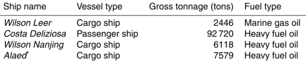
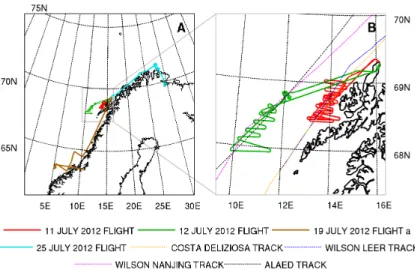
The 4 flights focused on shipping pollution took place on 11, 12, 19 and 25 July 2012 and are shown in Fig. 1a (zoom in on the 11 and 12 July 2012 flights shown in Fig. 1b). The 3 flights on 11, 12 and 25 July 2012 sampled pollution from specific ships (referred

15

to as single-plume flights). During these flights, the research aircraft repeatedly sam-pled relatively fresh emissions from one or more ships during flight legs at constant altitudes, at several distances from the emission source, and in some cases at diff er-ent altitudes. In this study, measuremer-ents from these single plume flights are used in combination with ship plume dispersion simulations (described in Sects. 3.1 and 4.1)

20

to estimate emissions from individual ships. This method relies on knowing the precise locations of the ships during sampling. Because those locations are not known for the ship emissions sampled on 25 July 2012 flight, emissions are only calculated for the 3 ships targeted during the 11 and 12 July flights (theCosta Deliziosa,Wilson Leer

andWilson Nanjing), and for an additional ship (theAlaed) sampled during the 12 July

25

(8)

ACPD

15, 18407–18457, 2015

L. Marelle et al.

Title Page

Tables Figures

◭ ◮

Back Close

Full Screen / Esc

Discussion

P

a

per

|

Discussion

P

a

per

|

Discussion

P

a

per

|

Discussion

P

a

per

|

sampled fresh ship emissions within the boundary layer, during flight legs at low alti-tudes (<200 m). Fresh ship emissions were sampled less than 4 h after emission. In addition to the single plume flights, the 19 July 2012 ACCESS flight targeted aged ship emissions in the marine boundary layer near Trondheim. Data collected during these 4 flights are used to derive emissions from operating ships and to evaluate regional

5

chemical transport simulations investigating the impacts of shipping in northern Nor-way. Other flights from the ACCESS campaign were not used in this study because their flight objectives biased the measurements towards other emissions sources (e.g. oil platforms in the Norwegian Sea) or because they included limited sampling in the boundary layer (flights north to Svalbard and into the Arctic free troposphere, Roiger

10

et al., 2015).

3 Modeling tools

3.1 FLEXPART-WRF and WRF

Plume dispersion simulations are performed with FLEXPART-WRF for the 4 ships pre-sented in Table 1, in order to estimate their emissions of NO_x and SO₂.

FLEXPART-15

WRF (Brioude et al., 2013) is a version of the Lagrangian particle dispersion model FLEXPART (Stohl et al., 2005), driven by meteorological fields from the mesoscale weather forecasting model WRF (Skamarock et al., 2008). In order to drive FLEXPART-WRF, a meteorological simulation was performed with WRF version 3.5.1, from 4 to 25 July 2012, over the domain presented in Fig. 1a. The domain (15 km×15 km horizontal 20

resolution with 65 vertical eta levels between the surface and 50 hPa) covers most of northern Norway (_∼62 to 75◦_{N) and includes the region of all ACCESS flights focused}

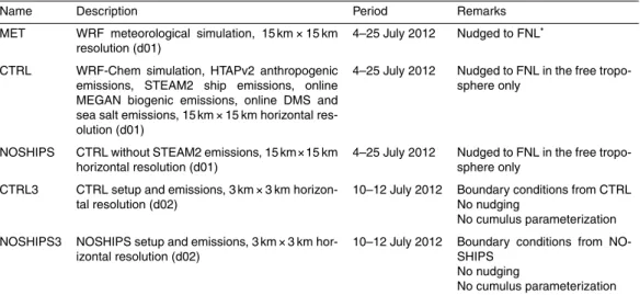
on ship emissions. The first week of the simulation (4 to 10 July included) is used for model spin up. WRF options and parameterizations used in these simulations are shown in Table 2. Meteorological initial and boundary conditions are obtained from the

25

final (FNL) analysis from NCEP (National Centers for Environmental Prediction). The

(9)

ACPD

15, 18407–18457, 2015

L. Marelle et al.

Title Page

Tables Figures

◭ ◮

Back Close

Full Screen / Esc

Discussion

P

a

per

|

Discussion

P

a

per

|

Discussion

P

a

per

|

Discussion

P

a

per

|

simulation is also nudged to FNL winds, temperature and humidity every 6 h. This WRF meteorological simulation is referred to as the MET simulation.

Moving ship emissions are represented in the FLEXPART-WRF plume dispersion simulations as moving 2 m×2 m×2 m box sources, whose locations are updated every

10 s along the ship trajectory (routes shown on Fig. 1b). 1000 particles are released

5

every 10 s into these volume sources, representing a constant emission flux with time of an inert tracer. During the ACCESS flights, targeted ships were moving at relatively constant speeds during the∼3 h of the flight, meaning that fuel consumption and

emis-sion fluxes are likely to be constant during the flights if environmental conditions (wind speed, waves and currents) were not varying strongly. FLEXPART-WRF takes into

ac-10

count a simple exponential decay using a prescribed lifetime. In our case, the lifetime of NO_x relative to their reaction with OH was estimated using results from WRF-Chem simulations presented in Sect. 3.2. Specifically, we use OH concentrations, tempera-ture and air density from the CTRL3 simulation (see Sects. 3.2 and 5.1). The NO_x life-time was estimated to be 12 h on 11 July, 5 h on 12 July. The SO₂lifetime was not taken

15

into account, consistent with the findings of Lee et al. (2011), who reported a lifetime of

∼20 h over the mid-Atlantic during summer, which is significantly longer than the ages

of plumes measured during ACCESS. The FLEXPART-WRF output consists of parti-cle positions, each associated with a pollutant mass; these partiparti-cles are mapped onto a 3-D output grid (600 m×600 m, with 18 vertical levels between 0 and 1500 m a.s.l.) 20

to derive fields of volume mixing ratios every minute. Since emissions are assumed to be constant with time and since our simulations only take into account transport pro-cesses depending linearly on concentrations, the intensity of these mixing ratio fields also depend linearly on the emission strength chosen for the simulation. Therefore, the model results can be scaled a posteriori to represent any constant emission flux value.

25

(10)

ACPD

15, 18407–18457, 2015

L. Marelle et al.

Title Page

Tables Figures

◭ ◮

Back Close

Full Screen / Esc

Discussion

P

a

per

|

Discussion

P

a

per

|

Discussion

P

a

per

|

Discussion

P

a

per

|

and wind speed, as well as the volume flow rate and temperature at the ship exhaust, to calculate a plume injection height above the ship stack. Ambient temperature and wind speed values at each ship’s position are obtained from the WRF simulation. We use an average of measurements by Lyyranen et al. (1999) and Cooper (2001) as the exhaust temperature of the 4 targeted ships (350◦_{C). The volume flows at the}

ex-5

haust are derived for each ship using CO₂emissions from the STEAM2 ship emission model (STEAM 2 emissions described in Sect. 3.3). Specifically, CO₂ emissions from STEAM2 for the 4 targeted ships are converted to an exhaust gas flow based on the average composition of ship exhaust gases measured by Cooper (2001) and Petzold et al. (2008). Average injection heights, including stack heights and plume rise, are

10

found to be approximately 230 m for theCosta Deliziosa, 50 m for theWilson Nanjing, 30 m for theWilson Leerand 65 m for theAlaed. In order to estimate the sensitivity of plume dispersion to these calculated injection heights, two other simulations are per-formed for each ship, where injection heights are decreased and increased by 50 %. Details of the FLEXPART-WRF runs and how they are used to estimate emissions are

15

presented in Sect. 4.

3.2 WRF-Chem

In order to estimate the impacts of shipping on air quality and radiative e_ffects in north-ern Norway, simulations are performed using the 3-D chemical transport WRF-Chem (Weather Research and Forecasting model, including chemistry, Grell et al., 2005; Fast

20

et al., 2006). WRF-Chem has been used previously by Molders et al. (2010) to quantify the influence of ship emissions on air quality in southern Alaska. Table 2 summarizes all the WRF-Chem options and parameterizations used in the present study, detailed briefly below. The gas phase mechanism is the carbon bond mechanism, version Z (CBM-Z, Zaveri and Peters, 1999). The version of the mechanism used in this study

25

includes dimethylsulfide (DMS) chemistry. Aerosols are represented by the 8 bin sec-tional MOSAIC (Model for Simulating Aerosol Interactions and Chemistry, Zaveri et al., 2008) mechanism. Aerosol optical properties are calculated by a Mie code within

(11)

ACPD

15, 18407–18457, 2015

L. Marelle et al.

Title Page

Tables Figures

◭ ◮

Back Close

Full Screen / Esc

Discussion

P

a

per

|

Discussion

P

a

per

|

Discussion

P

a

per

|

Discussion

P

a

per

|

Chem, based on the simulated aerosol composition, concentrations and size distribu-tions. These optical properties are linked with the radiation modules (aerosol direct effect), and this interaction also modifies the modeled dynamics and can affect cloud formation (semi-direct effect). The simulations also include cloud/aerosol interactions, representing aerosol activation in clouds, aqueous chemistry for activated aerosols,

5

and wet scavenging within and below clouds. Aerosol activation changes the cloud droplet number concentrations and cloud droplet radii in the Morrison microphysics scheme, thus influencing cloud optical properties (first indirect aerosol e_ffect). Aerosol activation in MOSAIC also influences cloud lifetime by changing precipitation rates (second indirect aerosol effect).

10

Chemical initial and boundary conditions are taken from the global chemical-transport model MOZART-4 (model for ozone and related chemical tracers version 4, Emmons et al., 2010). In our simulations, the dry deposition routine for trace gases (Wesely, 1989) was modified to improve dry deposition on snow, following the recom-mendations of Ahmadov et al. (2015). The seasonal variation of dry deposition was

15

also updated to include a more detailed dependence of dry deposition parameters on land use, latitude and date, which was already in use in WRF-Chem for the MOZART-4 gas-phase mechanism. Anthropogenic emissions (except ships) are taken from the HTAPv2 (Hemispheric transport of air pollution, version 2) inventory (0.1◦×0.1◦

res-olution). Bulk VOCs are speciated using emission profiles for the UK from Murrels

20

et al. (2010). DMS emissions are calculated following the methodology of Nightingale et al. (2000) and Saltzman et al. (1993). The oceanic concentration of DMS in the Nor-wegian Sea in July, taken from Lana et al. (2011) is 5.8×10−6mol m−3. Other biogenic

emissions are calculated online by the MEGAN model (Guenther et al., 2006) within WRF-Chem. Sea salt emissions are also calculated online within WRF-Chem.

25

(12)

ACPD

15, 18407–18457, 2015

L. Marelle et al.

Title Page

Tables Figures

◭ ◮

Back Close

Full Screen / Esc

Discussion

P

a

per

|

Discussion

P

a

per

|

Discussion

P

a

per

|

Discussion

P

a

per

|

simulations are carried out from 4 to 26 July 2012, over the 15 km×15 km simulation

domain presented in Fig. 1a. The CTRL3 and NOSHIPS3 simulations are similar to CTRL and NOSHIPS, but are run on a smaller 3 km×3 km resolution domain, shown

in Fig. 1b, from 10 to 13 July 2012. The CTRL3 and NOSHIPS3 simulations are not nudged to FNL and do not include a subgrid parameterization for cumulus due to their

5

high resolution. Boundary conditions for CTRL3 and NOSHIPS3 are taken from the CTRL and NOSHIPS simulations (using one way nesting within WRF-Chem) and are updated every hour.

The CTRL and CTRL3 simulations are not nudged to the reanalysis fields in the boundary layer, in order to obtain a more realistic boundary layer structure. However,

10

comparison with ACCESS meteorological measurements shows that on 11 July 2012 this leads to an overestimation of marine boundary layer wind speeds (normalized mean bias= +38 %). Since wind speed is one of the most critical parameters in the FLEXPART-WRF simulations, we decided to drive FLEXPART-WRF with the MET simu-lation instead of using CTRL or CTRL3. In the MET simusimu-lation, results are also nudged

15

to FNL in the boundary layer in order to reproduce wind speeds (normalized mean bias of₊14 % on 11 July 2012). All CTRL, NOSHIPS, CTRL3, NOSHIPS3 and MET sim-ulations agree well with meteorological measurements during the other ACCESS ship flights.

3.3 High resolution ship emissions from STEAM2

20

STEAM2 is a high resolution, real time bottom-up shipping emissions model based on AIS positioning data (Jalkanen et al., 2012). STEAM2 calculates fuel consumption for each ship based on its speed, engine type, fuel type, vessel length, and propeller type. The model can also take into account the e_ffect of waves, and distinguishes ships at berth, maneuvering ships and cruising ships. Contributions from weather e_ffects were

25

not included in this study, however. The presence of AIS transmitters is mandatory for large ships (gross tonnage>300 t) and voluntary for smaller ships.

(13)

ACPD

15, 18407–18457, 2015

L. Marelle et al.

Title Page

Tables Figures

◭ ◮

Back Close

Full Screen / Esc

Discussion

P

a

per

|

Discussion

P

a

per

|

Discussion

P

a

per

|

Discussion

P

a

per

|

Emissions from STEAM2 are compared with emissions derived from measurements for individual ships in Sect. 4. STEAM2 emissions of CO, NO_x, OC, BC (technically elemental carbon in STEAM2), sulfur oxides (SO_x), SO₄, and exhaust ashes are also used in the WRF-Chem CTRL and CTRL3 simulations. SO_x are emitted as SO₂ in WRF-Chem, and NO_x are emitted as 94 % NO, 6 % NO₂ (EPA, 2000). VOC

emis-5

sions are estimated from STEAM2 CO emissions using a bulk VOC/CO mass ratio of 53.15 %, the ratio used in the Arctic ship inventory from Corbett et al. (2010). STEAM2 emissions were generated on a 5 km_×5 km grid every 30 min for the CTRL simulation, and on a 1 km×1 km grid every 15 min for the CTRL3 simulation, and were regridded

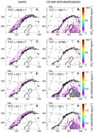
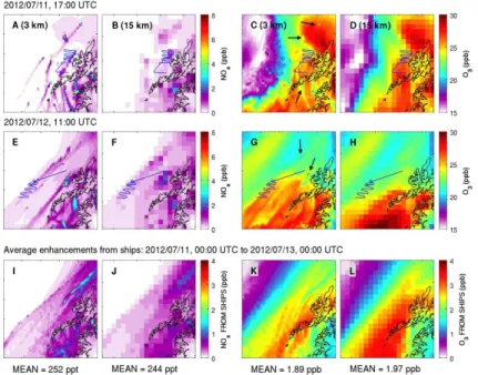
on the WRF-Chem simulation grids. Shipping emissions of NO_x, SO₂, black carbon,

10

and organic carbon are presented in Fig. 2 for the 15 km×15 km simulation domain

(emissions totals during the simulation period are indicated within the figure panels). For comparison, the HTAPv2 emissions (without shipping emissions) are also shown. Ship emissions are, on average, located in main shipping lanes along the Norwegian coastline. However, they also include less traveled routes, which are apparent closer to

15

shore. Other anthropogenic emissions are mainly located along the Norwegian coast (mostly in southern Norway) or farther inland and to the south in Sweden and Finland. Over the whole domain, NO_x and OC emissions from shipping are approximately one third of total anthropogenic NO_x and OC emissions, but represent a lower proportion of anthropogenic SO₂ and BC emissions (5 and 10 %, respectively). However, other

20

anthropogenic emissions are not co-located with shipping emissions, which represent an important source further north along the coast, as many ships are in transit be-tween European ports and Murmansk in Russia. Very strong SO₂emissions in Russia are included in the model domain, associated with smelting activities that occur on the Russian Kola Peninsula (Fig. 2d, Virkkula et al., 1997; Prank et al., 2010).

25

(14)

gener-ACPD

15, 18407–18457, 2015

L. Marelle et al.

Title Page

Tables Figures

◭ ◮

Back Close

Full Screen / Esc

Discussion

P

a

per

|

Discussion

P

a

per

|

Discussion

P

a

per

|

Discussion

P

a

per

|

ated along the Norwegian coast. As a result, ship emissions in the northern Baltic and along the northwestern Russian coast are not included in this study. However, these missing shipping emissions are much lower than other anthropogenic sources inside the model domain. Ship emissions are injected in altitude using the plume rise model presented in Sect. 3.1 in the CTRL and CTRL3 simulations. Stack height and exhaust

5

fluxes are unknown for most of the ships present in the STEAM2 emissions, which were not specifically targeted during ACCESS. For these ships, exhaust parameters for the

Wilson Leer(∼6000 gross tonnage) are used as a compromise between the smaller

fishing ships (∼40 % of Arctic shipping emissions, Winther et al., 2014), and larger

ships like the ones targeted during ACCESS. In the CTRL3 simulation, the 4 ships

tar-10

geted during ACCESS are usually alone in a 3 km×3 km grid cell, which enabled us to

treat these ships separately and to inject them in altitude using their individual exhaust parameters (Sect. 3.1). In the CTRL simulation, there are usually several ships in the same 15 km×15 km grid cell, and the 4 targeted ships were treated in the same way

together with all unidentified ships, using the exhaust parameters of the Wilson Leer 15

and local meteorological conditions to estimate injection heights.

Primary aerosol emissions from STEAM2 (BC, OC, SO₄ and ash) are distributed into the 8 MOSAIC aerosol bins in WRF-Chem, according to the mass size distribu-tion measured in the exhaust of ships equipped with medium-speed diesel engines by Lyyranen et al. (1999). The submicron mode of this measured distribution is used

20

to distribute primary BC, OC and SO=₄, while the coarse mode is used to distribute exhaust ash particles (represented as “other inorganics” in MOSAIC).

4 Ship emission evaluation

In this section, emissions of NO_xand SO₂are determined for the 4 ships sampled dur-ing ACCESS flights (shown in Table 1). First, we compare airborne measurements in

25

ship plumes and concentrations predicted by FLEXPART-WRF plume dispersion sim-ulations. In order to derive emission fluxes, good agreement between measured and

(15)

ACPD

15, 18407–18457, 2015

L. Marelle et al.

Title Page

Tables Figures

◭ ◮

Back Close

Full Screen / Esc

Discussion

P

a

per

|

Discussion

P

a

per

|

Discussion

P

a

per

|

Discussion

P

a

per

|

modeled plume locations is required (discussed in Sect. 4.1). The methods, derived emissions values for the 4 ships, and comparison with STEAM2 emissions, are pre-sented in Sect. 4.2.

4.1 Ship plume representation in FLEXPART-WRF and comparison with

airborne measurements

5

FLEXPART-WRF plume dispersion simulations driven by the MET simulation are per-formed for the 4 ships sampled during ACCESS (Sect. 3.1). The MET simulation agrees well with airborne meteorological measurements on both days in terms of wind direc-tion (mean bias of₋16◦_{on 11 July,}

+6◦_{on 12 July) and wind speed (normalized mean}

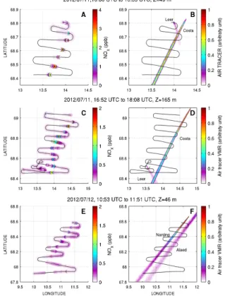
bias of+14 % on 11 July,−17 % on 12 July). Figure 3 shows the comparison between 10

maps of the measured NO_x and plume locations predicted by FLEXPART-WRF. This figure also shows the typical meandering pattern of the plane during ACCESS, mea-suring the same ship plumes several times as they age, while moving further away from the ship (Roiger et al., 2015). Modeled and measured plume locations agree well for all ships.Wilson LeerandCosta Deliziosaplumes were sampled during two di_ff

er-15

ent runs at two altitudes on 11 July 2012, and presented in Fig. 3a and b (z=49 m) and Fig. 3c and d (z=165 m). During the second altitude level on 11 July (Fig. 3c and d) theWilson Leer was farther south and theCosta Deliziosa had moved further north. Therefore, the plumes are farther apart than during the first pass at 49 m. On 12 July 2012, the aircraft targeted emissions from theWilson Nanjingship (Fig. 3e and

20

f), but also sampled the plume of another ship, theAlaed. This last ship was identified during the post-campaign analysis, and we were able to extract its location and emis-sions from the STEAM2 inventory in order to perform the plume dispersion simulations shown here. The NO_x and FLEXPART-WRF predicted plume locations are again in good agreement for both ships.

25

(16)

meander-ACPD

15, 18407–18457, 2015

L. Marelle et al.

Title Page

Tables Figures

◭ ◮

Back Close

Full Screen / Esc

Discussion

P

a

per

|

Discussion

P

a

per

|

Discussion

P

a

per

|

Discussion

P

a

per

|

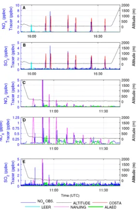
ing pattern before turning around for an additional plume crossing. As expected from the comparison shown in Fig. 3, modeled peaks are co-located with measured peaks in Fig. 4. The model is also able to reproduce the gradual decrease of concentrations measured in the plume of the Wilson Nanjingon Fig. 4c–e, as the plane flies further away from the ship and the plume gets more dispersed. These peak concentrations

5

vary less for the measured and modeled plume of theCosta Deliziosa(Fig. 4a and b). Measured plumes are less concentrated for theWilson Leersince it is a smaller vessel, and for theAlaedbecause its emissions were sampled further away from their source.

4.2 Ship emission derivation and comparison with STEAM2

In this section, we describe the method for deriving ship emissions of NO_x and SO₂

10

using FLEXPART-WRF and measurements. This method relies on the fact that in the FLEXPART-WRF simulations presented in Sect. 3.1, there is a linear relationship be-tween the constant emission flux of tracer chosen for the simulation and the tracer concentrations in the modeled plume. In our simulations, this constant emission flux is picked atE =0.1 kg s−1 _{and is identical for all ships. This initial value} _E _{is scaled for}

15

each ship by the ratio of the measured and modeled areas of the peaks in concen-tration corresponding to plume crossings, as shown in Fig. 4. Equation (1) shows how SO₂emissions are derived by this method.

E_i =E×

Rtend

i

t_ibegin(SO2(t)−SO2background) dt Rtend

i

t_ibeginTracer(t)dt

×

MSO₂

M_air (1)

In Eq. (1), SO₂(t) is the measured SO₂mixing ratio (ppt), SO₂background is the

back-20

ground SO₂ mixing ratio for each peak, Tracer(t) is the modeled tracer mixing ratio interpolated along the ACCESS flight track (ppt),t_ibeginandtend_i are the beginning and end time of peak i (modeled or measured, in s) and MSO₂ and Mair are the molar

(17)

ACPD

15, 18407–18457, 2015

L. Marelle et al.

Title Page

Tables Figures

◭ ◮

Back Close

Full Screen / Esc

Discussion

P

a

per

|

Discussion

P

a

per

|

Discussion

P

a

per

|

Discussion

P

a

per

|

masses of SO₂ and air (kg m−3_{). This method produces a di}

fferent E_i SO₂ emission flux value (kg s−1) for each of thei =1 toN peaks corresponding to all the crossings of a single ship plume by the aircraft. TheseN different estimates are averaged together to reduce the uncertainty in the estimated SO₂emissions. A similar approach is used to estimate NO_xemissions.

5

In order to reduce sensitivity to the calculated emission injection heights, FLEXPART-WRF peaks that are sensitive to a_±50 % change in injection height are excluded from the analysis. Results are considered sensitive to injection heights if the peak area in tracer concentration changes by more than 50 % in the injection height sensitivity runs. Using a lower threshold of 25 % alters the final emission estimates by less than 6 %.

10

Peaks sensitive to the calculated injection height typically correspond to samplings close to the ship, where the plumes are narrow. An intense SO₂peak most likely asso-ciated with theCosta Deliziosaand sampled around 17:25 UTC on 11 July 2012 is also excluded from the calculations, because this large increase in SO₂in an older, diluted part of the ship plume suggests contamination from another source. SO₂emissions are

15

not determined for the Wilson Leerand theAlaed, since SO₂ measurements in their plumes are too low to be distinguished from the background variability. For the same reason, only the higher SO₂ peaks (4 peaks>1 ppb) were used to derive emissions for theWilson Nanjing. The number of peaks used to derive emissions for each ship is

N=13 for theCosta Deliziosa,N=4 for theWilson Leer,N=8 for theWilson Nanjing 20

(N=4 for SO₂) andN=5 for theAlaed.

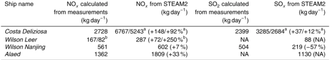
The derived emissions of NO_x (equivalent NO₂ mass flux in kg day−1_{) and SO}

2 are

given in Table 4. The emissions extracted from the STEAM2 inventory for the same ships during the same time period are also shown. STEAM2 SO₂emissions are higher than the value derived for the Costa Deliziosa, and lower than the value derived for

25

(18)

re-ACPD

15, 18407–18457, 2015

L. Marelle et al.

Title Page

Tables Figures

◭ ◮

Back Close

Full Screen / Esc

Discussion

P

a

per

|

Discussion

P

a

per

|

Discussion

P

a

per

|

Discussion

P

a

per

|

quired value. For theWilson Leer, two calculated values are reported: one calculated by averaging the estimates from the 4 measured peaks, and one value where an outlier value was removed before calculating the average. During the 11 July flight, theWilson Leerwas traveling south at an average speed of 4.5 m s−1, with relatively slow tailwinds of 5.5 m s−1. Because of this, the dispersion of this ship’s plume on this day could be

5

sensitive to small changes in modeled wind speeds, and calculated emissions are less certain.

The most important difference between the inventory NO_x and our estimates is

∼150 % for theCosta Deliziosa. Reasons for large discrepancy in predicted and

mea-sured NO_x emissions ofCosta Deliziosawere investigated in more detail. A complete

10

technical description ofCosta Deliziosa was not available, but her sister vesselCosta Luminosawas described at length recently (RINA, 2010). The details ofCosta Lumi-nosaandCosta Deliziosaare practically identical and allow in-depth analysis of emis-sion modeling. With complete technical data, the STEAM2 SO_x and NO_xemissions of

Costa Deliziosawere estimated to be 2684 and 5243 kg day−1_{, respectively, whereas}

15

our derived estimates indicate 2399 and 2728 kg day−1 _(di

fference of₊12 % for SO_x and+92 % for NO_x). The good agreement for SO_x indicates that the power prediction at vessel speed reported in AIS and associated fuel flow is well predicted by STEAM2, but emissions of NO_x are twice as high as the value derived from measurements. In case ofCosta Deliziosa, the NO_xemission factor of 10.5 g kWh−1_{for a Tier II compliant} 20

vessel with 500 RPM engine is assumed by STEAM2. Based on the measurements-derived value, a NO_x emission factor of 5.5 g kWh−1_{would be necessary, which is well}

below the Tier II requirements. It was reported recently (IPCO, 2015), that NO_x emis-sion reduction technology was installed on Costa Deliziosa, but it is unclear whether this technology was in place during the airborne measurement campaign in 2012.

25

The case ofCosta Deliziosaunderlines the need for accurate and up-to-date techni-cal data for ships when bottom-up emission inventories are constructed. It also neces-sitates the inclusion of the e_ffect of emission abatement technologies in ship emission inventories. Furthermore, model predictions for individual vessels are complicated by

(19)

ACPD

15, 18407–18457, 2015

L. Marelle et al.

Title Page

Tables Figures

◭ ◮

Back Close

Full Screen / Esc

Discussion

P

a

per

|

Discussion

P

a

per

|

Discussion

P

a

per

|

Discussion

P

a

per

|

external contributions, like weather and sea currents, affecting vessel performance. A recent study by Beecken et al. (2014) compared STEAM2 NO_x, SO₂ and PM emis-sion factors to estimates based on airborne measurements for∼300 ships in the Baltic

Sea and found, on average, no strong bias in STEAM2 predictions of NO_x. In Beecken et al. (2014) the emission factors of SOx and PM were shown to deviate from

measure-5

ments mainly because of the differences in assumed and measured fuel sulfur content. Regardless of the differences, regional emission inventories generated by STEAM2 can describe the geographical distribution of ship emissions accurately. The results presented later in Sect. 5.1 indicate that this is also likely true in the Norwegian Sea during ACCESS, despite the uncertainties for individual ships.

10

4.3 Comparison of STEAM2 to other shipping emission inventories for

northern Norway

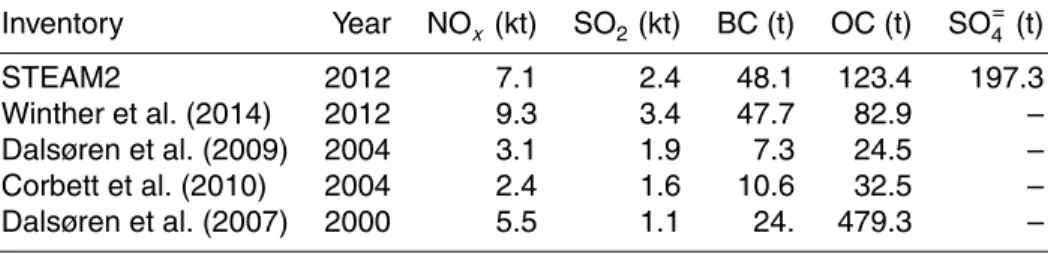
We compare in Table 5 the July emission totals for NO_x, SO₂, BC, OC and SO=₄ in northern Norway (latitudes 60.6 to 73◦N, longitudes 0 to 31◦W) for STEAM2 and 4 other shipping emission inventories used in previous studies investigating shipping

im-15

pacts in the Arctic. We include emissions from the Winther et al. (2014), Dalsøren et al. (2009, 2007) and Corbett et al. (2010) inventories. The highest shipping emissions in the region of northern Norway are found in the STEAM2 and Winther et al. (2014) inventories, which are both based on 2012 AIS ship activity data (see Sect. 3.3 for a description of the methodology used for STEAM2). We note that, except for OC,

20

the emissions are higher in the Winther et al. (2014) inventory because of the larger geographical coverage: Winther et al. (2014) used both ground based and satellite re-trieved AIS signals, whereas the current study is restricted to data received by ground based AIS stations (capturing ships within 50 to 90 km of the Norwegian coastline). Despite lower coverage, the horizontal and temporal resolutions are better described

25

(20)

in-ACPD

15, 18407–18457, 2015

L. Marelle et al.

Title Page

Tables Figures

◭ ◮

Back Close

Full Screen / Esc

Discussion

P

a

per

|

Discussion

P

a

per

|

Discussion

P

a

per

|

Discussion

P

a

per

|

ventory including sulfate emissions, which account for SO₂ to SO=₄ conversion in the ship exhaust. Ship emissions from Dalsøren et al. (2009) and Corbett et al. (2010) are based on ship activity data from 2004, when marine tra_ffic was lower than in 2012. Fur-thermore, the gridded inventory from Corbett et al. (2010) does not include emissions from fishing ships, which represent close to 40 % of Arctic shipping emissions (Winther

5

et al., 2014). These emissions could not be precisely distributed geospatially using ear-lier methodologies, since fishing ships do not typically follow a simple course (Corbett et al., 2010). Dalsøren et al. (2007) emissions for coastal shipping in Norwegian waters are estimated based on Norwegian shipping statistics for the year 2000, and contain higher NO_x, BC and OC emissions, but less SO₂, than the 2004 inventories. This

com-10

parison indicates that earlier ship emission inventories usually contain lower emissions in this region, which can be explained by the current growth in shipping tra_ffic in north-ern Norway. This means that up-to-date emissions are required in order to assess the current impacts of shipping in this region.

5 Modeling the impacts of ship emissions along the Norwegian coast

15

In this section, WRF-Chem using STEAM2 ship emissions is employed to study the influence of ship pollution on atmospheric composition along the Norwegian coast, at both the local and regional scale. As shown in Fig. 4, shipping pollution measured dur-ing ACCESS is inhomogeneous, with sharp NO_x and SO₂peaks in thin ship plumes, emitted into relatively clean background concentrations. The measured concentrations

20

are on spatial scales that can only be reproduced using very high-resolution WRF-Chem simulations (a few kms of horizontal resolution), but such simulations can only be performed for short periods and over small domains. Therefore, high-resolution sim-ulations cannot be used to estimate the regional impacts of shipping emissions. In order to bridge the scale between measurements and model runs that can be used

25

to make conclusions about the regional impacts of shipping pollution, we compare in Sect. 5.1 WRF-Chem simulations using STEAM2 ship emissions, at 3 km_×3 km

(21)

ACPD

15, 18407–18457, 2015

L. Marelle et al.

Title Page

Tables Figures

◭ ◮

Back Close

Full Screen / Esc

Discussion

P

a

per

|

Discussion

P

a

per

|

Discussion

P

a

per

|

Discussion

P

a

per

|

tion (CTRL3) and at 15 km×15 km resolution (CTRL). Specifically, we show in Sect. 5.1

that both the CTRL3 and CTRL simulations reproduce the average regional influence of ships on NO_x, O₃and SO₂, compared to ACCESS measurements. In Sect. 5.2 we use the CTRL simulation to quantify the regional contribution of ships to surface pollution and shortwave radiative fluxes in northern Norway.

5

5.1 Local impacts of ship emissions and influence of model resolution

It is well known that ship plumes contain fine scale features that cannot be captured by most regional or global chemical transport models. This fine plume structure influ-ences the processing of ship emissions, including O₃and aerosol formation, which are non-linear processes that largely depend on the concentration of species inside the

10

plume. Some models take into account the influence of the instantaneous mixing of ship emissions in the model grid box by including corrections to the O₃production and destruction rates (Huszar et al., 2010) or take into account plume ageing before dilution by using corrections based on plume chemistry models (Vinken et al., 2011). Here, we take an alternative approach by running the model at a su_fficient resolution to

distin-15

guish individual ships in the Norwegian Sea (CTRL3 run at 3 km×3 km resolution), and

at a lower resolution (CTRL run at 15 km×15 km resolution). The CTRL and CTRL3

simulations (see Table 3) are compared to evaluate if nonlinear e_ffects are important in this case. We also evaluate the ability of WRF-Chem simulations with STEAM2 emis-sions to distinguish individual ship plumes and to predict their composition.

20

WRF-Chem results from CTRL and CTRL3 for surface (∼0 to 30 m) NOx and O3

are shown in Fig. 5. On 11 and 12 July, the Falcon 20 specifically targeted plumes from theWilson Leer,Costa Deliziosa,Wilson Nanjingand, in addition, sampled emis-sions from theAlaed, identified later during the post-campaign analysis (see Fig. 3). All these ships are individually present in the STEAM2 emissions inventory (see Sect. 4

25

(22)

ACPD

15, 18407–18457, 2015

L. Marelle et al.

Title Page

Tables Figures

◭ ◮

Back Close

Full Screen / Esc

Discussion

P

a

per

|

Discussion

P

a

per

|

Discussion

P

a

per

|

Discussion

P

a

per

|

individual ship plumes cannot be clearly distinguished in the NO_x surface concentra-tions. The predicted surface O₃ concentrations are shown in Fig. 5c, d, g, and h. On the 11 and 12 July 2012, titration of O₃by NO from fresh ship emissions can be iden-tified in Fig. 5c and g for the 3 km run (areas indicated by black arrows on Fig. 5c and g). However, evidence for O₃titration quickly disappears away from the fresh emissions

5

sources. In contrast, O₃titration is not apparent in the CTRL run. However, NO_xand O₃ patterns and average surface concentrations are very similar. This is illustrated in the lower panels, showing 2-day averaged NO_x and O₃enhancements due to ships in the CTRL3 (CTRL3 – NOSHIPS3) and CTRL (CTRL – NOSHIPS) simulations. The results show that changing the horizontal resolution from 3 km×3 km (1 km×1 km emissions, 10

15 min emissions injection) to 15 km×15 km (5 km×5 km emissions, 1 h emissions

in-jection) does not have a large influence on the domain-wide average NO_x (−3.2 %)

or O₃ (+4.2 %) enhancements due to ships. This is in agreement with earlier results by Cohan et al. (2006), who showed that regional model simulations at similar resolu-tions (12 km) were su_fficient to reproduce the average O₃response. Results by Vinken

15

et al. (2011) suggest that simulations at a lower resolution more typical of global mod-els (2◦

×2.5◦) would lead to an overestimation of O3production from ships in this region

by 1 to 2 ppbv. The influence of model resolution on surface aerosol concentrations is also moderate, and PM₁₀ due to ships are 15 % lower on average in CTRL than in CTRL3 (not shown here).

20

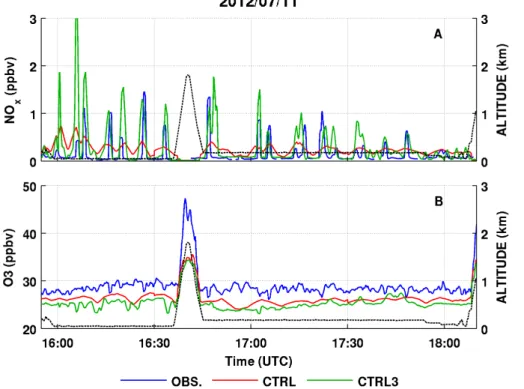
To further investigate the ability of these di_fferent model runs to represent single ship plumes, we compare measured NO_x and O₃along the flight track on 11 July 2012 with WRF-Chem predictions (Fig. 6). Large enhancements of NO_x are seen during plume crossings in measurements, as already noted in Sect. 4. For comparison with WRF-Chem, we have averaged the measured data using a 56 s running average, equivalent

25

to the aircraft crossing 6 km (2 model grid cells) at its average speed during this flight (107 m s−1_{). Using a running average takes into account plume dilution in grid cells, as}

well as additional smoothing introduced when modeled results are spatially interpolated onto the flight track. The CTRL3 simulation captures both the width and magnitude of

(23)

ACPD

15, 18407–18457, 2015

L. Marelle et al.

Title Page

Tables Figures

◭ ◮

Back Close

Full Screen / Esc

Discussion

P

a

per

|

Discussion

P

a

per

|

Discussion

P

a

per

|

Discussion

P

a

per

|

NO_x peaks, suggesting that the individual plumes are correctly represented in space and time. In contrast, the CTRL run has wider NO_x peaks and lower peak heights, because of dilution in larger grids. Both simulations have a tendency to overestimate NO_x in ship plumes, which is in agreement with the results shown in Table 4, indi-cating that STEAM2 NO_x emissions are overestimated for the ships targeted during

5

ACCESS. Figure 6b shows O₃ during the same flight. The CTRL3 simulation repro-duces the ozone variability better than the CTRL run, but both runs perform relatively well on average (mean bias₌₋3 ppbv during the constant altitude legs). Both mea-surements and CTRL3 results show evidence of O₃ titration in the most concentrated NO_xplumes, where ozone is 1.5 to 3 ppbv lower than out of the plumes. However,

pre-10

cise quantification of this titration is di_fficult because these values are the same order of magnitude as the spatial variability of O₃ outside of the plumes. O₃ titration is not apparent in the CTRL run.

In order to evaluate modeled aerosols in ship plumes, modeled aerosols are eval-uated using size distributions measured during the 11 July 2012 flight. Size

distribu-15

tions are integrated to estimate submicron aerosol mass (PM₁), assuming a density of 1700 kg m−3_{and spherical particles. This indicates that observed PM}

1enhancements

in plumes (∼0.1 to 0.5 µg m−3) are relatively low compared to background PM1(∼0.7

to 1.1 µg m−3_{), because of the presence of high sea salt concentrations in the marine}

boundary layer (54 % of the modeled background PM₁ during ship plume sampling is

20

sea salt in NOSHIPS3). Because of this, comparing modeled and observed in-plume PM₁ directly would be mostly representative of background aerosols, especially sea salt, which is not the focus of this paper. Figure 7 shows the comparison between modeled and measured enhancements in PM₁ in the plume of the Costa Deliziosa

(11 July 2012), removing from the model and measurements the contribution from sea

25

(24)

ACPD

15, 18407–18457, 2015

L. Marelle et al.

Title Page

Tables Figures

◭ ◮

Back Close

Full Screen / Esc

Discussion

P

a

per

|

Discussion

P

a

per

|

Discussion

P

a

per

|

Discussion

P

a

per

|

model and the measurements for the first 2 PM₁ plumes measured close to the ships (around 16:05 UTC), which could be an artifact of the limited resolution of this simu-lation (3 km). If these peaks are excluded, the model slightly overestimates peak PM₁ enhancements in ship plumes (+26 %). Since this enhancement is modeled as 80 % SO=₄, this overestimation can be linked to the ₊37 % overestimation of SO₂ emissions

5

for theCosta Deliziosain STEAM2 (see Table 4).

Analysis of O₃maps, average surface enhancements due to ships (Fig. 5) and anal-ysis of model results along flight tracks (Fig. 6) show that both runs capture the NO_x and O₃ concentrations in this region reasonably well. Furthermore, Fig. 7 shows that PM₁enhancements in ship plumes are well reproduced in the CTRL3 simulation, and

10

we found that PM₁₀ production from ships over the simulation domain was not very sensitive to resolution. This suggests that the CTRL simulation is sufficient to assess the impacts of ship emissions at a larger scale during July 2012. This is investigated further by comparing modeled NO_x, SO₂ and O₃ in the CTRL and NOSHIPS simu-lations with the average vertical profiles (100–1500 m) measured during 4 ACCESS

15

flights from 11 to 25 July 2012 (flights shown in Fig. 1a); this comparison is shown in Fig. 8. Modeled vertical profiles of PM_2.5 are also shown in Fig. 8. This comparison allows us to estimate how well CTRL represents the average impact of shipping over a larger area and a longer period.

Figure 8 shows that the NOSHIPS simulation significantly underestimates NO_x and

20

SO₂, and moderately underestimates O₃along the ACCESS flights, indicating that ship emissions are needed to improve the agreement between the model and observations. In the CTRL simulation, NO_x, SO₂ and O₃ vertical structure and concentrations are generally well reproduced, with normalized mean biases of ₊6.9, ₋10.7 and ₋7.5 % respectively. Correlations between modeled (CTRL) and measured profiles are

signifi-25

cant for NO_x and O₃(r2=0.94 and 0.95). The correlation is lower between measured and modeled SO₂ (r2=0.52) but it is improved compared to the NOSHIPS simula-tion (r2=0.35). Ships have the largest influence on NO_x and SO₂profiles, a moderate influence on O₃and do not strongly influence PM_2.5profiles along the ACCESS flights.

(25)

ACPD

15, 18407–18457, 2015

L. Marelle et al.

Title Page

Tables Figures

◭ ◮

Back Close

Full Screen / Esc

Discussion

P

a

per

|

Discussion

P

a

per

|

Discussion

P

a

per

|

Discussion

P

a

per

|

NO_x concentrations are overestimated in the parts of the profile strongly influenced by shipping emissions. This is in agreement with the findings of Sect. 4.2, showing that STEAM2 NO_x emissions were overestimated for the ships sampled during ACCESS. However, the CTRL simulation performs well on average, suggesting that the STEAM2 inventory is able to represent the average emissions from ships along the northern

5

Norwegian coast during the study period. The bias found for SO₂ is especially low compared to the results presented in the multi-model study of Eyring et al. (2007), which showed that global models significantly underestimated SO₂in the polluted ma-rine boundary layer in July. Since aerosols from ships contain mostly secondary sulfate formed from SO₂ oxidation, the validation of modeled SO₂ presented in Fig. 8 gives

10

some confidence in our results compared to earlier studies investigating the air quality and radiative impacts of shipping aerosols. We therefore use the 15 km×15 km CTRL

run for further analysis of the regional influence of ships on pollution and the shortwave radiative e_ffect in this region in Sect. 5.2.

5.2 Regional influence of ship emissions in July 2012

15

5.2.1 Surface air pollution from ship emissions in northern Norway

The regional scale impacts of ships on surface atmospheric composition in northern Norway are estimated by calculating the 15 day (00:00 UTC, 11 July 2012 to 00:00 UTC, 26 July 2012) average difference between the CTRL and NOSHIPS simulations. Fig-ure 9 shows maps of these anomalies at the surface, for NO_x, O₃PM_2.5and BC. Ship

20

emissions have the largest influence on surface NO_x concentrations, with 75 to 100 % increases along the coast. This leads to average O₃increases from shipping of∼6 %

(∼1.5 ppb) in the coastal regions, with slightly lower enhancements (∼1 ppb,∼4 %,)

further inland over Sweden.

Dalsøren et al. (2007) studied the impact of maritime traffic in northern Norway in

25

(26)

How-ACPD

15, 18407–18457, 2015

L. Marelle et al.

Title Page

Tables Figures

◭ ◮

Back Close

Full Screen / Esc

Discussion

P

a

per

|

Discussion

P

a

per

|

Discussion

P

a

per

|

Discussion

P

a

per

|

ever, unlike the present study, the estimate of Dalsoren et al. (2007) did not include the impact of international transit shipping along the Norwegian coast. Our estimated impact on O₃ in this region (6 % and 1.5 ppb increase) is about half of the one deter-mined by Ødemark et al. (2012) (12 % and 3 ppb), for the total Arctic fleet in the sum-mer (JAS) 2004, using ship emissions for the year 2004 from Dalsøren et al. (2009).

5

It is important to note that we expect lower impacts of shipping in studies based on earlier years, because of the continued growth of shipping emissions along the Nor-wegian coast (as discussed in Sect. 4.3, see also Table 5). However, stronger or lower emissions do not seem to completely explain the different modeled impacts. Ødemark et al. (2012) found that Arctic ships had a strong influence on surface O₃ in northern

10

Norway for relatively low 2004 shipping emissions. This could be explained by the dif-ferent processes included in both models, or by different meteorological situations in the two studies based on two different meteorological years (2004 and 2012). How-ever, it is also likely that the higher O₃ in the Ødemark et al. (2012) study could be caused, in part, by nonlinear e_ffects associated with global models running at low

reso-15

lutions. For example Vinken et al. (2011) estimated that instant dilution of shipping NO_x emissions in 2◦

×2.5◦ model grids leads to a 1 to 2 ppb overestimation in ozone in the

Norwegian and Barents seas during July 2005. This e_ffect could explain a large part of the difference in O₃ enhancements from shipping between the simulations of Øde-mark et al. (2012) (2.8◦

×2.8◦ resolution) and the simulations presented in this paper 20

(15 km_×15 km resolution).

The impact on PM_2.5of ships in northern Norway, also shown in Fig. 9., is relatively modest during this period, up to 0.75 µg m−3_{. However, these values correspond to}

an important relative increase of_∼10 % over inland Norway and Sweden because of the low background PM_2.5 in this region. Over the sea surface, the relative effect of

25

ship emissions is quite low because of higher sea salt aerosol background. Aliabadi et al. (2014) have observed similar increases in PM_2.5(0.5 to 1.9 µg m−3_{) in air masses}

influenced by shipping pollution in the remote Canadian Arctic. In spite of the higher tra_ffic in northern Norway, we find lower values because results in Fig. 9 are smoothed