www.biogeosciences.net/7/2581/2010/ doi:10.5194/bg-7-2581-2010
© Author(s) 2010. CC Attribution 3.0 License.
Biogeosciences
A mechanistic account of increasing seasonal variations in the rate
of ocean uptake of anthropogenic carbon
T. Gorgues1, O. Aumont1, and K. B. Rodgers2
1LPO/IRD/CNRS (UMR 6523), centre IRD de Bretagne, Plouzan´e, France
2Atmospheric and Ocean Sciences, Princeton University, Princeton, New Jersey, USA Received: 9 January 2010 – Published in Biogeosciences Discuss.: 29 January 2010 Revised: 15 July 2010 – Accepted: 19 July 2010 – Published: 31 August 2010
Abstract. A three-dimensional circulation model that in-cludes a representation of anthropogenic carbon as a passive tracer is forced with climatological buoyancy and momen-tum fluxes. This simulation is then used to compute offline the anthropogenic1pCO2(defined as the difference between the atmospheric CO2and its seawater partial pressure) trends over three decades between the years 1970 and 2000. It is shown that the mean increasing trends in 1pCO2 reflects an increase of the seasonal amplitude of 1pCO2. In par-ticular, the ocean uptake of anthropogenic CO2 is decreas-ing (negative trends in1pCO2)in boreal (austral) summer in the Northern (Southern) Hemisphere in the subtropical gyres between 20◦N (S) and 40◦N (S). In our simulation, the increased amplitude of the seasonal trends of the1pCO2 is mainly explained by the seasonal sea surface temperature (SST) acting on the anthropogenic increase of the dissolved inorganic carbon (DIC). It is also shown that the seasonality of the anthropogenic DIC has very little effect on the decadal trends. Finally, an observing system forpCO2that is biased towards summer measurements may be underestimating up-take of anthropogenic CO2 by about 0.6 PgC yr−1 globally over the period of the WOCE survey in the mid-1990s ac-cording to our simulations. This bias associated with sum-mer measurements should be expected to grow larger in time and underscores the need for surface CO2measurements that resolve the seasonal cycle throughout much of the extratrop-ical oceans.
Correspondence to:T. Gorgues
(thomas.gorgues@ifremer.fr)
1 Introduction
study of Rodgers et al. (2008) identified seasonal changes in 1pCO2 as accounting for an important component of decadal changes in the North Pacific. However, as the re-analysis fluxes used to force the ocean model in that study included variations on all timescales (storms to decadal), it was not possible there to identify quantitatively specifically the seasonal effect. For that reason, we have chosen here an experimental design where the physical forcing consists of a repeating seasonal cycle over the period of the anthropogenic transient in atmospheric CO2concentration. This allows for a focus specifically on the way in which the anthropogenic transient signal may project itself onto the seasonal cycle in ocean surface conditions.
The primary aim of this present work is to assess the dif-ferent processes responsible for the decadal trends of the an-thropogenic1pCO2 over the global ocean. A parallel aim of this study is to test the hypothesis that an ocean observ-ing network that does not resolve the seasonal cycle in sur-face oceanpCO2will result in significant biases in the rate of uptake of CO2by the ocean. After briefly presenting our method and describing the mean decadal trends in anthro-pogenic1pCO2, our study will focus on the seasonality of these trends. Finally, the processes influencing these trends will be discussed.
2 Method
The model configuration considered here consists of a dy-namical ocean-ice model, and a passive tracer module for the anthropogenic carbon perturbation that is run offline us-ing output from the dynamical model. The dynamical com-ponent is the ORCA2-LIM global coupled ocean-ice model that is based on Version 9 of OPA (Oc´ean PArall´elis´e). OPA is a finite difference model with a free surface and a non-linear equation of state following the formulation of Jackett and McDougall (1995) (Madec and Imbard, 1996; Madec et al., 1998). The domain is global and extends from 78◦S to 90◦N. The bottom topography and coastlines are derived from the study of Smith and Sandwell (1997), complemented by the ETOPO5 data set. Lateral mixing is oriented isopy-cnally, and the eddy parameterization scheme of Gent and McWilliams (1990) is applied poleward of 10◦. Vertical mixing is achieved using the TKE scheme of Blanke and Delecluse (1993).
For the ORCA2 grid configuration, the zonal resolution is 2◦, and meridional resolution ranges from 0.5◦ at the equa-tor to 2◦toward the poles. The model grid is tripolar, with two poles in the Northern Hemisphere (over North America and Siberia) and one centered over Antarctica. The model uses 31 layers in the vertical, with 20 of these layers lying in the upper 500 m. The ocean model is coupled to a sea ice model (Fichefet and Maqueda, 1997; Goosse and Fichefet, 1999). The model was initialized with Boyer et al. (1998) and Antonov et al. (1998) salinity and temperature
climatolo-gies. It was then spun up for 100 years with surface momen-tum forcing fields from a daily mean climatology of wind stress from the ERA40 reanalysis (Uppala et al., 2005).
In this study, only the anthropogenic perturbation of DIC (DICant) and pCO2sw is computed offline using five-day mean circulation fields from the last year of the 100-year spin-up of a circulation model. This representation of the anthropogenic perturbation assumes that the natural (pre-anthropogenic) carbon cycle remained unchanged despite the anthropogenic increase (most importantly, biological fluxes remain stationary in a climatological sense). The anthro-pogenic air-sea CO2fluxes are computed by taking the dif-ference between the carbon fluxes which include the simu-lated perturbation and the natural carbon fluxes. The lat-ter is inferred by reading monthly mean DIC and alka-linity surface fields as provided from a climatological ex-periment using PISCES as described in Aumont and Bopp (2006). The control simulation (hereafter DELC) has been forced by the atmospheric CO2 concentration from 1860 to 2000 (obtained from a spline fit to ice core and Mauna Loa observations, available at http://quercus.igpp.ucla.edu/ OceanInversion/inputs/atm co2/splco2 mod.dat). The car-bonate chemistry follows the OCMIP protocols (see the OCMIP website for more information at www.ipsl.jussieu.fr/ OCMIP) and the gas exchange coefficient is computed from the relationship of Wanninkhof (1992).
In order to identify the relative impacts of seasonal vari-ations of DIC, SST, Alkalinity and Salinity on the1pCO2 trends, we also performed a series of perturbate calculations using monthly and annual mean surface fields from the fully three-dimensional model. The anthropogenic partial pressure of carbon dioxide in the ocean’s surface waters (pCO2sw,ant) is determined by following the protocols of DOE (1994) from dissolved inorganic carbon (DIC), alkalinity, and the disso-ciation constants of carbonic acid. Using these perturbation calculations, we have decoupled the different processes re-sponsible for the anthropogenic1pCO2trends in the global ocean.
3 Results
Fig. 1. (A)Decadal trends in the annual mean of 1pCO2 over 1970–2000 (µatm decade−1)computed from the annual mean of DIC, SST, Alkalinity and Salinity. (B)Decadal trends of1pCO2 for February over 1970–2000 (µatm decade−1)computed from the DIC, SST, Alkalinity and Salinity in February.(C)same as B but for August (i.e. computed from the DIC, SST, Alkalinity and Salinity in August). The numbers in bold green letters indicate the decadal trends of1pCO2computed from Takahashi et al. (2006) and (2009) assuming a 1.5 µatm yr−1increase of the atmospheric CO2 concen-tration over 1970–2000. The values in parenthesis indicate the un-certainty in the same unit. In boxes without parenthesis numbers, uncertainty ranges from 1 to 6 µatm decade−1.
due to the ice sheet that shields the ocean from the anthro-pogenic increase of atmospheric CO2and the emergence of water masses with low anthropogenicpCO2. Local maxima tend to be found along the equatorward and poleward mar-gins of the subtropical gyres, in the polar seas, as well as in the Mediterannean. For the North Pacific, the structures here are consistent with the perturbation structures described in Rodgers et al. (2008). The annual mean as well as the February and August1pCO2trends presented here are also compared with the data analysis presented in the studies of Takahashi et al. (2006, 2009) (Fig. 1). For comparison, we have computed the1pCO2decadal trends from thepCO2sw trends that were considered in those studies. Because the sampling of the data may be biased towards summer, the best agreement is found between the data-based 1pCO2 trends and the model trends for February (Fig. 1b). It has to be noticed that the data-based1pCO2 trends are not directly comparable to our control simulation. Indeed, there are by construction no decadal changes in the physical or biological state of the ocean for our control simulation over the time-period considered in this study. Despite those limitations, the modeled trends are very often in the range of the trends computed from the data published in Takahashi et al. (2006, 2009) when uncertainty is taken into account as well as the sampling bias. It also appears that the trends published in Takahashi et al. (2006 and 2009) show local minima in the center of the subtropical gyres in the Northern Hemisphere, with this also being consistent with our control simulation.
Our main point in this study is to focus on mechanistic un-derstanding through a series of sensitivity studies as a first step towards a more involved interpretation of data. The de-tails of the degree of match or mismatch between the model and the observations should be left as a subject for further investigation, where we will consider a detailed Observing System Simulation Experiment (OSSE).
Figure 1b and c shows the respective decadal trends of sea surface1pCO2 for February and August considered sepa-rately over 1970–2000. In February, the Northern Hemi-sphere displays the same overall pattern (Fig. 1b) seen in the annual mean trend (Fig. 1a), with less pronounced minima in the subtropical gyres. Additionally, the negative decadal trend that was found near the Arctic coast of Russia and in Hudson Bay for the annual mean analysis is more pro-nounced in February. In the Southern Hemisphere, the sub-tropical local minima in February are more pronounced than in the annual mean case.
In August, the Northern Hemisphere summer displays negative1pCO2trends in the subtropical gyres for both the Pacific and Atlantic basins (Fig. 1c). The minima in the
annual mean (Fig. 1a) but with less pronounced minima in the subtropical gyre (Fig. 1c).
The decadal trend towards an increased mean annual uptake of anthropogenic CO2 over the period 1970–2000 (Fig. 1a) is then the result of a global increase of the anthro-pogenic1pCO2maximum in winter (boreal in the Northern Hemisphere and austral in the Southern Hemisphere) offset-ting a slight decrease of the1pCO2 in summer (boreal in the Northern Hemisphere and austral in the Southern Hemi-sphere) (Fig. 1b–c). Thus, the mean annual increased uptake of anthropogenic CO2is in fact accompanied by an increase in the seasonal variability of the1pCO2.
With this analysis of decadal1pCO2trends for winter and summer seasons considered separately for a repeating sea-sonal cycle in the physical state of the ocean, the most sur-prising aspect is thatpCO2sw in the subtropical gyres and in the Northern Hemisphere high latitudes tends to increase more rapidly thanpCO2atm. Why does this occur? In order to address the underlying mechanism, we performed a series of perturbation calculations. The partial pressure of anthro-pogenic CO2at the ocean surface (pCO2sw,ant)is computed using the monthly and annual mean output of modeled DIC, SST, sea surface salinity (SSS) and surface alkalinity using the method prescribed in DOE (1994). With all fields varying monthly, this perturbation method is able to reproduce well the evolution of1pCO2obtained with the control simulation (not shown).
In order to identify the relative impacts of seasonal vari-ations in surface DIC concentrvari-ations, SST, alkalinity, and salinity on the decadal trends in the seasonal cycle of
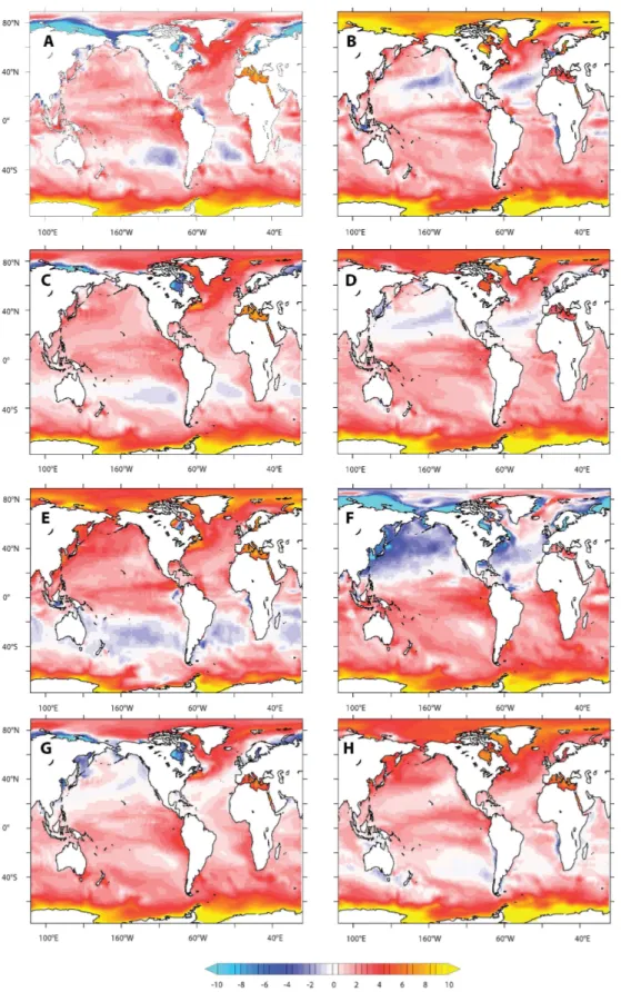
1pCO2, a series of perturbation calculations were performed where one of these fields was maintained at its annual mean value while the others were allowed to vary seasonally. The resulting decadal1pCO2trends for February are shown in the first column of Fig. 2, and for August are shown in the second column. The case with annual mean alkalinity is henceforth referred to as MALK, the case with annual mean salinity as MSAL, the case with annual mean DIC as MDIC, and the case with annual mean SST as MSST.
We begin in Fig. 2 with a comparison of both the MALK (Fig. 2a–b) and MSAL (Fig. 2c–d) cases with our control simulation (Fig. 1b–c). In the Northern Hemisphere high lat-itudes (the Arctic coast of Russia and the Hudson Bay) the MALK case shows a greater amplitude of the seasonal cycles of the1pCO2trends. At lower latitudes, minima and max-ima have a slightly greater amplitude in the MALK computa-tion (Fig. 2a–b) than in MSAL (Fig. 2c–d) or the control sim-ulation DELC (Fig. 1b–c). However, for both of these cases (MALK and MSAL), there is relatively little impact of hold-ing the respective fields to their annual means on the decadal trend in1pCO2for February or August. This demonstrates that the trends in1pCO2are not to first order controlled by seasonal variations in either alkalinity or salinity except for the high latitudes in the Northern Hemisphere where alkalin-ity has a significant impact.
We next consider respectively the MDIC and MSST cases in Fig. 2e–f and Fig. 2g–h. For these cases, there are distinct differences in the1pCO2trends for both February and Au-gust when they are compared with the distributions seen in Fig. 1b and c. At high latitudes (north of 70◦N and south of 50◦S), the MDIC case reveals a reversed seasonal cycle with higher trends in winter (boreal for the Northern Hemi-sphere and austral for the Southern HemiHemi-sphere). At lower latitudes, MDIC (Fig. 2e–f) displays higher1pCO2 trends in boreal winter (summer) in the Northern (Southern) Hemi-sphere. Geographical structures of the trends are also sig-nificantly different, with for example no local maxima in the Kuroshio or the Gulf Stream region evident during bo-real summer. However, the most striking difference at mid latitudes is an amplified 1pCO2 seasonal cycle relative to what is seen in Fig. 1b–c. Negative trends in the North Pa-cific subtropical gyre reach−4 µatm decade−1(vs.−2 µatm
decade−1 in DELC) when positive trends in boreal winter reach 5 µatm decade−1(vs. 3 µatm decade−1in DELC).
MSST (Fig. 2g–h) displays, at high latitudes (north of 70◦N and south of 50◦S), a very similar to DELC (Fig. 1b– c) seasonal cycle of the trends in1pCO2. However at lower latitudes, MSST reveals more dramatic differences with the control simulation DELC. The seasonal cycle is reversed rel-ative to DELC with Northern (Southern) Hemisphere lower trends in1pCO2occurring in February (August).
This indicates that: (i) the significant decadal trends in February and August1pCO2evident in Fig. 1 in the North-ern Hemisphere high latitudes are mostly due to seasonal variations in DIC with the somewhat compensating effects of the alkalinity, (ii) at lower latitudes, the seasonal decadal trends are due to the compensating effects of the seasonal variation in SST and DIC. DIC variations, on one end, al-kalinity and SST variations, on the other end, tend to act in opposite senses in their modulation of the decadal trends for the different seasons, such that the large impacts of each of these are partially compensating.
4 Discussion
The global-scale response of the decadal 1pCO2 trends for the surface ocean to the increased anthropogenic atmo-spheric CO2varies geographically (Fig. 1) and also season-ally (Fig. 1b–c). A comparison of the control run (DELC) with the offline perturbation runs (MALK, MSAL, MDIC, and MSST) clearly demonstrated the first-order importance of the partially compensating effects of SST, alkalinity and DIC to controlling the seasonal trends in 1pCO2 seen in Fig. 1. In particular, the summertime trend in the subtrop-ics forpCO2SWto increase more rapidly than atmospheric
Fig. 2. (A)and(B)Decadal trends (µatm decade−1)in February (August)1pCO
Fig. 3. (A)and(B)Decadal trends (µatm decade−1)in February (August)1pCO
2over 1970–2000 computed from the annual mean of DICpreand the seasonal SST, Alkalinity, Salinity and DICant;(C)and(D), same as (A) and (B) but using the annual mean of the DICantand the seasonal SST, Alkalinity, Salinity and DICpre.
Bay, the seasonal trends are mainly driven by the seasonality of DIC counteracting the seasonality of alkalinity with little effects of the seasonality in salinity and SST.
However, in our simulation and perturbation calculations, by construction there are no decadal trends in surface tem-peratures or surface alkalinity. The climatological simula-tion imposed a repeating seasonal cycle in SST and in al-kalinity for DELC and the perturbation computations. Thus in the subtropics, seasonal variations in SST alone cannot account for the amplified seasonality in1pCO2over 1970– 2000. Unlike SST, DIC increases between 1970 and 2000 because of the increase in the CO2atmuptake (Fig. 1a). As noted in the results section, the MDIC case shows a signifi-cantly stronger increase of the seasonal cycle than the DELC simulation (Fig. 1b–c and Fig. 2e–f). In summer, the increase of DIC and the warm SST induce a year to year increase of pCO2sw which happen to be faster than the increase of CO2atm. The DIC increase has less impact in winter, because SST is colder and the mixed layer deepens bringing waters with low anthropogenic DIC to the surface. The seasonal trends of the anthropogenic1pCO2 in DELC are then the result of the seasonal cycle of SST acting on an increasing DIC concentration.
In the Northern Hemisphere High Latitudes, the seasonal variation of the pre-anthropogenic DIC is higher than in most places because the high runoff that peaks in June and de-creases the DIC along the Russian coast. The addition of the anthropogenic perturbation of DIC to the seasonal maximum of DICpreinduces a year to year increase ofpCO2swin bo-real winter which happens to be faster than the increase of CO2atm.
However, at this stage, the perturbation calculation pre-sented in Fig. 2 does not allow one to distinguish between whether the SST or alkalinity are acting on a mean increase of the DIC seasonal cycle or on a modulation of the seasonal cycle in DIC.
Fig. 4. (A)Difference (µatm) in 2000 between the mean anthro-pogenic1pCO2and the1pCO2computed from the boreal winter (February) trends only.(B)same as A but using the1pCO2 com-puted from the boreal summer (August) trends instead of the winter trends.
February and Fig. 3d for August). Clearly the first of these two cases (Fig. 3a and b) most closely resemble the MDIC case (Fig. 2e–f). Using the annual mean of the full DIC (preindustrial and anthropogenic as in Fig. 2e–f) and using the annual mean of DICprewith the seasonal DICantdoes not make any differences (Fig. 3a–b). Figure 3c and d looks very similar to DELC (Fig. 1b–c). This clearly demonstrates that it is the deseasonalized trend in DICantthat is acting in con-junction with seasonal variations in SST to drive the amplifi-cation of the seasonal cycle in1pCO2over 1970–2000.
The results considered here have potentially important im-plications for detection of anthropogenic perturbations in the carbon cycle. Recent studies have suggested that the rate of ocean carbon uptake may be slowing over the North At-lantic as there is a negative trend in1pCO2(Lef`evre et al., 2004; Corbiere et al., 2007; Omar and Olsen, 2006; Schus-ter and Watson, 2007; Le Qu´er´e et al., 2009; SchusSchus-ter et al., 2009). This type of behavior has been attributed to
perturba-
‐
Fig. 5.Integrated anthropogenic global CO2uptake (in PgC yr−1) for annual mean fluxes (plain line), winter fluxes (dashed line), and summer fluxes (dashed dotted line). Summer (Winter) uptake is computed using the August (February) output north of 20◦N, the February (August) output south of 20◦S and the annual mean out-puts between 20◦N and 20◦S.
tions in the physical climate system, and for the case of the North Atlantic to changes in the state of the Northern Annu-lar Mode. However, we have seen in the control run (where there is no interannual or decadal variability) that sampling that is biased towards summer conditions could result in the inference of a negative trend in1pCO2, even though this trend does not occur in the annual mean. Figure 4 does show that after 30 years of our simulation, the1pCO2computed from the boreal winter (summer) trends can differ in the sub-tropical gyres by almost 10 µatm. The seasonal bias in an-thropogenic carbon uptake it represents is shown in Fig. 5. The global anthropogenic carbon uptake, relying on summer measurements of fluxes alone, would underestimate the rate at which anthropogenic carbon is entering the ocean (also seen in Table 1). Figure 5 and Table 1 both indicate that a bias towards summer measurements may lead to underesti-mate the ocean uptake of carbon by about 0.6 PgC yr−1when both hemispheres are considered together during the WOCE decade of the 1990s. Thus although the results here are not intended to provide an interpretation of specific observations, they are intended as a cautionary note regarding the potential importance of aliasing problems with estimates that are re-liant on summer data.
5 Conclusions
Table 1. Carbon uptake (in PgC yr−1)in 1970 and 2000 for summer, winter and the annual mean. The global carbon uptake for summer (winter) is calculated using the August (February) output north of 20◦N, the February (August) output south of 20◦S and the annual mean outputs between 20◦N and 20◦S.
Summer Winter Annual Mean
1970 Uptake 2000 1970 Uptake 2000 1970 Uptake 2000
increase increase increase
90◦S–20◦S 0.62 0.48 1.10 0.85 0.72 1.57 0.75 0.61 1.36 20◦N–90◦N 0.10 0.07 0.17 0.44 0.37 0.81 0.28 0.22 0.50
20◦S–20◦N 0.33 0.27 0.60
Global Uptake 1.05 0.82 1.87 1.62 1.36 2.98 1.36 1.10 2.46
rapidly than the rate of uptake during summer. This view is in agreement with the hypothesis of a change in the seasonal cycle of the ocean uptake as shown by the data published by Lefevre et al. (2004) and previous modeling work (Rodgers et al., 2008). In order to identify the mechanisms responsible, a set of sensitivity studies was conducted. This revealed that the dominant driver over large scales is the interplay between seasonal variations in SST and the deseasonalized compo-nent of the trend in sea surface DICant.
This result with a state-of-the-art model suggests that the effect should be sufficiently large to make a first-order con-tribution to decadal trends in real-ocean1pCO2. This ef-fect should then be taken into consideration when interpret-ing historical time series, as it should be assumed to be a first-order effect among a number of other influences.
This increase in the seasonal cycle is sufficiently large that an observing system that relies only on summer measure-ments would underestimate CO2uptake by the ocean. Our model predicts that in the absence of interannual to decadal variability in circulation or ocean biology, a summer bias in sampling of the subtropical gyres will lead to an erro-neous inference of a trend towards decreased uptake by the ocean by more than 0.6 PgC yr−1 through the 1990s. This large amplitude in a summer bias would suggest that obser-vations over large scales need to capture seasonal variations inpCO2swover large scales in order to adequately represent the ocean uptake of carbon.
The results shown in this study are the first steps to de-velop a detailed Observing System Simulation Experiment (OSSE), which is left as a subject for further investigation. OSSEs will play a critical role in planning the eventual exten-sion of the current observing system for sea surfacepCO2.
Acknowledgements. The contribution of K. B. Rodgers came
through awards NA17RJ2612 and NA08OAR4320752, which in-cludes support through the NOAA Office of Climate Observations (OCO). The statements, findings, conclusions, and recommenda-tions are those of the authors and do not necessarily reflect the views of the National Oceanic and Atmospheric Administration or the US Department of Commerce.
Edited by: C. Heinze
The publication of this article is financed by CNRS-INSU.
References
Anderson, L. G. and A. Olsen: Airsea flux of anthropogenic carbon dioxide in the North Atlantic, Geophys. Res. Lett. , 29(17), 1835, doi:10.1029/2002GL014820, 2002.
Antonov, J. I., Levitus, S., Boyer, T. P., Conkright, M. E., O’Brien, T. D., and Stephens, C.: World Ocean Atlas, 1998, Vol. 2: Tem-perature of the Pacific Ocean, NOAA Atlas NESDIS 28, 166 pp., 1998.
Aumont, O. and Bopp, L.: Globalizing results from ocean in situ iron fertilization studies, Global Biogeochem. Cy., 20, GB2017, doi:10.1029/2005GB002591, 2006.
Battle, M., Bender, M. L., Tans, P. P., White, J. W. C., Ellis, J. T., Conway, T., and Francey, R. J.: Global Carbon Sinks and their variability Inferred from Atmospheric O2 andδ13C, Science, 31, 2467–2470, doi:10.1126/science.287.5462.2467, 2000.
Blanke, B. and Delecluse, P.: Variability of the tropical Atlantic ocean simulated by a general circulation model with two dif-ferent mixed layer physics, J. Phys. Oceanogr., 23, 1363–1388, 1993.
Boyer, T. P., Levitus, S., Antonov, J., Conkright, M., O’Brien, T., and Stephens C.: World Ocean Atlas, 1998, Vol. 5, Salinity of the Pacific Ocean, NOA Atlas NESDIS 30, 166 pp., US Govt Print. Off., Washington, D.C., 1998.
Corbi`ere, A., Metzl, N., Reverdin, G., Brunet, C., and Takahashi, T.: Interannual and decadal variability of the oceanic carbon sink in the North Atlantic subpolar gyre, Tellus B, 59, 2, 168–179, doi:10.1111/j.1600-0889.2006.00232.x, 2007.
Fichefet, T. and Maqueda, M. M.: Sensitivity of a global sea ice model to the treatment of ice thermodynamics and dynamics, J. Geophys. Res., 102, 12609–12646, 1997.
Gent, P. R. and McWilliams, J. C.: Isopycnal mixing in ocean cir-culation models, J. Phys. Oceanogr., 20, 150–156, 1990. Goosse, H. and Fichefet, T.: Importance of ice-ocean interactions
for the global ocean circulation: a model study, J. Geophys. Res., 104, 23337–23355, 1999.
Ishii, M., Inoue, H. Y., Midorikawa, T., Saito, S., Tokieda, T., Sasano, D. Nakadate, A., Nemoto, K., Metzl, N., Wong, C. S., and Feely, R. A.: Spatial variability and decadal trend of the oceanic CO2in the western equatorial Pacific warm/fresh water, Deep-Sea Res. II, 56, 591–606, doi:10.1016/j.dsr2.2009.01.002, 2009.
Jackett, D. R. and McDougall, T. J.: Minimal adjustment of hy-drographic profiles to achieve static stability, J. Atmos. Oceanic Technol., 12, 381–389, 1995.
Keeling, R. F. and Garcia, H. E.: The change in oceanic O2 inven-tory associated with recent global warming, PNAS, 99, 7848– 7853, doi:10.1073/pnas.122154899, 2002.
Lef`evre, N., Watson, A. J., Olsen, A., Rios, A. F., P´erez, F. F., and Johannessen, T.: A decrease in the sink for atmospheric CO2 in the North Atlantic, Geophys. Res. Lett., 31, L07306, doi:10.1029/2003GL018957, 2004.
Le Qu´er´e, C., Raupach, M. R., Canadell, J. G., Marland, G., and Bopp, L., et al.: Trends in the sources and sinks of carbon diox-ide, Nat. Geosci., 2, 831–836, doi:10.1038/NGEO689, 2009. Madec, G. and Imbard, M.: A global ocean mesh to overcome the
North Pole singularity, Clim. Dynam., 12, 381–388, 1996. Madec, G., Delecluse, P., Imbard, M., and Levy, C.: OPA 8.1
General Circulation model reference manual, Notes du Pole de Modelisation de l’Institut Pierre-Simon Laplace, 11, 91 pp., http://www.lodyc.jussieu.fr/opa, 1998.
Marland, G. and Boden, T.: Global CO2 Emissions from Fossil-Fuel Burning, Cement Manufacture, and Gas Flar-ing: 1751–2002. Carbon Dioxide Information Analysis Center (CDIAC), Oak Ridge, Tennessee. http://cdiac.esd.ornl.gov/ftp/ ndp030/global.1751 2004.ems, 2005.
Metzl, N.: Decadal increase of oceanic carbon dioxide in the South-ern Indian Ocean surface waters (1991–2007), Deep-Sea Res. II, 56, 607–619, doi:10.1016/j.dsr2.2008.12.007, 2009.
Quay, P., Sonnerup, R., Westby, T., Stutsman, J., and McNichol, A.: Changes in the 13C/12C of dissolved inorganic carbon in the ocean as a tracer of anthropogenic CO2uptake, Global Bio-geochem. Cy., 17(1), 1004, doi:10.1029/2001GB001817, 2003. Rodgers, K. B., Sarmiento, J. L., Aumont, O., Crevoisier, C., de
Boyer Mont´egut, C., and Metzl, N.: A wintertime uptake window for anthropogenic CO2in the North Pacific, Global Biogeochem. Cy., 22, GB2020, doi:10.1029/2006GB002920, 2008.
Sabine, C. L., Feely, R. A., Watanabe, Y. W., Lamb, M., et al.: The Ocean Sink for Anthropogenic CO2, Science, 305, 367–371, 2004.
SABINE, C. L.,
Sarmiento, J. L., Orr, J. C., and Siegenthaler, U.: A Perturba-tion SimulaPerturba-tion of CO2Uptake in an Ocean General Circulation Model, J. Geophys. Res., 97, 3621–3645, 1992.
Sarmiento, J. L., Monfray, P., Maier-Reimer, E., Aumont, O., Mur-nane, R. J., and Orr, J. C.: Sea-air CO2fluxes and carbon trans-port: a comparison of three ocean general circulation models, Global Biogeochem. Cy., 14, 1267–1281, 2000.
Schuster, U. and Watson, A. J.: A variable and decreasing sink for atmospheric CO2in the North Atlantic, J. Geophys. Res., 112, C11006, doi:10.1029/2006JC003941, 2007.
Schuster, U., Watson, A. J., Bates, N. R., Corbiere, A., Gonzalez-Davila, M., Metzl, N., Pierrot, D., and Santana-Casiano, M.: Trends in North Atlantic sea-surfacefCO2from 1990 to 2006, Deep-Sea Res. II, 56, 620–629, doi:10.1016/j.dsr2.2008.12.011, 2009.
Smith, W. H. F. and Sandwell, D. T.: Global seafloor topography from satellite altimetry and ship depth soundings, Science, 277, 1957–1962, 1997.
Takahashi, T., Sutherland, S. C., Sweeney, C., Poisson, A., Metzl, N. Tilbrook, B., Bates, N., Wanninkhof, R., Feely, R., Sabine, C., Olafsson, J., and Nojiri, Y.: Global sea-air CO2flux based on climatological surface oceanpCO2, and seasonal biological and temperatude effects, Deep-Sea Res. Pt. II, 49, 1601–1622, 2002. Takahashi, T., Sutherland, S. C., Feely, R. A., and Wanninkhof, R.: Decadal change of the surface waterpCO2in the North Pacific: a synthesis of 35 years of observations, J. Geophys. Res., 111, C07S05, doi:10.1029/2005JC003074.(2006),
Takahashi, T., Sutherland, S. C., Wanninkhof, R., Sweeney, C., Feely, R. A., Chipman, D. W., Hales, B., Friederich, G., Chavez, F., Sabine, C., Watson, A., Bakker, D. C. E., Schuster, U., Metzl, N., Yoshikawa-Inoue, H., Ishii, M., Midorikawa, T., No-jiri, Y., K¨ortzingerm, A., Steinhoffm, T., Hoppema, M., Olafs-son, J., ArnarOlafs-son, T. S., Tilbrook, B., Johannessen, T., Olsen, A., Bellerby, R., Wong, C. S., Delille, B., Bates, N. R., and de Baar, H. J. W.: Climatological mean and decadal change in surface oceanpCO2and net sea-air flux over global oceans, Deep Sea Res. II, 56, 554–577, 2009.
Uppala, S. M., Kallberg, P. W., Simmons, A. J., Andrae, U., et al.: The ERA-40 re-analysis, Q. J. Roy. Meteor. Soc., 131, 2961– 3012, 2005.
Wanninkhof, R.: Relationship between wind speed and gas ex-change over the ocean, J. Geophys. Res., 97, 7373–7382, 1992. Watson, A. J., Schuster, U., Bakker, D. C. E., Bates, N. R., et al.: