Rev. contab. finanç. vol.27 número70

(1)

Effects of Idiosyncratic Volatility in Asset Pricing

André Luís Leite

Pontifícia Universidade Católica do Rio de Janeiro, Centro de Ciências Sociais, Departamento de Administração, Rio de Janeiro, RJ, Brazil

Antonio Carlos Figueiredo Pinto

Marcelo Cabus Klotzle

Received on 04.28.2015 – Desk Acceptance on 05.21.2015 – 2nd_{version accepted on 10.21.2015.}

ABSTRACT

This paper aims to evaluate the effects of the aggregate market volatility components – average volatility and average correlation – on the pricing of portfolios sorted by idiosyncratic volatility, using Brazilian data. The study investigates whether portfolios with high and low idiosyn-cratic volatility - in relation to the Fama and French model (1996) - have different exposures to innovations in average market volatility, and consequently, different expectations for return. The results are in line with those found for US data, although they portray the Brazilian reality. Decomposition of volatility allows the average volatility component, without the disturbance generated by the average correlation component, to better price the effects of a worsening or an improvement in the investment environment. This result is also identical to that found for US data. Average variance should thus command a risk premium. For US data, this premium is negative. According to Chen and Petkova (2012), the main reason for this negative sign is the high level of investment in research and development recorded by companies with high idiosyncratic volatility. As in Brazil this type of investment is significantly lower than in the US, it was expected that a result with the opposite sign would be found, which is in fact what occurred.

(2)

1 INTRODUCTION

ce of risk for expected return on the portfolios. he avera-ge covariance component is not signiicant in both cases. According to Chen and Petkova (2012), citing Merton (1980), it is expected that when average volatility rises, general market volatility also rises, increasing uncertain-ty, which commands an increase in the expected market risk premium. his should raise companies` discount rate, reducing their value and, consequently, increasing expected return – higher risk, higher return. According to Avramov, Chordia, Jostova, and Philipov (2013), the future returns on US portfolios are negatively related to idiosyncratic volatility and, because of this, form part of a group of returns classiied as anomalous. Companies with high IV – in theory, higher risk – exhibit lower return. he economic explanation presented by Chen and Petko-va (2012) for this anomaly is the fact that participants in the US stock market perceive investment in R&D in the companies as a risk-reducing factor, or rather, as positive volatility, i.e. originating from a factor (R&D) that incre-ases the value of the company in periods of uncertainty. hus, the discount rate on cash lows in these companies is increased, but less intensely, which means share va-lues fall less, generating an expectation of proportionally lower return – according to the authors, risk would be lower, therefore return should be lower. In Brazil, the-se anomalous future returns are not repeated; economic agents require a positive premium on future returns for portfolios with IV. he positive risk premium found in Brazil indicates a diferent economic perception on the part of participants in the Brazilian stock market. Portfo-lios sorted by IV in Brazil are not seen as having risk re-ducing factors, that is, positive volatility is not identiied – like that generated by investments in R&D – composing IV in Brazil. herefore, portfolios are perceived as, in fact, more risky, and for this reason, have a high discount rate on their cash lows in the case of an increase in average volatility, reducing their price and with this increasing the expected return on them; this efect is captured by the positive risk price indicated in the results of this paper. Without the perception of factors that reduce exposure to average volatility (AV), the traditional theory is valid – higher risk, higher return.

he contribution of this paper is empirical in charac-ter. he aim is to test, with regards to Brazilian data, a new methodology for pricing inancial assets, which pre-sented interesting results for US data. As a result of this, it is believed that it contributes to a better understanding of the issue, and thus presents new evidence regarding portfolio pricing in Brazil.

For a factor model, with factors that relect the return on tradable portfolios, the constant for the equation that describes the model, normally deined as α, serves as an indicator of how well speciied the model is. In the case of omitted factors, α will be diferent to zero and statisti-cally signiicant. In the Fama and French (1996) model, in particular, statistical tests indicate the existence of missing factors. In this case, the volatility of residuals, i.e. the idiosyncratic volatility (IV), is inluenced in propor-tion to the sensitivity of a portfolio to the missing factor. Portfolios that are more sensitive to missing factors have a higher IV than less sensitive ones. New factors should thus be included in the model, in order to improve its speciication. A way of approaching this problem was presented by Chen and Petkova (2012) and, in this paper, is demonstrated for the Brazilian case.

Asset pricing theory states that idiosyncratic volatility (IV), deined as being the standard deviation of the resi-duals from the Fama and French (1996) model, should not be priced. On the other hand, Merton (1987) shows that, if investors are not able to correctly diversify their portfolios, then idiosyncratic volatility should be positi-vely rewarded. In short, speciic risk in a portfolio should be irrelevant or positively related with the expected re-turn on it.

Ang, Hodrick, Xing, and Zhang (2006) show that vo-latility of market return is priced as a risk factor in asset portfolios. Based on this evidence, their studies tested this measure as a factor missing in the Fama and French (1996) model. he results were contradictory in relation to the theory that suggests that IV should be irrelevant or positively related with return; portfolios with high (low) IV exhibited a lower (higher) expected return. Chen and Petkova (2012) then presented the proposal of breaking market volatility up, in a search to clarify this result. he methodology suggests breaking market variance up into two components – average variance and average cova-riance – and testing them separately as factors in the mo-del.

Decomposition of market variance is carried out in a way that the product of the two components correspon-ds to total volatility. Orthogonal shocks are estimated for these variables, which are used as two additional factors to the Fama and French (1996) model, in order to esti-mate their coeicients separately. he results found in the literature, concerning the US data, show that the average variance component better predicts the efects of a worse-ning or an improvement in the investment environment than total variance, as well as commanding a negative

2 THEORETICAL FRAMEWORK

Since the emergence of portfolio theory – proposed by Markowitz (1952), bringing together the concepts of eicient/

(3)

inspi-red by the assumptions presented then. Among these, the Ca-pital Asset Pricing Model (CAPM) became the most famous and the reference for academic studies.

CAPM was independently and almost simultaneously pro-posed by Jack Treynor (1961, 1962), William Sharpe (1964), John Lintner (1965), and Jan Mossin (1966). he Sharpe

ver-sion became the most well-known, resulting in the author re-ceiving the Nobel Prize in 1990. Despite diferent empirical problems, CAPM is quite popular today, due to its simplicity and intuitiveness. he model establishes a relationship betwe-en the return on an asset, the return free of risk, and average market return, in the following way:

where r_it is the return on asset i in period t; rf_t is the return on the risk-free rate in t; and rm_t is the average market return at the same moment. he β_im parameter relects the sensitivity of the observed asset in relation to variation in market return, i.e. the ratio between asset-market covariance and market va-riance. he e_t factor represents a pricing “residual” regarding

the speciic risk of an asset. he standard deviation of e_t is called idiosyncratic volatility, and is cited in the literature as the risk of a particular asset that can be eliminated through diversiication.

With a little manipulation in algebra, it is possible to rewrite the above model in the following way:

ε

_it where R_it now represents excess return on the asset in

question, and RM_t shows excess market return, both in re-lation to the risk-free rate. he model is then deined, in a very simple way, as a one factor model. Empirical tests for verifying the validity of the model indicate problems; it occurs that, for a great number of assets and/or portfo-lios, in estimating the coeicients of the equation above, a (α) constant that is diferent to zero appears with statistical signiicance. he literature states that, in this type of mo-del, the appearance of a constant that is diferent to zero indicates possible bad model speciication; one or more factors would be lacking that help to explain excess return on assets (Lo & MacKinlay, 2002).

Inspired by these results, diferent researchers have carried out empirical tests and proposed new ideas in an attempt to eliminate the deviations in the CAPM. To cite some examples: Jensen, Black, and Scholes (1972) carry out CAPM tests and present a two factor model, without

risk-free rate loans, which would better represent return on assets; Ross (1977) analyzes the question of market portfolio being eicient in the sense of average variance and, based on this assumption, tests the robustness of the model; Fama and French (1996) analyze ive factors that inluence return on inancial assets and present a three factor model that has become the most popular extended CAPM; MacKinlay (1995) presents a result that suggests that pricing models with various factors do not totally ex-plain deviations in the original CAPM. According to the author, deviations exist that are explained by sources not based on risk.

Among the aforementioned and innumerous other models, the three factor one – presented by Fama and French (1996) – has gained relevance and a sequence of studies and tests, along with the original CAPM. Basically, the authors propose that excesses of returns on inancial assets are explained by a model in the following way:

where R_M, HML, and SMB are the excess return on a market portfolio, the value factor and size factor, respec-tively, and α_i is the bad model specification indicator. It occurs that, in different empirical tests carried out, the alpha turns out to be different to zero and statistically significant (Chen & Petkova, 2012).

Among different studies regarding the model descri-bed above, Ang et al. (2006) showed that market

(4)

sha-res by IV, they would be able to build portfolios that were priced erroneously by the Fama and French (1996) model, but that could be corrected by included a new factor regarding market volatility. In carrying out the tests, they reached an intriguing and contradictory re-sult: portfolios with higher (lower) IV exhibited lower (higher) expected return, and the spread between por-tfolios, despite being large, does not explain the diffe-rence between future returns. In the search to explain this intriguing result, Chen and Petkova (2012) propose breaking aggregate market variance down into two com-ponents – average variance (AV) and average covariance (AC) – and the use of these factors, independently, as factors missing in the model, instead of aggregate ma-rket variance. The results show that average variance, as well as being a good predictor for market variance and for the return on portfolios, exhibits a coherent price of risk; this is not verified for average covariance. Moreo-ver, the price of risk found for AV is large and enough to explain the spread between portfolios with high and low IV.

In Brazil, various studies have been carried out in the last decades, with the aim of testing the appropriateness

of the model for the domestic market and proposing al-terations to improve the results of the original propo-sal: Costa Jr. and Neves (2000), and Bonomo and Agnol (2003), carried out tests with factors based on specific fundamentals for companies/portfolios and reached conclusions similar to those of the original model; Lu-cena and Figueiredo (2008) propose new factors to be added to the model based on the parameters ARCH and GARCH. The results presented showed that the factors included turned out to be statistically significant and could be used to improve the Fama and French (1996) model, in Brazil; Rayes, Araújo, and Barbedo (2012) in-vestigate whether a large increase in liquidity in the Bo-vespa would have affected the ability of the model to ex-plain returns in the Brazilian market. The results suggest that the factors in the model would not explain returns, neither for individual shares nor for portfolios, during the period tested; Mendonça, Klotlze, Pinto, and Mon-tezano (2012) investigate the relationship between idio-syncratic risk and return on shares in Brazil. Following along this line, both an adaptation of the methodology presented by Chen and Petkova (2012) for the Brazilian data, as well as the results found, will be shown below.

3 DATABASE AND METHODOLOGY

3.1 The Database

In the elaboration of this study, a list of 352 shares traded on the BM&FBOVESPA between January 2003 and July 2014 was taken as a base. Shares that did not exhibit minimum liquidity, with at least 15 days of tra-des per month, were then excluded, so that the shares selected had prices that reflected realistic market condi-tions, at each moment. Shares that exhibited a negative book value were also excluded. These exclusions were carried out monthly, that is, a share excluded in one month could be listed in another month.

In this time period, the Brazilian stock market ob-served a large number of IPOs, raising the number of liquid shares available every month, primarily between the end of 2006 and the middle of 2008. Due to these conditions, every month there is a different number of liquid shares for building portfolios with regards to the Fama and French (1996) model. The months with a lo-wer or higher number of shares available lo-were, respecti-vely, February 2003, with 43 shares, and February 2014, with 215 shares. On average for the whole period, there are roughly 140 liquid shares per month. Dividing the sample into two parts – before and after the increase of shares on the market – there is, for the first 48 months, an average of 62 liquid shares per month. This first part covers the years from 2003 to 2006; for the second part, covering the period from 2007 to 2014, there are, on average, 182 liquid shares per month.

In the original article by Fama and French (1996),

(5)

(book value) and at the end of December of t-1 (market value). These lags are in order to guarantee that the data is already public in the portfolio assembly data (year t).

To construct the SMB and HML factors, with Bra-zilian data, the steps described in the original article were followed, introducing only two modifications that were judged to better represent the reality of the Bra-zilian market. In the original form of the calculation, redefinition of the six portfolios that serve as a base for the factors is carried out annually; in this study, we op-ted to redefine the portfolios monthly. This was done in order to reflect the large variation in the number of shares traded, as described above. As the factors seek to reflect market conditions at a particular moment, it can be observed that if the redefinition was carried out annually there would be a large distortion in the period between the end of 2006 and the middle of 2008. The second alteration took place in the way of calculating the B/M ratio. In the original form, the data for the por-tfolios for year t in year t-1 was sought. This was done because the US tax year ends on September 30th. As the Brazilian tax year ends on December 31st, this data was used for book value, and the June 30th value for com-pany market value. This way, both standardization for all the companies as well disclosure of the data on the date of building the portfolios, was guaranteed, with a

smaller informational lag than the original, consequen-tly reflecting market conditions closer to the portfolio building data.

For building portfolios sorted by idiosyncratic vo-latility, each month the shares were sorted by company size and separated into five quintiles. Then, within each quintile, the shares were sorted again by IV and, once again, separated into five quintiles, thus totaling 25 por-tfolios. The returns weighted by company market value (value-weighted) are the test subjects of this study.

All of the excesses of returns are calculated in relation to the 30 day interest rate, based on the BM&FBOVESPA future interbank deposit data. In order to adjust the in-terest curve, the Diebold and Li (2006) model is used, with a second curvature factor proposed by Svensson (1994), in the form presented by Almeida, Gomes, Lei-te, Simonsen, and Vicente (2009).

Both for share value, as well as book value and com-pany market value, the data supplied by Bloomberg was used. The data referring to future ID was obtained in the BM&FBOVESPA’s information retrieval system.

3.2 The Fama and French Model

he linear relationship that exists between return on as-sets and risk factors proposed by the authors is described in Equation 4.

4

_i

S_i

SMB

_i

+

u

_it where R_M, HML, and SMB are the excess return on market

portfolio, the value factor and the size factor, respectively, and α_i is the model’s bad speciication indicator.

In factor models that use excess return or “zero invest-ment” portfolios, if there is an exact relationship between the observed asset and the model factors, then α_i will be zero. he interest here is thus in determining what the relationship is be-tween α_i when it is diferent to zero, and the error covariance matrix (Σ). To understand this relationship, the optimal

ortho-gonal portfolio (OP) deinition described by MacKinlay and Pastor (2000) will be used.

he OP is orthogonal to the other model factors and op-timal in the sense that, when included in the model, it forms with the other factors the tangent portfolio. Because it is or-thogonal, when included in the model, the OP will preserve the values of β_i, h_i and s_i, as in the original estimation. his way, when inserted into the model, the relationship between returns and the factors becomes:

β_poi represents the sensitivity of dependent returns in relation to the omitted factor, represented here by the new orthogonal factor. he interaction between this sensitivity

and the variance of errors in the original model is obtained by comparing the two equations. Matching the variance of εt with the variance of (β_poiR_pot + u_it) gives Equation 6.

(6)

It is thus understood that the idiosyncratic volatility of the original model has a positive relationship with the volatility of the omitted factor, in the proportion of asset sensitivity to this factor. he greater the dependent asset’s sensitivity to the omitted factor, the greater the idiosyncra-tic volatility of this asset will be in the original model. It is important to note that, with this coniguration, the true idiosyncratic volatility of the asset emerges, Var[u_it].

Previous studies – cited in the theoretical framework review – show that, for Brazilian data, there are indications of omitted factors in the Fama and French model (1996).

3.3 Omitted Factor

Diferent studies, such as Campbell (1993), Chen (2003), and Driessen, Maenhout, and Vilkov (2009), su-ggest that return on assets is correlated to variables that predict return and market variance. Moreover, the tem-poral series literature suggests that the model’s aggregate variance is divided into two components, one related to share variance and the other to covariance.

Inspired by these results, Chen and Petkova (2012) suggest that the factors omitted in the Fama and Fren-ch (1996) model could be the aggregate market variance components, deined by average variance and average co-variance. hus, they suggest the following model with 5 factors:

7

8

_t

+ β

_Δ_AVi

Δ

AV

_t

+ β

_Δ_ACi

Δ

AC

_t

+

)

AV

t

= ω

it

V(R

it

)

9

AC

10

t

= ω

it

ω

jt

Corr(R

it

,R

jt

)

as the average covariance component. The authors then highlight that, assuming that all the shares have the same individual variance, Equation 8 is reduced to:

V

β

_Δ_ACi

+

ε

_it

where the γs represent the prices of risk related with the market, HML, SMB, AV variation, and AC variation, respectively, and the βs are the factor loads, estimated as shown in Equation 7.

Given that the prices of risk (γs) estimated in Equa-tion 12 refer to the factors, they are equal for all of the portfolios. hus, diferent beta sets (factor loads) will lead to diferent expected returns. hus, one of the aims of this study is to verify whether portfolios with diferent IV exhibit loads of diferent magnitude and/or with opposi-te signs in relation to the variance components –

13

14

where D is the number of days in month t and R_Md the market return on day d. For AV, we have:

where R_id is the return on asset i on day d and N_t is the number of assets that exist in month t. he AC component is the value-weighted average of the pairwise correlation of daily returns on each share, each month.

3.5 Extracting the Innovations in AV and AC

To evaluate the model in Equation 7 it is necessary to esti-mate the innovations in AV and AC. For this task the approa-ch described by Campbell (1996), and also assumed by Chen and Petkova (2012), was adopted. A irst order VAR was used based on a state vector z_t that contains R_M, HML, SMB, AV, and AC. he model is then described in matrix form by:

V

_Mt

= R

_Md

+ 2 R

_Md

R

_Md-1

d=1 d=2

AV

_t

= ω

_it

R

_id

+ 2 R

_id

R

_id-1

ge variance and average covariance – and whether these loads inluence the formation of expected returns on the portfolios.

3.4 The Calculation of Market Variance, of AV

and of AC

In accordance with French, Schwert, and Stambaugh (1987), (monthly) market volatility and AV were calculated using a correction for the autocorrelation of daily returns. he data used is daily returns within each month. For the aggregate market variance, we have:

z

_t

= Az

_t-1

+ u

_t 15

where the residuals will be the innovations used as the risk factor in Equation 7.

Campbell (1996) explains that it is very diicult to analyze the result of a VAR if the factors are not orthogo-nalized and normalized in any way. In the above model, the system was triangulated so that the innovations regar-ding excess market return are not altered, but the rest are

orthogonal in relation to those immediately before. hus, the innovations in AV are orthogonal to those of excess market return, HML and SML. he same occurs for the innovations regarding AC. he system was also normali-zed so that the innovations of new factors present the same variance; the procedure follows the proposal of Chen and Petkova (2012).

4 RESULTS FOUND

4.1 Main Results

Decomposition of aggregate market variance into two components – average variance and average

(8)

Table 1 Descriptive Statistics

Variance Mean Median Stand. Dev. Min. Max.

Vm 0.0061 0.0032 0.0125 0.0005 0.1333

AV 0.0128 0.0090 0.0138 0.0046 0.1332

AC 0.4305 0.4140 0.1458 0.1195 0.9332

Note. This table presents the descriptive market variance statistics, Vm, and its components, average variance, AV, and average correlation, AC. Vm is calculated as described in Equation 13. AV is calculated as described in Equation 14. AC is the value-weighted average of the pairwise correlation of the daily returns in each month. Source: Developed by the authors.

Figure 1.a shows the graphic for market variance and the product of the two estimated components – average variance and average correlation. It is noted that the data series practically overlap, showing that the form adopted for the decomposition of market variance seems quite consistent, despite the equal volatility of all shares hypo-thesis seeming very strong at irst sight. Figures 1.b and 1.c show, separately, graphics of the market variance com-ponents – average variance (1.b) and average correlation (1.c).

Figura 1.b Market variance component, average variance,

AV – calculated as in Equation 14. Sample period – July 2003 to July 2014.

Source: Developed by the authors.

Figura 1.c Market variance component, average

covariance, AC – value weighted average of the correlation to the pair of the daily return on assets each month. Sample

period – July 2003 to July 2014. Source: Developed by the authors.

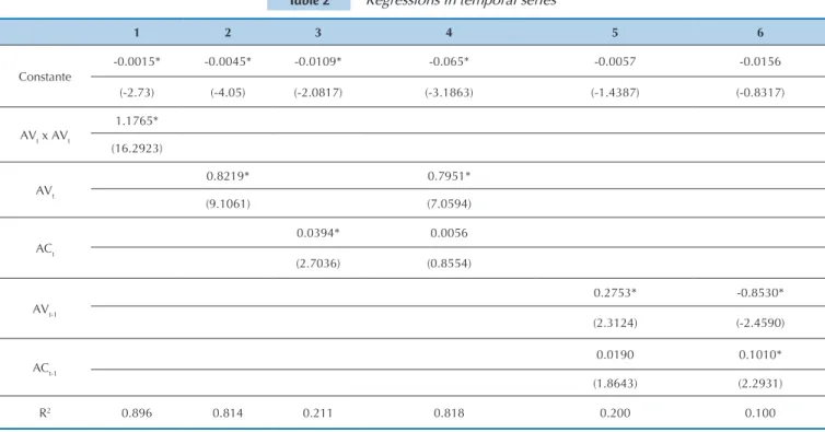
In Table 2 results of the OLS regressions, which seek to analyze the role of average variance and average cor-relation in explaining changes in market variance and in excess market return, are presented. For all the regres-sions t statistics from Newey-West were adopted with 4 lags. In column 1 the relationship between market va-riance and the product of its two components is presen-ted. The constant, despite being statistically significant, exhibits a value very close to zero. The product of the components explains practically all the contemporary variation in market variance, as demonstrated by the R2 of approximately 90%. In column 2 the relevance of the AV component in relation to changes in market varian-ce, is presented, reaching 81%, while column 3 refers to the average correlation, which captures 21% of these changes. An indication of greater relevance of the ave-rage variance component in the behavior of market va-riance can be noted here. In column 4 the two market variance components in the regression are included. To-gether, AV and AC explain approximately 82% of con-temporary market variance, and only AV turns out to be statistically significant. If compared with the result in column 2, it is perceived that the inclusion of AC in the model does not add practically any explanatory power. In column 5 a test of the predictive ability of AV and AC in the behavior of market variance is carried out, finding an R2_{of 20%; the same test carried out for US}

Figura 1.a Monthly market portfolio variance, Vm,

calculated as in Equation 13 and the product of average variance, AV – calculated as in Equation 14, and the average correlation, AC – average of the correlation to the pair of the return on assets each month. Sample period – July 2003 to July

2014.

(9)

monstrates that a worsening of investment conditions also depends on an increase in market variance. As a positive shock in AV indicates a reduction in excess ex-pected market return and an increase in exex-pected va-riance, this variable indicates a deterioration of future investment conditions, both in terms of expected re-turn as well as risk. A variable with these characteristics should command a risk premium. Assets that respond well when positive shocks in AV occur serve as a hedge in poor market conditions and, therefore, should have a lower expected return. According to Chen and Petko-va (2012), assets that respond well to positive shocks in AV are assets with high investments in research and development. This type of investment, due to its inno-vative character, offers alternatives for periods of crisis, meaning this asset/portfolio serves as a hedge. Conse-quently, its expected return will be lower (negative risk premium).

data presents an R2_{of 22% (Chen & Petkova, 2012).} Co-lumn 6 presents a predictive regression of excess market return in relation to average variance and to average correlation of market variance. The R2_{found was 10%,} that is, superior to that found in the same procedure for US data, which was 2% (Chen & Petkova, 2012). This degree of ability of the model to explain excess market return one period ahead, according to Chen and Petko-va (2012), “is comparable to other studies that analyze the predictability of monthly market return”.

It is interesting to note that AV exhibits, according to the results reported in Table 2, a negative relationship with market excess in the following period, and a posi-tive one with market variance in the following period. Campbell (1993) presents a description of how a sho-ck in a variable that represents a reduction in expec-ted market return indicates a worsening in conditions for investors. Chen (2003) extends this result and

de-Table 2 Regressions in temporal series

1 2 3 4 5 6

Constante

-0.0015* -0.0045* -0.0109* -0.065* -0.0057 -0.0156

(-2.73) (-4.05) (-2.0817) (-3.1863) (-1.4387) (-0.8317)

AV_t x AV_t

1.1765*

(16.2923)

AVt

0.8219* 0.7951*

(9.1061) (7.0594)

ACt

0.0394* 0.0056

(2.7036) (0.8554)

AV_t-1

0.2753* -0.8530*

(2.3124) (-2.4590)

ACt-1

0.0190 0.1010*

(1.8643) (2.2931)

R2 _0.896 _0.814 _0.211 _0.818 _0.200 _0.100

Regressions in temporal series: contemporary (columns (1) and (4)) and predictive (5) for market variance, Vm, and predictive (6) for excess market return, Rm. The explanatory variables are AV x AC, AV, and AC. t statistics from Newey-West with four lags are in brackets. The asterisk indicates significance of 5% or less. Source: Developed by the authors.

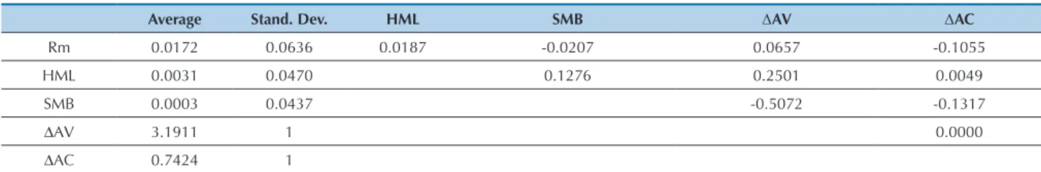
Table 3 below summarizes the average and the standard deviation of the factors used to capture the sensitivity (lo-ads) of portfolios sorted by company size and by idiosyn-cratic volatility. Subsequently, these loads will be used to explain the price of risk of each of these factors in relation

(10)

Table 3 Average and correlation of factors

Average Stand. Dev. HML SMB ΔAV ΔAC

Rm 0.0172 0.0636 0.0187 -0.0207 0.0657 -0.1055

HML 0.0031 0.0470 0.1276 0.2501 0.0049

SMB 0.0003 0.0437 -0.5072 -0.1317

ΔAV 3.1911 1 0.0000

ΔAC 0.7424 1

Presents the sample average, the standard deviation and the correlation for the Fama and French factors, Rm, HML, and SMB, and the innovations in average variance, AV, and in the average correlation, AC. The innovations in AV and AC derive from the orthogonalized and normalized VAR described in item 3.5.

Source: Developed by the authors.

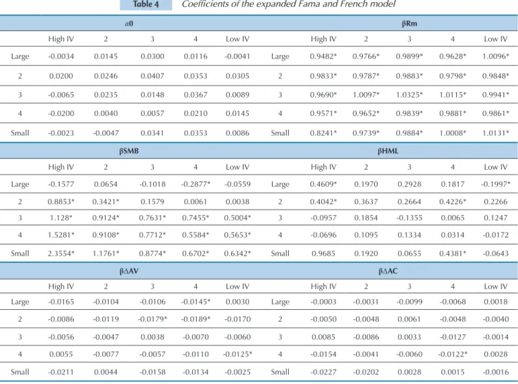
Table 4 presents the coefficients that indicate the sensitivity of each portfolio to the factors from the Fama and French (1996) model, increasing by the va-riation in average variance, ΔAV, and by the vava-riation in average correlation, ΔAC. The values indicate that the model adjusts well, and that the factors that are clear-ly more important for the Brazilian market are: excess market return, Rm; and the company size factor, SMB.

With regards to the average variance factor, assets that perform well in periods of market deterioration should have a positive load in relation to a variation in AV, since this variable predicts an increase in volatili-ty and a reduction in average market return (cf. Table 2). Inversely, assets with weak performance in perio-ds of crisis should exhibit a negative load in relation to a variation in AV. If the Brazilian data reproduced the US results, loads with changed signs would be ex-pected for portfolios with high and low idiosyncratic volatility, however, in contrast to the US market, this is not verified, according to the results find in this study. Chen and Petkova (2012) verify that, in the American economy, companies with high (low) IV exhibit a high (low) level of investment in research and development (R&D), which is considered as an indication of the pre-sence of real options. According to the literature, the value of a real option rises with an increase in volatility of the underlying asset. This fact would explain, for the US market, the characteristic of companies that have high (low) IV performing better (worse) in periods of crisis, and consequently, having positive (negative) sensitivity to the AV variation factor. In Brazil, almost all of the portfolios exhibited a negative load both in relation to AV variation as well as AC variation, with almost all also being statistically insignificant, despite these factors improving the explanatory power of the model. The conclusion which is drawn is that, for the Brazilian market, idiosyncratic volatility does not de-rive from sources that mitigate effects of a worsening in conditions for investors, i.e., it does not derive from R&D.

Another important point is that the ΔAV loads should rise from the portfolios with lower IV to those with higher IV, as predicted in Equation 6, which is also not verified in the Brazilian case.

The explanation for this difference between Brazil and the United States may be in the culture of

invest-ment in R&D. Trademarks and patents registration in Brazil is substantially lower than in the United States. The number of patents registered by each country was taken as a proxy for the volume of investment in R&D, according to data from the PCT Yearly Review (2014), from the World Intellectual Property Organization (WIPO), an agency of the UN. The total patent requests filed by the United States in 2013 were approximately 57,000, with 85% being from private companies. In the same period, Brazil filed approximately 620 patent re-quests, with only 50% of this total being of private ori-gin. Chen and Petkova (2012) cite this factor as one of the main ones for mitigating negative effects in periods of crisis. According to the authors, companies with a high level of R&D would serve as a hedge in periods of market deterioration, which would lead investors to accept paying a premium for them. This effect would cause a differentiation in the price of risk of these as-sets; their sensitive loads to the factors that predict a worsening in the market would be positive, that is, they would perform better than other companies in poor scenarios, leading to a negative price of risk, that is, a reduction in their expected return, since they would be seen as lower risk companies.

None of the above effects were identified in Brazil. The assets’ indicative sensitivity loads to a worsening in the market are practically all statistically null, as can be observed in Table 4. This would indicate that there would not exist assets with better or worse average per-formance in poor periods, in relation specifically to this risk factor. The average price of risk identified for this factor was significant – as can be seen in Table 5 – and positive, that is, the opposite of what was found for US data.

(11)

Table 4 Coefficients of the expanded Fama and French model

α0 βRm

High IV 2 3 4 Low IV High IV 2 3 4 Low IV

Large -0.0034 0.0145 0.0300 0.0116 -0.0041 Large 0.9482* 0.9766* 0.9899* 0.9628* 1.0096*

2 0.0200 0.0246 0.0407 0.0353 0.0305 2 0.9833* 0.9787* 0.9883* 0.9798* 0.9848*

3 -0.0065 0.0235 0.0148 0.0367 0.0089 3 0.9690* 1.0097* 1.0325* 1.0115* 0.9941*

4 -0.0200 0.0040 0.0057 0.0210 0.0145 4 0.9571* 0.9652* 0.9839* 0.9881* 0.9861*

Small -0.0023 -0.0047 0.0341 0.0353 0.0086 Small 0.8241* 0.9739* 0.9884* 1.0008* 1.0131*

βSMB βHML

Large -0.1577 0.0654 -0.1018 -0.2877* -0.0559 Large 0.4609* 0.1970 0.2928 0.1817 -0.1997*

2 0.8853* 0.3421* 0.1579 0.0061 0.0038 2 0.4042* 0.3637 0.2664 0.4226* 0.2266

3 1.128* 0.9124* 0.7631* 0.7455* 0.5004* 3 -0.0957 0.1854 -0.1355 0.0065 0.1247

4 1.5281* 0.9108* 0.7712* 0.5584* 0.5653* 4 -0.0696 0.1095 0.1334 0.0314 -0.0172

Small 2.3554* 1.1761* 0.8774* 0.6702* 0.6342* Small 0.9685 0.1920 0.0655 0.4381* -0.0643

βΔAV βΔAC

Large -0.0165 -0.0104 -0.0106 -0.0145* 0.0030 Large -0.0003 -0.0031 -0.0099 -0.0068 0.0018

2 -0.0086 -0.0119 -0.0179* -0.0189* -0.0170 2 -0.0050 -0.0048 0.0061 -0.0048 -0.0040

3 -0.0056 -0.0047 0.0038 -0.0070 -0.0060 3 0.0085 -0.0086 0.0033 -0.0127 -0.0014

4 0.0055 -0.0077 -0.0057 -0.0110 -0.0125* 4 -0.0154 -0.0041 -0.0060 -0.0122* 0.0028

Small -0.0211 0.0044 -0.0158 -0.0134 -0.0025 Small -0.0227 -0.0202 0.0028 0.0015 -0.0016

volatility. Thus, the greater exposure of this risk factor prices a higher expected return and vice versa – positive premium. The results obtained in this study record that

the hedge effect observed in the United States – gene-rated, according to Chen and Petkova (2012), primarily by investments in R&D – is not reproduced in Brazil.

Column 1 of Table 5 presents the prices of risk for the standard model. γ₀ is statistically signiicant and re-presents the pricing error in the model. Although it con-tinues to be diferent to zero in the other regressions, the components of the expanded model are not tradable portfolios, so nothing can be said about their signii-cance. When the factors regarding the market volatility components are inserted into the model, their explana-tory power increases. γ_ΔAV exhibits signiicance in all the experiments, indicating that the ΔAV component is pri-ced in excess return on the portfolios. Another interes-ting point is the relationship between ΔAV and ΔVm. As

This table presents the constant and the regression loads of 25 the portfolios sorted by size and idiosyncratic volatility (IV). The betas are calculated in the full sample.

The independent variables are the Fama and French factors with portfolios rebalanced monthly, plus the ΔAV and the ΔAC. The model is described in 3.5. The asterisk

indicates significance of 5% or greater, based on t statistic from Newey-West with four lags. The sample covers the period starting in January 2003 and finishing in July 2014.

(12)

Table 5 Regressions in temporal series

1 2 3 4 5 6

γ₀ -0.5889 -0.5934 -0.5800 -0.5888 -0.6090 -0.5896

(-6.2895) (-6.2255) (-5.9436) (-6.4878) (-6.5254) (-6.0769)

γ_Rm -0.3861 -0.3976 -0.3920 -0.3863 -0.3627 -0.3821

(-4.3756) (-4.2086) (-4.1925) (-4.5462) (-4.2123) (-4.1766)

γ_HML 0.0076 0.0092 0.0172 0.0076 0.0173 0.0178

(0.8847) (1.5544) (1.9211) (0.8445) (1.7730) (1.8601)

γ_SMB -0.0099 0.0143 0.0093 0.0099 0.0100 0.0096

(2.1967) (2.0275) (2.0580) (2.0346) (2.0838) (1.9248)

γ_ΔAV 0.8430 0.9482 0.9148 0.9546

(2.9175) (3.2703) (3.3694) (3.3611)

γ_ΔAC 0.1710 0.1324

(0.6486) (0.3941)

γ_ΔVm 0.1131 0.0678 0.0285

(0.7625) (0.6854) (0.2284)

R2 _0.21 _0.24 _0.26 _0.25 _0.25 _0.27

Fama and MacBeth regressions using excess returns on the 25 portfolios, sorted by size and idiosyncratic volatility. The betas are the independent regression variables

and were calculated for all of the sample. Rm, HTL, and SMB refer to the Fama and French factors, calculated with rebalanced portfolios month to month. ΔAV and ΔAC are the innovations in average variance and in average correlation, calculated as described in 3.5. ΔVm refers to the innovations in market variance and was calculated in a similar way to ΔAV and ΔAC. t statistics, in brackets, adjusted for error in the variables, as in Shanken (1992).

4.2 Complementary Analyses

In this paper, the Fama & French (1996) model with three factors is used, taking into consideration the intention of comparing the results found for the Brazilian data with those found for the US data, detai-led by Chen and Petkova (2012). Lately, the literature has recorded that five factor models have been shown to be better specified to describe returns (see Amihud, 2014). As we did not want to lose comparability, but, at the same time, sought to test robustness and present results in line with the more modern models, a brief reproduction of this paper’s main result was added, i.e., the risk premium for the average volatility (γ_ΔAV)

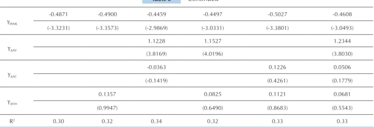
and average correlation (γ_ΔAC) components for portfo-lios ordered by idiosyncratic volatility, estimated based on the five factor model. Table 6 below reproduces the results presented in Table 5, and includes the two new factors, WML and IML, presented respectively by Ca-rhart (1997) and by Amihud (2014), in the analysis. These new factors were kindly supplied by the Nefin – FEA/USP team (n.d.). The results are robust and simi-lar to those presented for the three factor model. The γ_ΔAV exhibited is 1.12 – 0.94 in the three factor model – both statistically significant and positive. The γ_ΔAC is close to zero and not significant, as in the previous model.

Table 6 Regressions in temporal series – Five factor model

1 2 3 4 5 6

γ₀

-0.6045 -0.6002 -0.6652 -0.6579 -0.5700 -0.6334

(-6.2594) (-6.2717) (-6.7164) (-6.7826) (-5.3483) (-5.9926)

γ_Rm

-0.3684 -0.3727 -0.3064 -0.3135 -0.4029 -0.3380

(-4.0957) (-4.1767) (-3.4958) (-3.6498) (-3.9234) (-3.4814)

γ_HML

0.0087 0.0083 0.0060 0.0051 0.0077 0.0048

(1.1164) (1.0220) (0.7859) (0.6546) (0.9394) (0.6109)

γ_SMB

0.0096 0.0092 0.0080 0.0071 0.0085 0.0067

(2.1238) (1.9516) (1.7490) (1.5313) (1.8024) (1.4319)

γ_IML

0.0310 0.0316 0.0266 0.0271 0.0303 0.0264

(13)

Fama and MacBeth regressions using excess returns on the 25 portfolios, sorted by size and idiosyncratic volatility. The betas are the independent variables in the regression and were calculated for the whole sample. Rm, HML, SMB, and WML refer to the Fama and French factors. IML refers to the liquidity factor from Amihud

(2014). ΔAV and ΔAC are the innovations in average variance and in average correlation, calculated as described in 3.5. ΔVm refers to the innovations in market variance and was calculated in a similar way to ΔAV and ΔAC. t statistics, in brackets, adjusted for error in the variables, as in Shanken (1992).

As well as the analysis presented above, robustness tests were also carried out related to the quintiles and to the periods used in constructing the portfolios by size and IV. The test portfolios in the paper, as des-cribed previously, are composed of assets sorted by size and divided into five groups – 5 quintiles – and, subsequently, sorted by IV and divided again into five groups – another 5 quintiles – forming 25 studied por-tfolios. The nomenclature 5x5 will be adopted to refer to this composition. Thus, portfolios using 3x5 divi-sions would have three groups of shares sorted by size, followed by five groups of shares sorted by IV, forming 15 test portfolios in total. In order to evaluate robust-ness, different construction alternatives were elabora-ted for the test portfolios, such as 3x5, 3x6, 4x5, 4x6, and 5x6. Separate evaluations were also elaborated

in the first and in the second half of the sample. As a whole, the values found were shown to be robust. Al-tering the composition of the portfolios, the difference (spread) of average IV between the portfolios was also altered, thus modifying the sensitivity of the factors regarding volatility and correlation and, consequen-tly, influencing the magnitude of premium attached to these factors. However, the effect of the factors studied over the return on the portfolios was not altered, i.e., the average volatility component (γ_ΔAV) premium is po-sitive in all of the tests, while the average correlation (γ_ΔAC) component is statistically insignificant. These results align with the paper’s main results. In Table 7 some tests considered representative were reported; the rest, not reported, indicate quite similar values to those presented.

γ_WML

-0.4871 -0.4900 -0.4459 -0.4497 -0.5027 -0.4608

(-3.3231) (-3.3573) (-2.9869) (-3.0331) (-3.3801) (-3.0493)

γ_ΔAV

1.1228 1.1527 1.2344

(3.8169) (4.0196) (3.8030)

γ_ΔAC

-0.0363 0.1226 0.0506

(-0.1419) (0.4261) (0.1779)

γ_ΔVm

0.1357 0.0825 0.1121 0.0681

(0.9947) (0.6490) (0.8683) (0.5543)

R2 _0.30 _0.32 _0.34 _0.32 _0.33 _0.33

Table 6 Continued

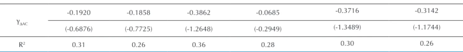
Table 7 Regressions in temporal series – Robustness tests

4x4 4x6 4x4 – 1st part 4x4 – 2nd part 4x6 – 1st part 4x6 – 2nd part

γ₀

-0.8396 -0.8245 -1.1015 -0.7090 -0.9898 -0.7251

(-8.382) (-9.6806) (-7.4717) (-7.5468) (-7.5335) (-7.7075)

γ_Rm

-0.1322 -0.1484 -0.0918 -0.0520 -0.2053 -0.0360

(-1.8181) (-2.7636) (-1.3394) (-1.2588) (-3.1626) (-0.9815)

γ_HML

0.0140 0.0099 0.0046 0.0022 -0.0060 0.0011

(1.6559) (1.1231) (0.3865) (0.2749) (-0.5323) (0.1511)

γ_SMB

0.0041 0.0054 0.0130 0.0090 0.0144 0.0079

(0.9247) (1.2481) (1.6671) (1.7612) (1.8569) (1.5496)

γ_ΔAV

0.5924 0.6278 0.4147 0.2562 0.7330 0.2000

(14)

5 CONCLUSIONS

In this study we used the fact that an asset’s idio-syncratic volatility – defined as the standard deviation of residuals in the Fama and French (1996) model – is directly affected by the absence of an explanatory factor in the model, in direct proportion to the sensitivity of the asset to the absent factor. Thus, idiosyncratic volati-lity can be seen as a proxy for a risk factor, in accordan-ce with Chen and Petkova (2012).

Following, therefore, the intuition of Ang et al. (2006) that market aggregate volatility is priced, even though it exhibits contradictory behavior, and of Chen and Petkova (2012), who, in order to explain this con-tradiction, propose to break aggregate volatility up into average variance and average correlation, it was analyzed whether idiosyncratic volatility is priced in the Brazilian market.

It was identified that the average variance compo-nent predicts a reduction in excess market return and an increase in variance, thus being a sign of deterio-ration in investment conditions. Average correlation exhibits ambiguous behavior, predicting an increase in excess return and an increase in variance. These results are consistent with the international literature. Thus, the decomposition of volatility into the two components

allows that average variance can better price the effects of a worsening or improvement in the investment envi-ronment, without the disturbance generated by the cor-relation component. These results are also identical to those found for US data, indicating that in Brazil, like in the United States, the average variance component should command a risk premium in relation to portfo-lios sorted by size and IV.

It occurs that, for US data, the risk premium com-manded by average variance is significant and negative. The main explanation indicated by Chen and Petkova (2012) for a negative premium is the high level of in-vestment in research and development by companies with a high level of IV. Portfolios composed of these companies would act as a hedge against deterioration of the environment and, thus, would have lower returns expectations. As the volume of investment of resear-ch and development recorded in Brazil is significantly reduced, if compared with that recorded in the United States, the expected result was that the Brazilian pre-mium was positive. In fact, this occurs, and the risk premium commanded by exposure to average variance, according to the results found, is statistically significant and positive.

Almeida, C. I., Gomes, R., Leite A. L., Simonsen, A., & Vicente, J.

V. (2009). Does Curvature Enhance Forecasting? International

Journal of Theoretical and Applied Finance, 12(08), 1171-1196. Amihud, Y. (2014). The Pricing of the Illiquidity Factor's Systematic

Risk. Working Paper, New York University, Stern School of

Business. Available at http://ssrn.com/abstract=2411856 or http:// dx.doi.org/10.2139/ssrn.2411856

Ang, A., Hodrick, R. J., Xing, Y., & Zhang, X. (2006). The

Cross-Section of Volatility and Expected Returns. The Journal of Finance,

61(1), 259-299.

Avramov, D., Chordia, T., Jostova G., & Philipov, A. (2013). Anomalies

and Financial Distress. Journal of Financial Economics, 108(1),

139-159.

Bonomo, M. & Agnol, I. D. (2003). Retornos Anormais e Estratégias

Contrárias. Revista Brasileira de Finanças, 1(2), 165-215.

Campbell, J. Y. (1993), Intertemporal Asset Pricing Without

Consumption Data. National Bureau of Economic Research,

Working Paper No. 3989.

Campbell, J. (1996). Understanding Risk and Return. Journal of

Political Economy. 104(2), 298-345.

Carhart, M. M. (1997). On persistence in mutual fund performance.

The Journal of Finance. 52(1), 57-82.

Chen, J. (2003). Intertemporal CAPM and the Cross-section of Stock

Returns. Working Paper, University of California, Davis.

Chen, Z., & Petkova, R. (2012). Does Idiosyncratic Volatility Proxy for

Risk Exposure?. Review of Financial Studies, 25(9), 2745-2787.

Costa Jr, N. C. A., & Neves, M. B. E. (2000). Variáveis Fundamentalistas e Retorno das Ações. In N. C. A. da Costa Jr., R. P. C. Leal, & E.

F. Lemgruber. Mercados de Capitais: Análise Empírica no Brasil.

Atlas, São Paulo.

Diebold, F. X., & Li, C. (2006). Forecasting the term structure of

government bond yields. Journal of Econometrics, 130(2), 337-364.

Driessen, J., Maenhout, P., & Vilkov, G. (2009). The Price of

Correlation Risk: Evidence from Equity Options. The Journal of

Finance, 64(3), 1377-1406.

Fama, E. F. & French, K. (1996, march). Multifactor Explanations of

References

Fama and MacBeth regressions using excess returns on different portfolios sorted by size and idiosyncratic volatility. The betas are the independent variables in the regression and were calculated for the whole sample in columns 4x4 and 4x6. The rest, in accordance with that indicated in the table – 1st_{and 2}nd_{parts of the sample.}

Rm, HML, and SMB refer to the traditional Fama and French factors. ΔAV and ΔAC are the innovations in average variance and average correlation, calculated as described in 3.5. t statistics, in brackets, adjusted for error in the variables, as in Shanken (1992).

Table 7 Continued

γ_ΔAC

-0.1920 -0.1858 -0.3862 -0.0685 -0.3716 -0.3142

(-0.6876) (-0.7725) (-1.2648) (-0.2949) (-1.3489) (-1.1744)

(15)

Correspondence Address:

André Luís Leite

Departamento de Administração, Pontifícia Universidade Católica do Rio de Janeiro Rua Marquês de São Vicente, 225 – CEP: 22451-900

Gávea – Rio de Janeiro – RJ Email: alleite@phd.iag.puc-rio.br

Asset Pricing Anomalies. The Journal of Finance, 51(1), 55-84.

French, K., Schwert W., & Stambaugh, R. (1987). Expected Stock

Returns and Volatility. Journal of Financial Economics, 19(1), 3-29.

Jensen M. C., Black, F., & Scholes, M. (1972). The Capital Asset Pricing

Model: Some Empirical Tests. Studies in the Theory of Capital

Markets. New York: Praeger Publishers, 79-121.

Lintner, J. (1965). The valuation of risk assets and the selection of risky

investments in stock portfolios and capital budgets. Review of

Economics and Statistics, 47(1), 13-37.

Lo, A.W., & MacKinlay, A. C. (2002). A non-random walk down Wall

Street. Princeton University Press.

Lucena, P., & Figueiredo, A. C., P. (2008). Anomalias no Mercado de Ações Brasileiro: uma Modificação no Modelo de Fama e French.

RAC-Eletrônica, Curitiba, 2(3), 509-530.

MacKinlay, A. C. (1995). Multifactor Models Do Not Explain

Deviations From The CAPM. Journal of Financial Economics,

38(1), 3-28.

MacKinlay, A. C., & Pastor, L. (2000). Asset Pricing Models:

Implications for Expected Returns and Portfolio Selection. Review

of Financial Studies, 13(4), 883-916.

Markowitz, H. M. (1952). Portfolio Selection. The Journal of Finance,

7(1), 77-91.

Mendonça, F. P., Klotzle, M. C., Pinto, A. C. F., & Montezano, R. (2012). The Relationship between Idiosyncratic Risk and Returns

in the Brazilian Stock Market. Revista Contabilidade & Finanças,

23(60), 246-257.

Merton, R. (1980). On Estimating the Expected Return on the Market:

An Exploratory Investigation. Journal of Financial Economics, 8(4),

323-361.

Merton, R. (1987). A Simple Model of Capital Market Equilibrium with

Incomplete Information. The Journal of Finance, 42(3), 483-510.

Mossin, J. (1966). Equilibrium in a Capital Asset Market. Econometrica,

34(4), 768-783.

Nefin – FEA/USP (n.d.). Brazillian Center for Research in Financial Economics. Núcleo de Estudos em Economia Financeira, da Faculdade de Economia, Administração e Contabilidade, da Universidade de São Paulo. Available at http://nefin.com.br

PCT Yearly Review (2014). World Intellectual Property Organization – WIPO. Disponível em www.wipo.int

Rayes, A. C. R. W., Araújo, G. S., & Barbedo, C. H. S. (2012). O modelo de 3 Fatores de Fama e French ainda explica os retornos no

mercado acionário brasileiro?. Revista Alcance – Eletrônica, 19(1),

52-61.

Ross, S. A. (1977). The Capital Asset Pricing Model (CAPM), Short-sale Restrictions and Related Issues. Journal of Finance, 32(1), 177-183.

Shanken, J. (1992). On the Estimation of Beta-pricing Models. Review

of Financial Studies, 5(1), 1-34.

Sharpe, W. F. (1964). Capital asset prices: A theory of market

equilibrium under conditions of risk. The Journal of Finance,

19(3), 425-442.

Svensson, L. (1994). Monetary Policy with Flexible Exchange Rates and

Forward Interest Rates as Indicators. Banque de France, Cahiers