Smart metering consumer behavior study in the Republic of Ireland: Further analyses on the consumers’ electricity consumptions and usage perceptions

(1)

A Work Project, presented as part of the requirements for the Award of a Masters Degree in Management from the NOVA – School of Business and Economics.

Smart Metering Consumer Behavior Study in the Republic of Ireland: Further Analyses on the Consumers’ Electricity Consumptions and Usage Perceptions

Helena Magda Agostinho Dias Number: 670

A Project carried out on the Management course, under the supervision of: Professor Luís Catela Nunes

(2)

2 Smart Metering Consumer Behavior Study in the Republic of Ireland: Further

Analyses on the Consumers’ Electricity Consumptions and Usage Perceptions

Abstract

With the disclosure of the conclusions of the Republic of Ireland’s Smart Metering Trials, this report intends to summarize the experience and the Consumer Behavior results. I also complement the Irish report by examining the effect of demographic and attitudinal variables in the change of electricity consumption during the trial and by studying the accuracy of the participants’ perception of the change in their consumptions and bills during the experience. The main conclusion is that the participants were not able to take full advantage of the potentiality of the Time-of-Use tariffs to reduce bills and did not have a clear perception of their consumptions and spending, which may have prevented them of achieving better results.

(3)

3

1. Introduction

Saving energy is essential for the world’s well-being as it creates economic and environmental benefits. Nonetheless, it constitutes a great challenge as the majority of the population does not act to reduce their energy consumptions or are clueless about how to do it1. Recognizing that, some countries are already implementing smart metering projects. A smart meter of electricity replaces the old meters, allowing real time readings instead of estimates and to read the meter remotely. They offer, as well, the possibility of applying time-of-use (ToU) tariffs, with rates that vary according to the period of the day. This type of project enables higher energy and bill savings, as the consumers have access to their real time consumptions and can also take advantage of the ToU tariffs. The electrical companies can also gain insights on consumers and meet their preferences and accomplish production and operational savings. Moreover, the energy savings also succeed on creating environmental benefits.

In 2011, this novelty was introduced in Portugal with EDP’s InovCity project, still being conducted in Évora. However, in the Republic of Ireland the experience is already concluded by the Commission for Energy Regulation which is presently making its final decision on proceeding with a full roll-out across the country. This report aims firstly to resume and describe the Irish Smart Metering trials and its results on residential consumers. Secondly, to understand what kind of factors (e.g. demographic, attitudes) affect how the residential customers' electricity consumption patterns react to changes in electricity prices and to different stimuli. Finally, to analyze how correct are the perceptions of the trial’s participants of changes in their consumptions and bills. This report supplements the results obtained by the Irish experience, contributing with

1

As discovered by the North-American study “Public perceptions of energy consumption”, by PNAS (Proceedings of the National Academy of Sciences of USA), in 2010.

(5)

5

statistical studies that can be used as reference for comparisons by other Smart metering projects, like the Portuguese one2, when studying their own results.

2. Smart metering experience in the Republic of Ireland

2.1. Description of the experience

In 2007 the Commission for Energy Regulation (CER), the “independent body responsible for overseeing the liberalization of Ireland's energy sector”3

, started to structure a Smart metering project with the objective of running smart metering trials across a sample of residential households and small and medium enterprises, in order to evaluate the costs and benefits of the experience and the information required for a full roll-out across the country. For the full year of 2010 the trials were conducted and in May of 2011 the finding reports with the experience’s conclusions were published on CER’s website, allowing for public consultation. The final results were considered positive so a full roll-out is now a solid premise. The trials produced three different types of analyses: Cost-benefit, Technological and Customer Behavior. As the focus of this report is the Residential Customer Behavior analysis, a further explanation on the process undertaken and the results obtained by CER is provided on the following pages.

The Customer Behavior experience was divided in four periods. First, the Pre-benchmark period from March of 2008 to June of 2009 in which the components of the trial were designed and the participants contacted by letter, with the recruitment of consumers from different demographic, behavioral and usage profiles to assure representivity. The smart meters were also installed in the participants’ houses during this phase. Secondly, from the 1st of July to the 31st of December of 2009, the Benchmark phase took place, with the collection of consumption data, the performance

2_{A reunion I attended with a Marketing Manager in EDP, in which I described the Irish experience,}

confirmed EDP’s great interest in this study.

(6)

6

of pre-trial surveys to understand the behavior changing interest of the participants and the allocation of participants between the control group and the various test groups. Then, from January to December of 2010, the Test period occurred. Lastly, in the Post-trial period, in January and February of 2011, the participants returned to the pre-Post-trial tariff and billing and post-trial consumer behavior surveys were conducted through Computer Assisted Telephone Interviewing (CATI).

The post-trial survey consisted of approximately 200 questions, mostly structured multiple-choice ones. It comprised some demographic and attitudinal questions, which were responded both by the control and test group, and questions related to the smart metering experience only answered by the test group. The latter set of questions, all relatively to the experience, were about changes accomplished, difficulties experienced, perception of changes in usage and bill achieved, factors that encouraged to reduce consumption, the tariffs and the demand side management (DSM) stimuli.

This experience had the main goals of understanding if the combination of the smart meters with Time of Use (ToU) tariffs and DSM stimuli was effective at reducing the consumption of electricity and also if there was a Tipping Point, which is the point in that the price of electricity would significantly change usage.

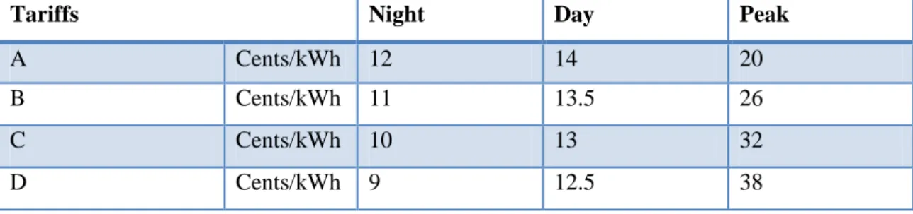
One of the components of the trial was the ToU tariffs, which are tariffs with different electricity prices according to the time of the day. The participants of the test group were distributed between four main groups of tariffs (A, B, C and D) and the “Weekend group”. There were three different periods with different rates (in cents/kWh): the Night period from 11pm to 7.59am, with lower prices; the Day period from 8am to 4.59pm and from 7pm to 10.59pm with intermediate prices; and the Peak period from 5pm to 6.59pm, with higher prices. The peak rates were not considered during weekend and

(7)

7

federal holidays, being replaced and tariffed as day period. Tariffs A, B, C and D had different prices according to the period of the day that can be observed in Table 1.

Tariffs Night Day Peak

A Cents/kWh 12 14 20

B Cents/kWh 11 13.5 26

C Cents/kWh 10 13 32

D Cents/kWh 9 12.5 38

Table 1- ToU tariffs

It is possible to detect that Tariff A had the most approximated prices, with the lower peak price of the four groups but with the higher night rate, whereas Tariff D had the most dispersed ones, with the higher peak price and lower night price. As mentioned, there was also a Weekend group, in which some participants of the test group were allocated. During the week this group had high day (14cents/kWh) and peak rates (38cents/kWh) and low night rates (10cents/kWh), however during the weekends the price was always a low 10cents/kWh independently of the period. The control group did not experienced ToU tariffs, being billed with the previous fixed tariff of 14.1cents/kWh of their regular electricity supplier, Electric Ireland4.

Another constituent of this smart metering experience were the demand side management5 stimuli. The Irish trial counted with four different stimuli, in which the test group participants were spread. Stimulus 1 (S1) was a bi-monthly bill (every other month) combined with an Energy Usage Statement. The Energy Usage Statement (EUS) was a document attached to the bill that contained additional detail about the electricity consumption, as information on average weekly costs and usage, on how the consumers were doing compared to the last bill and to the other participants of their

4

At the time the participants were recruited and allocated to the test and control groups, Electric Ireland represented the entire electricity market. During the trial, some competition appeared with a small percentage of participants, both from the test and control groups, quitting the experience.

5

Demand side management is the use of diverse methods, commonly financial incentives and education, to change the consumer demand for energy.

(8)

8

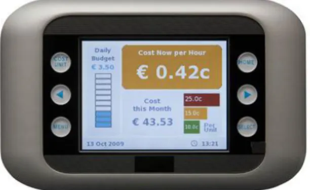
group and it also enclosed tips to reduce consumption and move it from peak hours. Stimulus 2 (S2) was a monthly bill plus the EUS. Stimulus 3 (S3) was a bi-monthly bill, the EUS and an electricity monitor. The monitor (Figure 1) was an in-home display to help consumers be more aware of their energy usage. It provided information on how much energy the participants were using at any time and how much it was costing them and also allowed them to set a daily budget of the maximum they wanted to spend, showing how much they were spending against the budget.

Figure 1- Electricity Monitor

Stimulus 4 (S4) was a bi-monthly bill, the EUS and an Overall Load Reduction (OLR) Incentive. This incentive involved setting a target of energy reduction: the usage verified in that month in the previous year, less 10%. The participants were updated in the bi-monthly bill on their progress and in the end, if the participants had been successful (during all months), they would receive a 20€ credit reward.

All the test participants received extra information, with the prices and times of their tariff group under the form of fridge magnets and stickers. The control group participants did not receive any stimuli or extra-information and were asked to continue to use energy as they would normally do.

The population was stratified to assure representivity across all groups in factors as socio-demographic profile, energy usage, household size and interest in changing the

(9)

9

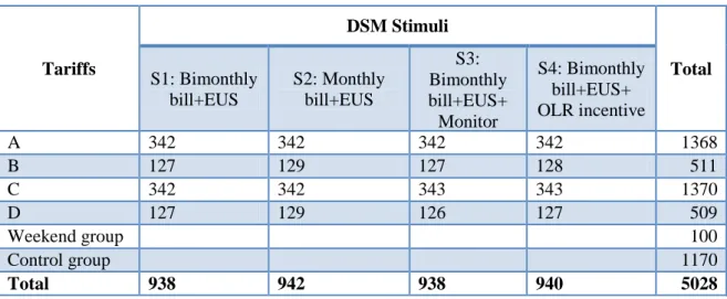
behavior. Then, each household was randomly allocated in one of the different groups. Table 2 reproduces the distribution of the participants.

Tariffs DSM Stimuli Total S1: Bimonthly bill+EUS S2: Monthly bill+EUS S3: Bimonthly bill+EUS+ Monitor S4: Bimonthly bill+EUS+ OLR incentive A 342 342 342 342 1368 B 127 129 127 128 511 C 342 342 343 343 1370 D 127 129 126 127 509 Weekend group 100 Control group 1170 Total 938 942 938 940 5028

Table 2- Allocation of participants

2.2 Main results

The analyses of consumptions and post-trial surveys had the objective of verifying if and which groups had been able to reduce the overall electricity consumption and move the usage away from the peak time to other periods. Two different types of results6 were included in the Consumer Behavior Findings Report published by CER, the ones related to the actual consumption’ changes accomplished by the different groups of tariffs and stimuli and the results obtained from the post-trial surveys.

Results: tariffs and stimuli

 The tariffs with the stimuli obtained a 2.5% overall reduction and a 8.8% reduction at peak hours on the test group consumptions relatively to the control group.

 The Weekend Tariff obtained the bigger reductions both overall (3.7%) and at peak time (11.6%). Apart from the Weekend Tariff, Tariff B achieved the larger overall reduction (3.4%) and Tariff D the bigger at peak hours (10.9%).

(10)

10

 Stimulus 3 stood out as more effective at peak (11.3%). Stimulus 1 was not as effective at decreasing consumption as the other stimuli.

 Of the tariff groups tested, no single one in combination with DSM stimuli stands out as being more effective than the others and the same happens for all the stimuli in combination with the tariffs, at a 90% statistical confidence level.

 CER was not able to find a Tipping Point, in which the price premium causes a significant reduction in usage7. This was measured by observing that despite the average daily peak usage being lower for the tariff groups with a higher peak rate, there was a weak relationship between price (the tested Tariffs) and usage reduction.  The use reduced from peak hours was mostly transferred to the period immediately

post-peak and some to the night period.

Results: Consumer behavior post-trial survey

 Most participants mistakenly estimated that the percentage in the bill reduction would be equal to the percentage in usage decrease, as they forgot the effect of the ToU tariffs: the change in bill depends not only on the change in usage in different periods but also on the changes in the corresponding prices.

 The households with higher socio-economic levels achieved higher reductions but they also had higher levels of consumption to begin with.

 Households with more children, with and under 15 years old, reached higher reductions. CER concluded that children motivate change and energy reduction.  25% of the participants found it hard to move from peak hours and 14% had trouble

moving to the night period due to questions of noise, security and inconvenience.  54% believed they became more aware of energy spending but only 22% said that

they know how to reduce usage after the trial.

(11)

11

 The informative magnets and stickers were found effective by the majority.

 The electricity monitor was found useful and easy to use; however most participants did not know or did not try to change the settings.

 The consumers found effective the Energy Usage Statement and bills.

 Only half remembered the Overall Load Reduction Incentive and 25% were successful. But it received good efficacy scores in the survey, so CER believes that the problem was not its efficacy but that participants did not remember it.

 Most participants claimed that they accomplished big changes with the trial.

3. Statistical analyses’ guideline

The Consumer Behavior analysis conducted by CER, despite extensive, did not entail all the studies that were possible to perform. My report aims to increase and complement to some extent CER’s study with two core analysis. The first one’s purpose is to verify if demographic, attitudinal factors and stimuli, by themselves and combined with tariffs, are associated with the reduction in overall and peak usage. However, contrarily to CER’s study I proceeded to include all the variables, except the stimuli, in a multiple regression analysis, instead of investigating variable by variable, as together they are able to reflect the effects of their interactions. Nonetheless, I analyzed separately the stimuli and their respective combinations with the peak price as CER distributed demographically the participants in a representative way by all stimuli. The second analysis’ drive is to deeply understand how accurate were the participants’ perceptions of the change in the consumptions and the bills with the trial. All investigations were developed with the data provided by CER: the consumptions of the Trial’s participants and the answers to the Consumer Behavior surveys.

(12)

12

For the consumption, only data from the last six months of 2009 (pre-trial) and for the full year of 2010 (during the trial) were provided. For the first months of 2010 the experience was a stirring new advent to the test group participants, specially, as they started to receive DSM stimuli. Only after the first months of excitement did the consumers started to act more closely to what is expected to be the behavior in a full roll-out, after the first impact. In order to facilitate the comparison of data and to eliminate the effect of the initial enthusiasm, I used only the last six months of 2010’s data. For each participant, it was calculated the average consumption per period, day, night, peak and overall (the sum of all), both for 2009 and 2010. Then, for each period, the value of 2009 was subtracted from 2010 and it was possible to understand if there had been savings (negative value) or not.

To avoid being too extensive, this report concentrates on the differences of consumption at peak and overall and not on the night and day usages. The two components I chose to focus are the most important: overall consumption includes all the periods and reflects the participant’s ultimate results and peak consumption reduction was one of the main goals of the experience. Likewise, the weekend test group is not comprised in this report for its weak expression in the experience (only 100 participants) and because it did not include DSM stimuli. Only the four main tariffs of the test group (A, B, C, and D) are compared to the control group. The following analyses were performed using SPSS (Statistical Package for Social Sciences) and Excel.

4. Analysis of demographic and attitudinal factors

4.1. Explanation of variables and Factor analysis

For the first analyses only the demographical and the answers to the attitudinal questions (provided both by the test and control group) from the Consumer Behavior

(13)

13

Survey were used, for comparison effects. The survey’s demographic questions were about Age, Employment status, Social class, Total number of people in the household, Number of children in the household, Rent or own the house, Number of people spending at least 5-6 hours in the house during the day. The Age question was excluded from these analyses as it had too many missing responses since the majority of the participants chose not to answer it. The Employment status was grouped in three categories: employed, unemployed and retired. The Social class was divided in five classes, AB, C1, C2, DE, F, with AB corresponding to the highest and F to the lowest8.

Component Matrix

Component

1 2 3

Q1: I want to reduce usage if it helps the environment. .620 .357 -.187 Q2: I can reduce the bill by changing my usage. .527 .413 -.279 Q3: I want to reduce usage if it decreases the bill. .600 .405 -.285 Q4: I have made a lot of effort to reduce consumption. .532 .087 .664 Q5: I changed the way I live to reduce consumption. .540 .193 .603 Q6: I want to do more to reduce consumption. .535 .385 -.189 Q7: I know what to do to decrease consumption. .378 .135 .305

Q8: I cannot control my consumption. -.393 .469 .056

Q9: It is inconvenient to reduce usage. -.497 .463 .097

Q10: I cannot get the people I live with to reduce usage. -.258 .547 -.221 Q11: I do not have time to reduce consumption. -.438 .570 .011 Q12: I do not want to be told how much energy I consume. -.379 .378 .282 Q13: Decrease usage will not make any difference to the bill. -.452 .312 .296 Extraction Method: Principal Component Analysis.

a. 3 components extracted.

Table 3- Factor analysis

The attitudinal questions included in this analysis are about the participants’ general attitude towards energy, their efforts and difficulties felt during the trial to reduce electrical usage. For each statement, the respondents had to rate from 1 to 5, with 1

8_{The Social grades were attributed according to the NRS social grade system, with AB being the upper}

middle and the middle class; C1 corresponding to the lower middle class; C2 to the skilled working class; DE to the working class and F to the farmers.

(14)

14

being strongly disagree and 5 strongly agree. There was also the option 6, “don’t know”, transformed in a missing response for the purpose of this report’s study.

I conducted a Factor Analysis with all of these variables, in order to detect a smaller number of factors that may explain the majority of their variance. A Kaiser-Meyer-Olkin analysis, a measure of sample adequacy that tests whether the partial correlations among variables are small, provided a value of 0.758 (>0.5), indicating that a factor analysis was appropriate. With a Barlett’s test of Sphericity the null hypothesis that the variables were uncorrelated in the population was also rejected. The Principal Component Analysis9, detected three factors (Table 3): variables Q1 and Q3 are highly correlated with Factor 1, which are related with the Motivations to reduce electricity usage; Q8, Q9, Q10 and Q11 are more correlated with Factor 2, Difficulties in reducing usage; and Q4 and Q5 with Factor 3, Pro-activity to reduce consumption. These three factors, instead of every single variable, are used in the regression analyses which results are presented in the following sub-section of this report.

4.2. Impact of DSM stimuli on attitudes

To understand if the three attitudinal factors were affected by the DSM stimuli, some regressions were performed in which the dependent variables were each of the factors. Multicollinearity happens when two or more variables are perfectly correlated and results in the dummy variable trap10. To avoid it one of the dummy variables for each set of categories was left out of the analysis, being the base dummy variable. This way, whenever one of the dummies was taken out, the others of the same category would provide their result in relation to the excluded one.

9_{Criteria: retaining components with an Eigenvalue higher than 1.}

10_{The dummy variable trap occurs when dummies for all categories are included in the analysis and their}

sum is equal to 1 for all observations, being perfectly correlated with the constant variable. If the constant variable is also included in the model, it will result in multicollinearity.

(15)

15

Following the same method of CER’s report, I considered the variables significant at a 90% level.

Coefficients Dependent variable FACTOR 1:

Motivations FACTOR 2: Difficulties FACTOR 3: Pro-activity Model Unstandardized Coefficients Sig. Unstandardized Coefficients Sig. Unstandardized Coefficients Sig. B Std. Error B Std. Error B Std. Error 1 (Constant) .076 .042 .070 .036 .042 .386 .008 .042 .847 S1:Bimonthlybill -.013 .060 .828 -.013 .060 .829 .005 .060 .935 S3:Monitor -.039 .060 .521 -.066 .060 .273 .088 .060 .143 S4:Incentive -.116 .059 .050 .019 .059 .745 .028 .059 .634 Control group -.197 .058 .001 -.114 .058 .048 -.142 .058 .014 Table 4- Regression analyses for factors

In Table 4, the excluded dummy was Stimulus 2 (EUS + monthly bill), so the results for the other variables are always in comparison to this one. When the dependent variable is Factor 1, taking into account the significance of the estimated coefficients, we conclude that participants with Stimulus 4 (EUS + bi-monthly bill + incentive) and especially those in the control group (more significant) feel less motivated to reduce usage, during the course of the experience, relatively the other groups (Stimuli 1, 2 and 3). For Factor 2 only the control group is significant, claiming to feel few difficulties in reducing usage, possibly reflecting a lack of awareness of the households in this group. When the dependent variable is Factor 3 the control group participants felt less pro-active to reduce consumption, as expected.

4.3. Regression analyses

I conducted regression analyses, resulting in Table 5, to understand the effect of multiple variables on the change in consumption achieved during the trial. In the first group of columns the dependent variable is the change, from 2009 to 2010, in the

(16)

16

average consumption during peak periods measured in kWh, and in the second is the change in overall consumption. The independent variables considered were the demographic variables (Employment status, Social class, Total number of people in the household, Number of children in the household, Rent or own the house, Number of people spending at least 5-6 hours in the house during the day), the three attitudinal factors identified by the factor analysis (denoted by Factor1, Factor2, and Factor3), the stimuli (studied separately from the other independent variables) and the price at peak and its interaction with each of the previous variables. The peak price, denoted in the tables as “delta_price_peak”, was calculated as the difference between the price per kWh without the trial (14.1 cents) and the tariff’s price. For instance, for the control group the “delta_price_peak” is zero, as the control group’s price remains the same 14.1 cents. Besides the control group, tariff A is the one with the lower peak price and tariff D the higher, since the peak prices increase as the tariff’s grade (A to D) advances. It is important to keep in mind that whenever one of the demographic or attitudinal variables appears alone it is considering all the participants (the control and test group) and measuring the change in consumption for those characteristics globally, not capturing how the trial (peak price and stimuli) affects them. Only the variables interacting with the peak price measure the effect of the peak price across the different features.

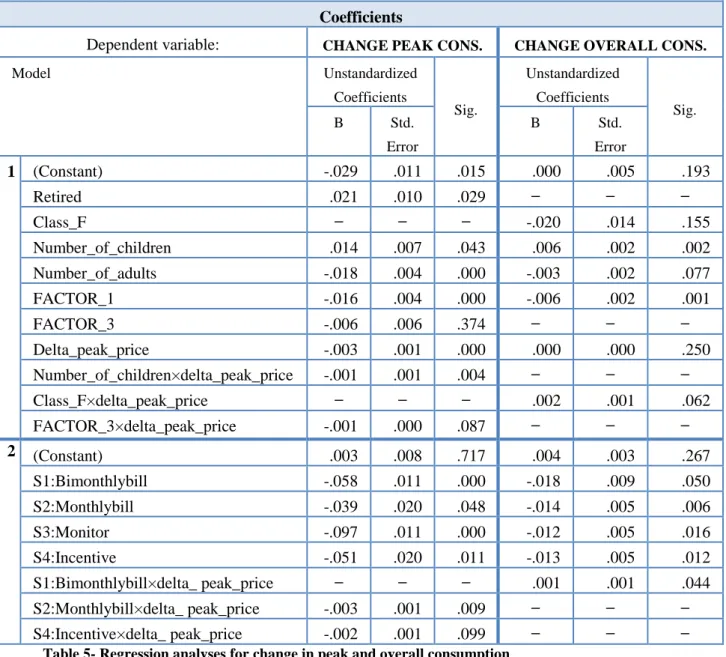
Since in the model including all explanatory variables many were non-significant, it was performed an analysis that excluded one by one the non-significant ones, starting by the interactions, until only significant variables remained, with the caution of not leaving out any of the single variables that were included in one of the significant interactions. The estimation results of the final models, applying this method, are summarized in the following table:

(17)

17 Coefficients

Dependent variable: CHANGE PEAK CONS. CHANGE OVERALL CONS.

Model Unstandardized Coefficients Sig. Unstandardized Coefficients Sig. B Std. Error B Std. Error 1 (Constant) -.029 .011 .015 .000 .005 .193 Retired .021 .010 .029 Class_F -.020 .014 .155 Number_of_children .014 .007 .043 .006 .002 .002 Number_of_adults -.018 .004 .000 -.003 .002 .077 FACTOR_1 -.016 .004 .000 -.006 .002 .001 FACTOR_3 -.006 .006 .374 Delta_peak_price -.003 .001 .000 .000 .000 .250 Number_of_children×delta_peak_price -.001 .001 .004 Class_F×delta_peak_price .002 .001 .062 FACTOR_3×delta_peak_price -.001 .000 .087 2 (Constant) .003 .008 .717 .004 .003 .267 S1:Bimonthlybill -.058 .011 .000 -.018 .009 .050 S2:Monthlybill -.039 .020 .048 -.014 .005 .006 S3:Monitor -.097 .011 .000 -.012 .005 .016 S4:Incentive -.051 .020 .011 -.013 .005 .012 S1:Bimonthlybill×delta_ peak_price .001 .001 .044 S2:Monthlybill×delta_ peak_price -.003 .001 .009 S4:Incentive×delta_ peak_price -.002 .001 .099

Table 5- Regression analyses for change in peak and overall consumption

From Table 5 it is possible to observe that:

 The variables presented alone were globally (both for the test and control group) significant for a change in peak or overall consumption, but they do not show how the trial affected them, as explained above. These variables are the retired participants compared to the employed (the left out dummy variable), social class F (compared to class C1), the number of children and of adults in the household, Factor 1 (motivation to reduce usage) and Factor 3 (pro-activity to reduce consumption).

(18)

18

 The peak price (“delta_peak_price”) while not significant for the change in overall consumption provided the following result: the participants with higher peak price were more able to achieve savings at peak during the trial.

 The groups reacting more to a change in peak price are the households with more children and the participants that agreed more with Factor 3, being more pro-active to reduce consumption. Both groups attained savings at the peak period.

 Participants from class F that have higher peak prices increased their overall electricity usage.

 All the stimuli, comparing to the control group (i.e. without any DSM stimulus), contributed to a decrease in peak and overall usage during the trial, paralleled to 2009. For peak consumption, Stimulus 3 (EUS, bi-monthly bill and monitor) stood out as the more effective reducing usage.

 As the peak price increases, Stimulus 2 (EUS and monthly bill) contributes for a decrease in peak consumption, so peak consumption reacts more to higher peak prices only when there is more direct feedback through more frequent billing (not with the monitor). Stimulus 4 (EUS, bi-monthly bill and incentive to reach a target of usage savings) also contributes for a reduction in consumption, but is almost non-significant.

 For overall usage, participants with Stimulus 1 (EUS and a bi-monthly bill) with higher peak prices appear to produce negative results, increasing consumption.  The remaining variables not included in the table were not significant, meaning that

the fact that the participants were in these categories did not interfere with the change of peak or overall consumption during the trial.

(19)

19 4.4. Analysis of results

Some of the above results may seem curious or to be contradictory to CER’s conclusions.

Contribution of children to savings

While children, observed globally, contributed to less peak and overall savings, we observed that more children in a household combined with higher peak prices decrease peak consumption. One possible explanation is that children of the test group were exposed to stimuli and felt the urge to spend less or influence their family to do so during the periods with higher electricity rates.

Social classes

Contrary to CER’s conclusions, it seems that higher social classes were not significant for the consumption’s changes during the trial. Only the lower provided results. This could have happened because CER analyzed the variable by itself, not taking into account the effect of other variables that could be associated with social class.

Effect of the peak price

CER concluded that there was not a Tipping Point (in which the increase in price reduces energy consumption), with usage inelasticity to price. This weak reaction to ToU tariffs may be explained by the graphs below, representing the answers of the test participants of the post-trial survey, for questions relative to the perception of the tariffs. Graph 1 was obtained with a frequencies’ analysis of the question: “How much time was spent by your household understanding the new tariff structure (please think of the time spent at the start of the year and at the arrival of each bill during the full year)?”

(20)

20 Graph 1- Time spent understanding tariffs

We can notice that more than half of the participants spent none to less than fifteen minutes understanding the tariff structure, which may have cause them to fail to perceive that there were 3 periods with different rates per kWh or the savings that were possible to achieve by transferring their consumption from one period to another.

Graph 2 is the result of the question: “Can you recall the price charged for a unit of electricity during peak hours between 5pm to 7pm during weedays?”

Graph 2- Recall of price charged at peak hours

Of 2570 participants, only 372 responded correctly (140 from Tariff A, 61 from B, 136 from C and 35 from D). The majority of the people did not know the peak price of their tariff and 363 made mistakes. Some participants even answered “zero” to this question, demonstrating their lack of awareness. This corroborates the hypothesis that the

308 1119 651 282 169 21 4 16 None < 15min 15-30min 30min-1h 1-3h 3-5h 5-10h >10h 140 ₆₁ 136 ₃₅ 1835 363 0 400 800 1200 1600 2000

(21)

21

consumers did not try enough to understand their tariffs, since the bulk were not capable of making a close estimate. These results suggest the need for alternative ways to increase consumers’ awareness of the rates they pay for electricity.

5. Analysis of consumer perceptions

5.1. Perception of change in consumption and bills

The post-trial survey contained some questions with the purpose of understanding the test group participants’ perception of the change in usage and bills they had accomplished, compared to the usage and costs previous to the trial. One of the questions was “Do you think that your peak electricity usage (units or kWh) changed during the trial?” with the possible answers of 1-Decreased a lot; 2-Decreased somewhat; 3-No change; 4-Increased somewhat; 5-Increased a lot. The same question was also asked for overall electricity usage and for electricity bills.

In order to understand how accurate these perceptions were with the reality I compared the real values of the difference (in percentage) in consumption or bills between 2009 and the trial (2010) to the participants’ perception of decrease, increase or no change11. I also studied separately the results for each DSM stimulus since it could impact differently in the participants’ perception of usage and costs, as the type and quantity of information received by each group differed during the trial.

Real Peak Overall Bills

Decrease 1393 957 983

Increase 691 809 838

No change 486 804 749

Table 6- Real changes in peak and overall consumption and bills

Table 6 shows how many of the test participants experienced a decrease, increase or no change in their consumptions during the trial compared to the previous year.

11

For “no change” I considered as correct when the participant had a real difference of consumption/bill, between 2009 and 2010, of zero or values close to zero, in percentage (from –5% to 5%).

(22)

22

CHANGE PEAK CONS. S1 S2 S3 S4 TOTAL

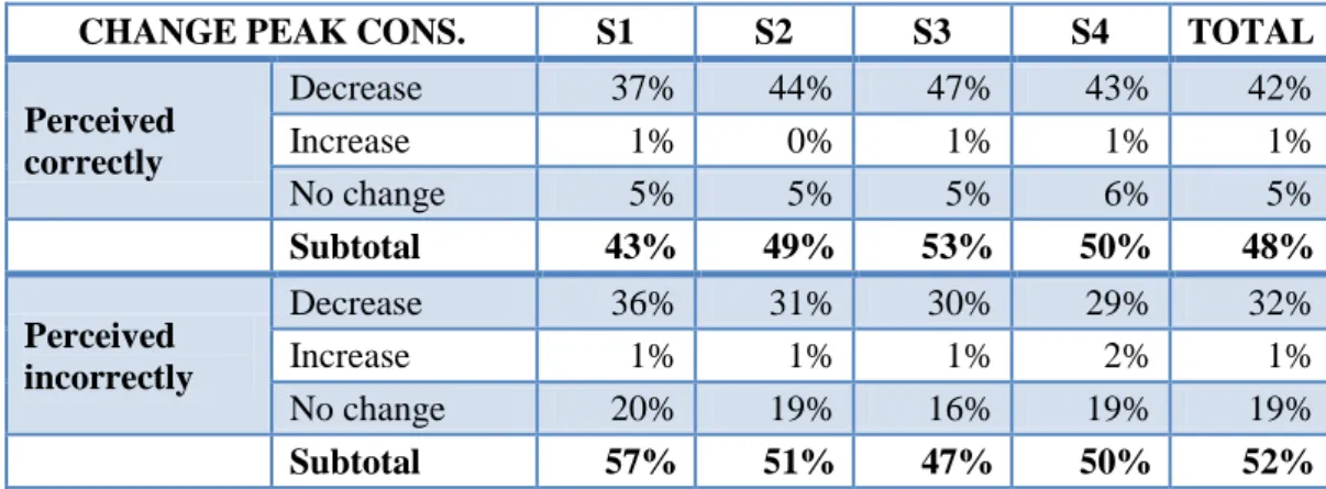
Perceived correctly Decrease 37% 44% 47% 43% 42% Increase 1% 0% 1% 1% 1% No change 5% 5% 5% 6% 5% Subtotal 43% 49% 53% 50% 48% Perceived incorrectly Decrease 36% 31% 30% 29% 32% Increase 1% 1% 1% 2% 1% No change 20% 19% 16% 19% 19% Subtotal 57% 51% 47% 50% 52%

Table 7- Perception of change in peak consumption during the trial

Table 7 refers to the perceptions of change in peak consumption. The first half of the table shows the percentage of participants with correct perceptions (correctly aligned with the real values) of a decrease, an increase or no change. The second half reflects the portion of participants that perceived incorrectly a decrease, an increase or no change when they obtained other outcome in reality. A Pearson’s chi-square test was performed to discover if the null hypothesis that there was homogeneity between the results of the different stimuli could be rejected, and therefore the analysis could be executed. For the perception of change in peak consumption with the trial the null hypothesis was accepted, meaning that the outcomes were equally likely to occur. Conversely, for the perceptions of change in overall usage and bills the null hypothesis was rejected, so the results are interpreted below.

CHANGE OVERALL CONS. S1 S2 S3 S4 TOTAL

Perceived correctly Decrease 21% 25% 29% 25% 25% Increase 2% 1% 3% 1% 2% No change 12% 9% 9% 14% 11% Subtotal 35% 35% 41% 40% 38% Perceived incorrectly Decrease 36% 40% 38% 36% 37% Increase 2% 1% 1% 2% 1% No change 27% 24% 20% 22% 24% Subtotal 65% 65% 59% 60% 62%

(23)

23

From Table 8, above, we can realize that from the totality of 2570 test group participants, 62% did not perceive correctly the change in their overall consumption. Stimuli 1 and 2 had less participants perceiving correctly (35% for both) and more perceiving incorrectly the change in consumption (65%). Stimuli 3 and 4 achieved, however, better results. Most participants claimed to have had a decrease in overall consumption during the trial, 25 % correctly and 37% incorrectly. Also, a fairly large percentage of consumers believed incorrectly that they had achieved no change in overall usage (24%).

CHANGE BILL S1 S2 S3 S4 TOTAL

Perceived correctly Decrease 24% 29% 32% 28% 28% Increase 4% 2% 3% 2% 3% No change 9% 7% 7% 13% 9% Subtotal 37% 38% 42% 43% 40% Perceived incorrectly Decrease 38 % 43% 34% 37% 38% Increase 4% 3% 4% 3% 3% No change 21% 16% 20% 17% 19% Subtotal 63 % 62% 58% 57% 60%

Table 9- Perception of change in bills during the trial

For the perception of change in electricity bills very similar results to the overall consumption were achieved. Table 9 reveals more participants perceiving incorrectly the change in their costs than correctly (60% incorrectly), stimuli 1 and 2 achieving the worst results and stimuli 3 and 4 the best.

In both cases the stimuli with just the EUS and bill (stimuli 1 and 2) achieved poorer results. It seems that having an extra component besides the EUS and the bill (a monitor for Stimulus 3 and a monetary incentive to consume less for Stimulus 4) achieves better results, with more participants receiving these stimuli perceiving correctly the variations in overall consumption and bills.

(24)

24

Comparing Table 6 with Tables 8 and 9 we can notice that few consumers perceive correctly an increase of usage that happened in reality. Most participants believed they had a decrease in usage or costs when a large portion had in fact increased those. Some reasons for this phenomenon could be a lack of attention paid to the bills and EUS or because by being part of the experience they felt they could only have had positive results, decreasing their consumption.

5.2. Comparison of perception of change in consumption and bills

In the survey, after each of these questions about perception it was asked by what amount the participant believed the consumption or bill changed, with the possible answers: 1- Less than 5%; 2- Between 5% and 10%; 3- Between 10% and 20%; 4-Between 20% and 30%; 5- More than 30%; 6- Don’t know.

As previously stated, one of CER’s conclusions was that participants assumed that their change in consumption and bill was equal in percentage, forgetting the effect of the different prices per kWh of ToU tariffs. In fact, after an analysis I could confirm this result: 90% of the participants who selected the same percentage of decrease or increase for their consumption and bill did it incorrectly. This mistake was homogeneous across all stimuli with none standing out with more correct or incorrect perceptions.

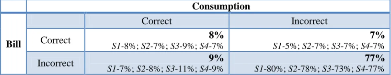
To generally understand if the participants made more mistakes estimating the percentage of change in their consumption or in their bills we may observe Table 10.

Consumption Bill Correct Incorrect Correct 8% S1-8%; S2-7%; S3-9%; S4-7% 7% S1-5%; S2-7%; S3-7%; S4-7% Incorrect 9% S1-7%; S2-8%; S3-11%; S4-9% 77% S1-80%; S2-78%; S3-73%; S4-77% Table 10- Participants' perception of change in percentage of their bills and consumption

(25)

25

Most participants estimated this change incorrectly for both bills and usage (77% of 115012). Slightly more consumers perceived incorrectly the change in bills but correctly in consumption (9%) than the reverse. Stimulus 3, compared to other stimuli, stands out with a smaller proportion of participants perceiving both incorrectly (73%) and higher of both correctly (9%).

This lack of perception, demonstrated in Tables 8, 9 and 10, can be related to the lack of knowledge of tariffs showed in Graphs 1 and 2, and to a general disinterest by participants in understanding their bills and consumptions. This constitutes a problem as it could move consumers away from trying to attain better results and save more energy.

6. Conclusion

The successful Smart metering trials in the Republic of Ireland, which combined ToU tariffs with DSM stimuli, produced a wide list of conclusions about the consumer behavior of the participants. Yet, there was still room for additional studies in order to clarify some points. The regression analyses performed in this report revealed that different results can be obtained by conducting a multiple regression analysis instead of studying each variable alone. This demonstrates that the possibilities of analyses should be carefully exhausted before taking final conclusions.

In terms of results, this report disclosed that one of the weakest points of the trial was the lack of understanding or interest by consumers in comprehending the tariffs and questions related to consumption. This was also reflected in a very low level of the participants’ perception of their changes in usage and bills attained with the trial. Correct consumer perceptions of their results are clearly a key point for the achievement of better results and to explore the full potential of the project without obstacles caused

12_{Not all the 2570 test participants are included in this analysis as it excludes the ones that answered that}

there was no change in their bills or overall consumption and the ones that selected “Don’t know” to the question about the percentage of change.

(26)

26

by lack of knowledge. Hence a better education of the consumer, concerning these subjects, should be explored in the future.

This report has the final objective of complementing CER’s Consumer Behavior report and intends to be useful as a term of comparison for consumer behavior studies of smart metering projects performed in other countries.

7. References

1. Argyrous, George. 2005. Statistics for Research: With a Guide to SPSS. UK: Sage Publications.

2. CER. 2012. “CER-Overview” http://www.cer.ie/en/about-us-overview.aspx

3. Comission for Energy Regulation. 2011. “Electricity Smart Metering Customer Behaviour Trials (CBT) Findings Report”

4. Comission for Energy Regulation. 2011. “Appendices to the Electricity Smart Metering Customer Behaviour Trials (CBT) Findings Report”

5. Irish Social Science Data Archive. 2011. “CER Smart Metering Project”

http://www.ucd.ie/issda/data/commissionforenergyregulation/

6. Motulsky, Harvey. 2002. “Multicollinearity in multiple regression”

http://www.graphpad.com/articles/Multicollinearity.htm

7. PNAS. 2010. “Public perceptions of energy consumption savings”

http://www.pnas.org/content/early/2010/08/06/1001509107.full.pdf+html

8. UCLA: Academic Technology Services, Statistical Consulting Group. 2007. “SPSS Anotated Output Regression Analysis”