arXiv:1702.02835v1 [astro-ph.IM] 9 Feb 2017
Impact of atmospheric effects on the energy
reconstruction of air showers observed by the
surface detectors of the Pierre Auger Observatory
A. Aab63, P. Abreu70, M. Aglietta48,47, I. Al Samarai29, I.F.M. Albuquerque16,
I. Allekotte1, A. Almela8,11, J. Alvarez Castillo62, J. Alvarez-Muñiz79, G.A. Anastasi38,
L. Anchordoqui83, B. Andrada8, S. Andringa70, C. Aramo45, F. Arqueros77,
N. Arsene73, H. Asorey1,24, P. Assis70, J. Aublin29, G. Avila9,10, A.M. Badescu74,
A. Balaceanu71, R.J. Barreira Luz70, C. Baus32, J.J. Beatty89, K.H. Becker31,
J.A. Bellido12, C. Berat30, M.E. Bertaina56,47, X. Bertou1, P.L. Biermannb,
P. Billoir29, J. Biteau28, S.G. Blaess12, A. Blanco70, J. Blazek25, C. Bleve50,43,
M. Boháčová25, D. Boncioli40,d, C. Bonifazi22, N. Borodai67, A.M. Botti8,33,
J. Brack82, I. Brancus71, T. Bretz35, A. Bridgeman33, F.L. Briechle35, P. Buchholz37,
A. Bueno78, S. Buitink63, M. Buscemi52,42, K.S. Caballero-Mora60, L. Caccianiga53,
A. Cancio11,8, F. Canfora63, L. Caramete72, R. Caruso52,42, A. Castellina48,47,
G. Cataldi43, L. Cazon70, A.G. Chavez61, J.A. Chinellato17, J. Chudoba25,
R.W. Clay12, R. Colalillo54,45, A. Coleman90, L. Collica47, M.R. Coluccia50,43,
R. Conceição70, F. Contreras9,10, M.J. Cooper12, S. Coutu90, C.E. Covault80,
A. Criss90, J. Cronin91, S. D’Amico49,43, B. Daniel17, S. Dasso5,3, K. Daumiller33,
B.R. Dawson12, R.M. de Almeida23, S.J. de Jong63,65, G. De Mauro63,
J.R.T. de Mello Neto22, I. De Mitri50,43, J. de Oliveira23, V. de Souza15,
J. Debatin33, O. Deligny28, C. Di Giulio55,46, A. Di Matteo51,41, M.L. Díaz
Castro17, F. Diogo70, C. Dobrigkeit17, J.C. D’Olivo62, R.C. dos Anjos21,
M.T. Dova4, A. Dundovic36, J. Ebr25, R. Engel33, M. Erdmann35, M. Erfani37,
C.O. Escobar84,17, J. Espadanal70, A. Etchegoyen8,11, H. Falcke63,66,65, G. Farrar87,
A.C. Fauth17, N. Fazzini84, B. Fick86, J.M. Figueira8, A. Filipčič75,76, O. Fratu74,
M.M. Freire6, T. Fujii91, A. Fuster8,11, R. Gaior29, B. García7, D.
Garcia-Pinto77, F. Gatée, H. Gemmeke34, A. Gherghel-Lascu71, P.L. Ghia28, U. Giaccari22,
M. Giammarchi44, M. Giller68, D. Głas69, C. Glaser35, H. Glass84, G. Golup1,
M. Gómez Berisso1, P.F. Gómez Vitale9,10, N. González8,33, A. Gorgi48,47,
P. Gorham92, P. Gouffon16, A.F. Grillo40, T.D. Grubb12, F. Guarino54,45,
G.P. Guedes18, M.R. Hampel8, P. Hansen4, D. Harari1, T.A. Harrison12,
J.L. Harton82, Q. Hasankiadeh64, A. Haungs33, T. Hebbeker35, D. Heck33,
P. Heimann37, A.E. Herve32, G.C. Hill12, C. Hojvat84, E. Holt33,8, P. Homola67,
J.R. Hörandel63,65, P. Horvath26, M. Hrabovský26, T. Huege33, J. Hulsman8,33,
A. Kääpä31, O. Kambeitz32, K.H. Kampert31, P. Kasper84, I. Katkov32,
B. Keilhauer33, E. Kemp17, J. Kemp35, R.M. Kieckhafer86, H.O. Klages33,
M. Kleifges34, J. Kleinfeller9, R. Krause35, N. Krohm31, D. Kuempel35,
G. Kukec Mezek76, N. Kunka34, A. Kuotb Awad33, D. LaHurd80, M. Lauscher35,
P. Lebrun84, R. Legumina68, M.A. Leigui de Oliveira20, A. Letessier-Selvon29,
I. Lhenry-Yvon28, K. Link32, L. Lopes70, R. López57, A. López Casado79,
Q. Luce28, A. Lucero8,11, M. Malacari91, M. Mallamaci53,44, D. Mandat25,
P. Mantsch84, A.G. Mariazzi4, I.C. Mariş78, G. Marsella50,43, D. Martello50,43,
H. Martinez58, O. Martínez Bravo57, J.J. Masías Meza3, H.J. Mathes33,
S. Mathys31, J. Matthews85, J.A.J. Matthews94, G. Matthiae55,46, E. Mayotte31,
P.O. Mazur84, C. Medina81, G. Medina-Tanco62, D. Melo8, A. Menshikov34,
S. Messina64, M.I. Micheletti6, L. Middendorf35, I.A. Minaya77, L. Miramonti53,44,
B. Mitrica71, D. Mockler32, S. Mollerach1, F. Montanet30, C. Morello48,47,
M. Mostafá90, A.L. Müller8,33, G. Müller35, M.A. Muller17,19, S. Müller33,8,
R. Mussa47, I. Naranjo1, L. Nellen62, J. Neuser31, P.H. Nguyen12, M.
Niculescu-Oglinzanu71, M. Niechciol37, L. Niemietz31, T. Niggemann35, D. Nitz86,
D. Nosek27, V. Novotny27, H. Nožka26, L.A. Núñez24, L. Ochilo37, F. Oikonomou90,
A. Olinto91, D. Pakk Selmi-Dei17, M. Palatka25, J. Pallotta2, P. Papenbreer31,
G. Parente79, A. Parra57, T. Paul88,83, M. Pech25, F. Pedreira79, J. P¸ekala67,
R. Pelayo59, J. Peña-Rodriguez24, L. A. S. Pereira17, M. Perlín8, L. Perrone50,43,
C. Peters35, S. Petrera51,38,41, J. Phuntsok90, R. Piegaia3, T. Pierog33, P. Pieroni3,
M. Pimenta70, V. Pirronello52,42, M. Platino8, M. Plum35, C. Porowski67,
R.R. Prado15, P. Privitera91, M. Prouza25, E.J. Quel2, S. Querchfeld31,
S. Quinn80, R. Ramos-Pollan24, J. Rautenberg31, D. Ravignani8, B. Revenue,
J. Ridky25, M. Risse37, P. Ristori2, V. Rizi51,41, W. Rodrigues de Carvalho16,
G. Rodriguez Fernandez55,46, J. Rodriguez Rojo9, D. Rogozin33, M.J. Roncoroni8,
M. Roth33, E. Roulet1, A.C. Rovero5, P. Ruehl37, S.J. Saffi12, A. Saftoiu71,
H. Salazar57, A. Saleh76, F. Salesa Greus90, G. Salina46, J.D. Sanabria
Gomez24, F. Sánchez8, P. Sanchez-Lucas78, E.M. Santos16, E. Santos8, F. Sarazin81,
B. Sarkar31, R. Sarmento70, C.A. Sarmiento8, R. Sato9, M. Schauer31, V. Scherini43,
H. Schieler33, M. Schimp31, D. Schmidt33,8, O. Scholten64,c, P. Schovánek25,
F.G. Schröder33, A. Schulz33, J. Schulz63, J. Schumacher35, S.J. Sciutto4,
A. Segreto39,42, M. Settimo29, A. Shadkam85, R.C. Shellard13, G. Sigl36,
G. Silli8,33, O. Sima73, A. Śmiałkowski68, R. Šmída33, G.R. Snow93, P. Sommers90,
S. Sonntag37, J. Sorokin12, R. Squartini9, D. Stanca71, S. Stanič76, J. Stasielak67,
P. Stassi30, F. Strafella50,43, F. Suarez8,11, M. Suarez Durán24, T. Sudholz12,
T. Suomijärvi28, A.D. Supanitsky5, J. Swain88, Z. Szadkowski69, A. Taboada32,
O.A. Taborda1, A. Tapia8, V.M. Theodoro17, C. Timmermans65,63, C.J. Todero
Peixoto14, L. Tomankova33, B. Tomé70, G. Torralba Elipe79, D. Torres Machado22,
M. Torri53, P. Travnicek25, M. Trini76, R. Ulrich33, M. Unger87,33, M. Urban35,
J.F. Valdés Galicia62, I. Valiño79, L. Valore54,45, G. van Aar63, P. van Bodegom12,
A.M. van den Berg64, A. van Vliet63, E. Varela57, B. Vargas Cárdenas62,
G. Varner92, J.R. Vázquez77, R.A. Vázquez79, D. Veberič33, I.D. Vergara
Quispe4, V. Verzi46, J. Vicha25, L. Villaseñor61, S. Vorobiov76, H. Wahlberg4,
H. Wilczyński67, T. Winchen31, D. Wittkowski31, B. Wundheiler8, L. Yang76,
D. Yelos11,8, A. Yushkov8, E. Zas79, D. Zavrtanik76,75, M. Zavrtanik75,76,
A. Zepeda58, B. Zimmermann34, M. Ziolkowski37, Z. Zong28, F. Zuccarello52,42 1Centro Atómico Bariloche and Instituto Balseiro (CNEA-UNCuyo-CONICET),
Argentina
2 Centro de Investigaciones en Láseres y Aplicaciones, CITEDEF and
CON-ICET, Argentina
3 Departamento de Física and Departamento de Ciencias de la Atmósfera y
los Océanos, FCEyN, Universidad de Buenos Aires, Argentina
4 IFLP, Universidad Nacional de La Plata and CONICET, Argentina 5Instituto de Astronomía y Física del Espacio (IAFE, CONICET-UBA),
Ar-gentina
6 Instituto de Física de Rosario (IFIR) – CONICET/U.N.R. and Facultad de
Ciencias Bioquímicas y Farmacéuticas U.N.R., Argentina
7Instituto de Tecnologías en Detección y Astropartículas (CNEA, CONICET,
UNSAM) and Universidad Tecnológica Nacional – Facultad Regional Men-doza (CONICET/CNEA), Argentina
8Instituto de Tecnologías en Detección y Astropartículas (CNEA, CONICET,
UNSAM), Centro Atómico Constituyentes, Comisión Nacional de Energía Atómica, Argentina
9 Observatorio Pierre Auger, Argentina
10 Observatorio Pierre Auger and Comisión Nacional de Energía Atómica,
Ar-gentina
11 Universidad Tecnológica Nacional – Facultad Regional Buenos Aires,
Ar-gentina
12 University of Adelaide, Australia
13 Centro Brasileiro de Pesquisas Fisicas (CBPF), Brazil
14 Universidade de São Paulo, Escola de Engenharia de Lorena, Brazil 15Universidade de São Paulo, Inst. de Física de São Carlos, São Carlos, Brazil 16 Universidade de São Paulo, Inst. de Física, São Paulo, Brazil
17 Universidade Estadual de Campinas (UNICAMP), Brazil 18 Universidade Estadual de Feira de Santana (UEFS), Brazil 19 Universidade Federal de Pelotas, Brazil
20 Universidade Federal do ABC (UFABC), Brazil
21 Universidade Federal do Paraná, Setor Palotina, Brazil
22 Universidade Federal do Rio de Janeiro (UFRJ), Instituto de Física, Brazil 23 Universidade Federal Fluminense, Brazil
24 Universidad Industrial de Santander, Colombia
25 Institute of Physics (FZU) of the Academy of Sciences of the Czech
Repub-lic, Czech Republic
26 Palacky University, RCPTM, Czech Republic
27 University Prague, Institute of Particle and Nuclear Physics, Czech
Repub-lic
28Institut de Physique Nucléaire d’Orsay (IPNO), Université Paris-Sud, Univ.
29 Laboratoire de Physique Nucléaire et de Hautes Energies (LPNHE),
Uni-versités Paris 6 et Paris 7, CNRS-IN2P3, France
30Laboratoire de Physique Subatomique et de Cosmologie (LPSC), Université
Grenoble-Alpes, CNRS/IN2P3, France
31 Bergische Universität Wuppertal, Department of Physics, Germany
32 Karlsruhe Institute of Technology, Institut für Experimentelle Kernphysik
(IEKP), Germany
33Karlsruhe Institute of Technology, Institut für Kernphysik (IKP), Germany 34 Karlsruhe Institute of Technology, Institut für Prozessdatenverarbeitung
und Elektronik (IPE), Germany
35 RWTH Aachen University, III. Physikalisches Institut A, Germany 36 Universität Hamburg, II. Institut für Theoretische Physik, Germany 37 Universität Siegen, Fachbereich 7 Physik – Experimentelle Teilchenphysik,
Germany
38 Gran Sasso Science Institute (INFN), L’Aquila, Italy
39 INAF – Istituto di Astrofisica Spaziale e Fisica Cosmica di Palermo, Italy 40 INFN Laboratori Nazionali del Gran Sasso, Italy
41 INFN, Gruppo Collegato dell’Aquila, Italy 42 INFN, Sezione di Catania, Italy
43 INFN, Sezione di Lecce, Italy 44 INFN, Sezione di Milano, Italy 45 INFN, Sezione di Napoli, Italy
46 INFN, Sezione di Roma “Tor Vergata“, Italy 47 INFN, Sezione di Torino, Italy
48 Osservatorio Astrofisico di Torino (INAF), Torino, Italy 49 Università del Salento, Dipartimento di Ingegneria, Italy
50Università del Salento, Dipartimento di Matematica e Fisica “E. De Giorgi”,
Italy
51 Università dell’Aquila, Dipartimento di Scienze Fisiche e Chimiche, Italy 52 Università di Catania, Dipartimento di Fisica e Astronomia, Italy 53 Università di Milano, Dipartimento di Fisica, Italy
54 Università di Napoli “Federico II“, Dipartimento di Fisica “Ettore Pancini“,
Italy
55 Università di Roma “Tor Vergata”, Dipartimento di Fisica, Italy 56 Università Torino, Dipartimento di Fisica, Italy
57 Benemérita Universidad Autónoma de Puebla (BUAP), México
58 Centro de Investigación y de Estudios Avanzados del IPN (CINVESTAV),
México
59Unidad Profesional Interdisciplinaria en Ingeniería y Tecnologías Avanzadas
del Instituto Politécnico Nacional (UPIITA-IPN), México
60 Universidad Autónoma de Chiapas, México
61 Universidad Michoacana de San Nicolás de Hidalgo, México 62 Universidad Nacional Autónoma de México, México
63 Institute for Mathematics, Astrophysics and Particle Physics (IMAPP),
64KVI – Center for Advanced Radiation Technology, University of Groningen,
Netherlands
65 Nationaal Instituut voor Kernfysica en Hoge Energie Fysica (NIKHEF),
Netherlands
66 Stichting Astronomisch Onderzoek in Nederland (ASTRON), Dwingeloo,
Netherlands
67 Institute of Nuclear Physics PAN, Poland
68 University of Łódź, Faculty of Astrophysics, Poland
69 University of Łódź, Faculty of High-Energy Astrophysics, Poland
70 Laboratório de Instrumentação e Física Experimental de Partículas – LIP
and Instituto Superior Técnico – IST, Universidade de Lisboa – UL, Portu-gal
71 “Horia Hulubei” National Institute for Physics and Nuclear Engineering,
Romania
72 Institute of Space Science, Romania
73 University of Bucharest, Physics Department, Romania 74 University Politehnica of Bucharest, Romania
75 Experimental Particle Physics Department, J. Stefan Institute, Slovenia 76 Laboratory for Astroparticle Physics, University of Nova Gorica, Slovenia 77 Universidad Complutense de Madrid, Spain
78 Universidad de Granada and C.A.F.P.E., Spain 79 Universidad de Santiago de Compostela, Spain 80 Case Western Reserve University, USA
81 Colorado School of Mines, USA 82 Colorado State University, USA
83 Department of Physics and Astronomy, Lehman College, City University of
New York, USA
84 Fermi National Accelerator Laboratory, USA 85 Louisiana State University, USA
86 Michigan Technological University, USA 87 New York University, USA
88 Northeastern University, USA 89 Ohio State University, USA
90 Pennsylvania State University, USA 91 University of Chicago, USA
92 University of Hawaii, USA 93 University of Nebraska, USA 94 University of New Mexico, USA
a School of Physics and Astronomy, University of Leeds, Leeds, United
King-dom
b Max-Planck-Institut für Radioastronomie, Bonn, Germany c also at Vrije Universiteit Brussels, Brussels, Belgium
d now at Deutsches Elektronen-Synchrotron (DESY), Zeuthen, Germany eSUBATECH, École des Mines de Nantes, CNRS-IN2P3, Université de Nantes
Abstract
Atmospheric conditions, such as the pressure (P ), temperature (T ) or air density (ρ ∝ P/T ), affect the development of extended air show-ers initiated by energetic cosmic rays. We study the impact of the atmospheric variations on the reconstruction of air showers with data from the arrays of surface detectors of the Pierre Auger Observatory, considering separately the one with detector spacings of 1500 m and the one with 750 m spacing. We observe modulations in the event rates that are due to the influence of the air density and pressure vari-ations on the measured signals, from which the energy estimators are obtained. We show how the energy assignment can be corrected to account for such atmospheric effects.
1
Introduction
Variation of the atmospheric conditions affect the signals from the extended air shower (EAS) which can be detected at ground level with arrays of surface detectors, such as the ones of the Pierre Auger Observatory. If these effects are not understood and properly accounted for, they can induce systematic effects in the energy reconstruction of the cosmic rays (CRs). Consequently, the determination of the CR spectrum and also the search for anisotropies are affected, especially at large angular scales where the daily weather mod-ulations can induce dipolar-like anisotropies in the distribution of arrival directions (although considering time periods of several years, partial can-cellations of these modulations are expected). In an earlier investigation [1], we studied the main effects due to changes in the atmospheric condi-tions using the data from the surface detector (SD) of the Pierre Auger Observatory up to the end of August 2008. This included a total of about 106 events of all energies, with a median energy of about 0.6 EeV (where
EeV ≡ 1018 eV). Results were interpreted based on theoretical models of
shower development, validated with simulations of EAS in different atmo-spheric profiles. Those effects were already taken into account in the analyses of large scale anisotropies performed up to now [2].
In this work we improve and update the previous investigation by in-cluding events detected with a four times larger exposure. This enables us to restrict the dataset to events with energies above 1 EeV, which are less affected by trigger effects, allowing to quantify the atmospheric effects at the energies which are used in most of the physics analyses. We also in-clude data from the smaller but denser part of the array of detectors, with 750 m spacing, that was built after the completion of the 1500 m array, for which we consider events with energies above 0.1 EeV. The previous analysis
is also improved by including a delay of about two hours in the response of the atmospheric temperature at the relevant heights (of about 500 m to 1 km above ground) with respect to the changes in the temperature mea-sured at ground level. This inertia of the atmospheric response turns out to be observable with our study of the weather induced modulations of the EAS signals, and is indeed also directly observed in the atmosphere (see the Appendix). Finally, we obtain fits to the zenith angle dependence of the coefficients parameterising the weather induced modulations which are con-venient to implement a CR energy reconstruction corrected for the effects of variations in the atmospheric conditions.
2
The surface detector arrays and the data sets
The Pierre Auger Observatory is located close to the city of Malargüe in Argentina, at about 1400 m a.s.l.. An essential feature of the Observatory is its hybrid design: cosmic rays above ≃ 1017 eV are detected through the
observation of the associated air showers with arrays of surface detectors and with fluorescence telescopes overlooking the latter. A detailed description of all components is given in [3]. Since in the following we will use data from the surface detectors, we briefly recall here their main characteristics. The 1500 m array consists of 1600 water-Cherenkov detectors (WCDs) deployed on a triangular grid, covering a surface of 3000 km2. After the completion of
the 1500 m array in 2008, a denser array spaced by 750 m and covering an area of 23.5 km2, nested within the 1500 m array, was added. Comprising
61 WCDs it extends the energy range of the 1500 m array, which is fully efficient at energies above 3 EeV, down to lower energies, being fully effi-cient above 0.3 EeV. The arrays of surface detectors continuously sample the shower particles that reach the ground. The signals registered in the WCDs, due to both the electromagnetic and the muonic components of the EAS, are used to determine the core position and arrival direction of the shower and to determine an estimator of the primary energy. For the so-called ‘vertical’ events, i.e., those having zenith angles θ < 60◦
(θ < 55◦
for the 750 m ar-ray1
), a fit to the lateral distribution of the signals measured in the 1500 m array (750 m array) is performed to obtain the signal at a reference distance of 1000 m (450 m) from the core. These signals are then converted to the energy estimators S38 (S35), corresponding to the signals that would have
been expected had the shower arrived at a reference zenith angle of 38◦(35◦).
1
We will in the following often write inside parentheses the quantities associated to the 750 m array.
The conversion is performed through the method of the constant intensity cut, or CIC in short. This allows one to account for the effects of atmo-spheric attenuation exploiting the fact that the CR flux is almost isotropic, so that the rate per bin of sin2θ above a given true energy should be
essen-tially constant if the detector is fully efficient. In this way one determines a function fCIC(θ) such that S38 = S/fCIC(θ) (or S35 = S/fCIC′ (θ)). Finally,
a high-quality subset of hybrid events (i.e., detected simultaneously by the fluorescence and surface detectors) is used to calibrate the SD energy estima-tors with the energies E measured almost calorimetrically by the fluorescence telescopes. The correlations between the two SD energy estimators and E are well described by a simple power-law function: E = ASB
38 (E = A ′
SB′
35),
in terms of the calibration constants A and B (or A′ and B′) [4].
0 200 400 600 800 1000 1200 1400 01/2005 01/2007 01/2009 01/2011 01/2013 01/2015 # Active hexagons 0 5 10 15 20 25 30 35 40 45 01/2009 01/2011 01/2013 01/2015 # Active hexagons
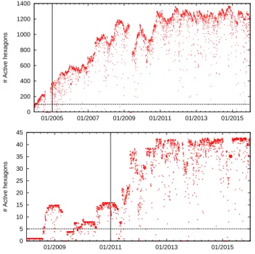
Figure 1: Evolution of the number of active hexagons of stations as a function of time for the 1500 m (top) and the 750 m (bottom) arrays. The horizontal dashed lines indicate the value corresponding to about 10% of the nominal number of hexagons: data periods for which the number of active hexagons is lower are excluded from the analysis. The vertical lines indicate the starting dates for the present analyses.
contained in the SD array are selected [5]. This fiducial criterium requires that the detector with the highest signal be enclosed in a hexagon of six active stations. The choice of a fiducial trigger based on active hexagons allows exploiting the regularity of the array to compute the effective area simply as the sum of the areas associated to all active hexagons. Each hexagon contributes a surface of √3d2/2, with d the spacing between the
detectors in the equilateral triangular grid. The evolution of the number of active hexagons over time, until the end of 2015, is shown in Figure 1 for the 1500 m array (top panel) and the 750 m array (bottom panel). The 1500 m array started its operation at the beginning of 2004; its size kept growing until its completion in 2008. The 750 m array in turn started to be deployed in 2008 and was completed in 2011. Note that, even after the deployment, the number of hexagons is not constant, due to temporary problems at the detectors (e.g., failures of electronics, power supply, communication system, etc., that are constantly monitored and accounted for in the evaluation of the effective area). In both panels, the vertical lines indicate the starting date for the data used in the present analysis. For the 1500 m array we discard the year 2004, since the array was still quite small and its operation was not very steady. For the 750 m array, in turn, we include only data posterior to January 1 2011, when the operation became more stable and the size became significant with respect to its nominal one. The horizontal dashed lines in both panels correspond to the minimum number of active hexagons that we consider in this work, i.e., 100 for the 1500 m array and 5 for the 750 m array. As the nominal number is 1380 and 42 for the 1500 m array and the 750 m array, respectively, the chosen values correspond to about 10% of the nominal ones.
Several weather stations are in operation at the Auger Observatory to monitor the atmospheric conditions, four at the different sites of the fluores-cence telescope buildings and one near the laser facility close to the centre of the 1500 m array [3]. For the present analysis, we use a database consisting of the temperature and pressure measured at the Central Laser Facility (CLF) weather station, available every 5 minutes for most of the time. When gaps in the data between 10 minutes up to three hours are present, the data are just interpolated from the values at the endpoints of those empty intervals. For the longer periods when this station is not operational, we adopt data from the other stations2
, if available, or otherwise discard the period for the 2
Since weather stations lie at different heights (the stations used are CLF at 1401 m (from which 92.8% of the atmospheric data is retrieved), Los Leones at 1420 m (3.8% of the data), Los Morados at 1423 m (3.0 % of the data) and Loma Amarilla at 1483 m (0.4% of the data)), the pressure measurements are corrected to the reference height of CLF.
850 860 870 880 01/2005 01/2007 01/2009 01/2011 01/2013 01/2015 Pd [hPa] 1 1.04 1.08 1.12 1.16 01/2005 01/2007 01/2009 01/2011 01/2013 01/2015 ρd [kg.m -3]
Figure 2: Daily averages of P (top) and ρ (bottom). present analysis.
As discussed in the next section, the most convenient way to study the atmospheric effects on EAS is by considering as variables the pressure, P , and the air density, ρ. The latter is approximately determined from the values of P and T through the dry air relation ρ ≃ 0.3484P/(T +273.16) kg m−3, with
P in hPa and T in◦
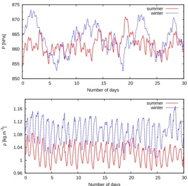
C, with the humidity having only a subdominant effect in the density near ground. In Figure 2 we show the values at the CLF location of the daily-averaged pressure (top panel) and density (bottom panel) during the time periods considered in this work, being the uncertainties in these averaged quantities negligible. In Figure 3 we plot with red lines the actual pressure and density measured every 5 min in one month during austral summer (January 2015 as an example) and with blue dashed lines in a winter month (July 2014). The seasonal modulation in the density is quite apparent, being anti-correlated with the temperature changes, so that it reaches a maximum in winter and a minimum in summer. Overall, the daily-averaged density changes by about ±6% during the year, while the changes within a
Also note that temperature differences of up to ±3 degrees can appear between stations due, e.g., to different cloud coverage, but their average effect is negligible .
850 855 860 865 870 875 0 5 10 15 20 25 30 P [hPa] Number of days summer winter 0.96 1 1.04 1.08 1.12 1.16 0 5 10 15 20 25 30 ρ [kg.m -3] Number of days summer winter
Figure 3: Measurements at the CLF weather station of P (top) and ρ (bot-tom) every 5 min over 30 days in a summer month, January 2015 (solid) and a winter month, July 2014 (dashed).
day can be ±3% (corresponding to temperature changes of ±8◦
C). Regarding the pressure, the seasonal modulation is less noticeable but its variations are more pronounced in winter times than during the summer. On a daily basis, the pressure at the Malargüe site is found to have generally a minimum in the afternoon, and a shallower local minimum in the early morning, and it is moreover significantly modulated by the movement of cold fronts and storm activity at the site, which are more frequent during winter times.
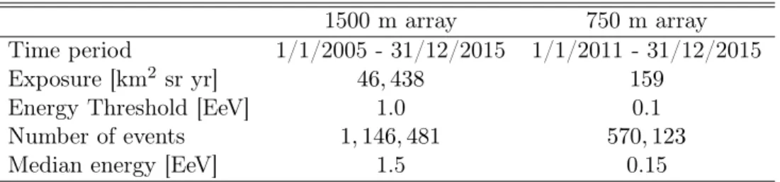
To conclude this section, we summarize in Table 1 the characteristics of the two data sets used in this work, including the time periods considered and the relative exposures. The number of events above the given energy threshold is that obtained after applying to data the selection cuts described above, based on fiducial criteria, minimum array size and data periods with measured weather data.
1500 m array 750 m array
Time period 1/1/2005 - 31/12/2015 1/1/2011 - 31/12/2015
Exposure [km2 sr yr]
46, 438 159
Energy Threshold [EeV] 1.0 0.1
Number of events 1, 146, 481 570, 123
Median energy [EeV] 1.5 0.15
Table 1: Characteristics of the data sets used in the analyses.
3
Determination of atmospheric coefficients from
the modulations of the event rate
In ref. [1] we have described in detail the effects of atmospheric variations on EAS as observed at the Pierre Auger Observatory. We remind here the aspects relevant to the analysis performed in the present work. The two atmospheric variables that mostly affect the shower development are the pressure and the air density. On the one hand, the pressure, which essentially measures the density of the vertical column of air, determines the “age” of the shower when it reaches the ground. Consequently, its variations affect the observed signals because of the attenuation of the longitudinal shower profile as the slant depth increases beyond that of the shower maximum, reducing the signal as the shower gets older. On the other hand, variations of the air density affect, via the Molière radius, the lateral spread of shower particles due to multiple Coulomb scattering of the electromagnetic component of the shower. This affects the measured signals, which become smaller as the density increases. An additional issue arises because the electromagnetic signal at the reference distance from the core is produced typically by the shower development over the last two cascade units (i.e., radiation lengths in air) before hitting the ground, corresponding to heights of 500 m to 1 km above ground level. This has two main implications. First, although the density (or temperature) variations at those heights are correlated with the ones determined at ground level, the daily amplitude of the temperature variations are smaller above ground level than at ground level, typically by a factor 1/2 to 1/3 at the relevant heights considered. Second, there is a delay of about two hours in the response of the atmosphere to the temperature variations produced by the heating or cooling of the ground. An effective way to account for these effects is to split the modulation due to the density variations into two terms: the first term is proportional to the variations of the daily averaged density, which has similar variations at ground level and
at heights of 1 km above it; the second term is proportional to the deviation of the density at a given time from the daily average, which is smaller at the relevant heights than at ground level. This daily modulation should also be retarded by about two hours in order to account for the inertia of the atmosphere to the changes in temperature determined at ground level.
For each reconstructed EAS event, the signals S at the reference distance from the shower axis of 1000 m (450 m), obtained from the fit to the lateral distribution of the signals measured in the individual WCDs, are expected to be modulated according to
S = S0[1 + αP(P − P0) + αρ(ρd− ρ0) + βρ(˜ρ − ρd)], (1)
where P0 = 862 hPa and ρ0 = 1.06 kg m−3 are reference values for P and ρ
corresponding to averages at the site of the Pierre Auger Observatory during the years considered here. S0 is the value of the signal that would have been
obtained at those reference atmospheric conditions, ρdis the daily average of
the density (within ±12 h of the event) while P and ρ are the actual pressure and density determined at ground level at the time of the event, ˜ρ being the density that was determined two hours before. The coefficients αP, αρ and
βρ parameterize the assumed linear dependence of the signal modulation.
The dependence of the signal on the atmospheric conditions leads to a modulation of the rate R of recorded events above a given signal Smin, per
unit time, area and zenith angle, which can be written as dR dθ = 2π sin θ cos θ Z ∞ Smin dS Ptr(S, θ) dΦCR dEt dEt dS , (2)
where Ptraccounts for a possible non-saturated trigger efficiency for energies
E < 3 EeV (E < 0.3 EeV), assumed to depend, for every given zenith angle, just on the signal S at the reference distance. The differential flux of cosmic rays per unit solid angle is assumed to follow a power law E−γ
t , with Et the
true energy of the CRs, and the spectral index will be taken here as γ = 3.29, as determined by the Auger Observatory [4] at energies below ∼ 5 EeV (i.e., below the ankle feature above which the spectrum hardens). This spectral index is the one relevant for this study since in the following we will consider threshold energies of 1 EeV (or 0.1 EeV for 750 m array). Using now the energy calibration relation with Et≃ AS0B in terms of the signal S0 at the
reference atmospheric conditions (as will be further discussed in Section 4) we obtain from Eq. (1), expanding to first order in the weather corrections, that
dR
d sin2θ ∝ [1+aP(P −P0)+aρ(ρd−ρ0)+bρ(˜ρ−ρd)]
Z ∞ Smin
dS Ptr(S, θ)S−Bγ+B−1.
(3) For the assumed CR energy spectrum with the shape of a power-law, the relation between the rate coefficients and the signal ones is aP,ρ = B(γ −
1)αP,ρ and similarly bρ= B(γ − 1)βρ. The coefficient B is derived from the
energy calibration [4] and is equal to B = 1.023±0.006 for the 1500 m array (B′
= 1.013 ± 0.013 for the 750 m array). One has then that aP,ρ≃ 2.3αP,ρ
and similarly bρ≃ 2.3βρ.
To determine the atmospheric coefficients we compute the rate by count-ing the events in one hour bins and normalizcount-ing to the correspondcount-ing area of the array at that time, which is calculated from the total number of hexagons of active neighboring detectors, which is known at every second.
We finally use the expression given by Eq. (3) to fit the measured rate of events. Assuming that the number of events ni observed in each hour bin
i follows a Poisson distribution of average µi, a maximum likelihood fit is
performed to estimate the coefficients aP, aρand bρ. The likelihood function
is L =Qµni
i e
−µi/n
i!. The expected number of events in bin i is given by
µi = R0× Ai× Ci,
where R0 is the average rate that would have been observed if the
atmo-spheric parameters were always the reference ones, i.e., R0 =Pni/PAiCi,
with Ai the sensitive area in the ith time bin and
Ci = 1 + aP(Pi− P0) + aρ(ρdi− ρ0) + bρ(˜ρi− ρdi),
where ˜ρi = ρi−2 means that the density used in the fitting procedure is the
one measured two hours before.
3.1 Results for the 1500 m array
For the 1500 m array a first analysis was performed in ref. [1] using data from January 1 2005 up to August 31 2008, with no energy selection other than that imposed by the trigger, corresponding to about 106 events with
median energy of about 0.6 EeV. We here extend this dataset up to the end of 2015. Given the much larger statistics available it becomes possible to determine the atmospheric coefficients using a higher threshold of 1 EeV, with a median of about 1.5 EeV, so that the rates are less affected by trigger effects at energies below full trigger efficiency. This also leads to coefficients
determined in an energy range which is closer to the energies at which the physics analyses are performed. One has to keep in mind that the coefficients may depend on the energy, due e.g., to the logarithmic energy dependence of the depth of shower maximum, the possible energy dependence of the slope of the lateral distributions of signals measured at ground or of the electro-magnetic fraction of the shower, or even due to changes in the predominant CR composition at different energies. Anyhow, this energy dependence is not expected to be large, so that even at the highest energies the correction performed using the coefficients determined close to the EeV should already account for most of the effects.
0.1 0.12 0.14 0.16 0.18 0.2 0.22 0.24 01/2005 01/2007 01/2009 01/2011 01/2013 01/2015
Rate of events [day
-1km -2] 0.156 0.159 0.162 0.165 0.168
Rate of events [day
-1km -2]
Data Expected with 2 hr delay Expected without delay
-0.003 0 0.003
0 4 8 12 16 20 24
Residuals
Hour of the day (Local Time)
Figure 4: Top panel: Rate of events per day, with E > 1 EeV, for the 1500 m array. The experimental points are shown in red while the black points represent the expectations from the fit. Bottom panel: Average hourly measured rates and expectations from the fit including the two hour delay (squares) or with the actual density (triangles), with their residuals.
We first perform a fit to the atmospheric coefficients including all zenith angles, θ < 60◦, by using Eq. (3) to fit the rate of events with E > 1 EeV in
) θ ( 2 sin 0 0.2 0.4 0.6 ] -1 [hPaP a 0.006 − 0.005 − 0.004 − 0.003 − 0.002 − 0.001 − 0 0.001 0.002 ) θ ( 2 sin 0 0.2 0.4 0.6 ] 3 m -1 [kgρ a 2.5 − 2 − 1.5 − 1 − 0.5 − 0 ) θ ( 2 sin 0 0.2 0.4 0.6 ] 3 m -1 [kgρ b 1 − 0.8 − 0.6 − 0.4 − 0.2 − 0
Figure 5: Atmospheric coefficients aP (left), aρ (middle) and bρ (right) as a
function of sin2
θ, for the 1500 m array. The line is the fit obtained using a quadratic polynomial to describe the dependence on sin2θ.
one hour bins. In this way we obtain the following (zenith angle averaged) coefficients:
aP = (−3.2 ± 0.3) × 10−3 hPa−1
aρ = (−1.72 ± 0.04) kg−1m3 (4)
bρ = (−0.53 ± 0.04) kg−1m3.
All errors are the statistical ones associated to the fit. The reduced χ2
obtained is χ2/dof = 1.013 (for 88,126 degrees of freedom), where χ2 =
P
i(ni− µi)2/µi.
The behavior of the daily averaged rate (i.e., in 24 h bins) over the time period considered is shown in Figure 4, top panel (red points and correspond-ing error bars). The black points represent the rates expected accordcorrespond-ing to the coefficients derived from the fit. The agreement between measured and expected rates is evident, as expected from the goodness of the fit. The bottom panel displays the average rates as a function of the hour of the day (the local time at Malargüe corresponds to UTC–3, having no daylight saving changes over the year). Here red points with error bars are the data, squares represent the expectation from the fitted coefficients while triangles would be the expectations if one were to use in the expression in Eq. (1) the actual air density ρ rather than the density ˜ρ measured two hours before. A significant improvement is obtained when including the delay in the fit, with the reduced χ2 changing from 4.2 without delay down to 1.9 with delay
(for 21 degrees of freedom). The residuals in both cases are shown in the lower insert. It is apparent that the improvements obtained with the delay are most noticeable at the times of the day at which the temporal variation in the temperature is maximal. To guide the eye we joined with lines the
c0 c1 c2 aP [hPa−1] (2.1 ± 0.9) × 10−3 (−2.6 ± 0.6) × 10−2 (2.6 ± 0.7) × 10−2 aρ [kg −1m3] −2.7 ± 0.1 1.5 ± 0.8 2.2 ± 1.0 bρ[kg−1m3] −1.0 ± 0.1 1.2 ± 0.8 0.0 ± 1.1
Table 2: Parameters of the fits to the zenith angle dependence of the atmo-spheric coefficients for the 1500 m array, using the quadratic polynomials in Eq. (5).
points corresponding to the expectations from the model.
To study the dependence of the atmospheric coefficients on the zenith angle we divide the data set into five bins of equal width in sin2θ, so that
the number of events per bin is similar, and fit the coefficients in each subset3
. The results are shown in Figure 5, together with a fit to the zenith angle dependence of the coefficients using quadratic polynomials
f (x) = c0+ c1x + c2x2 , where x = sin2θ. (5)
Here f might be aP, aρ or bρ. The resulting values of the coefficients are
summarized in Table 2. The main features of the results obtained can be understood by noting that the pressure coefficient is negative because an increase in atmospheric pressure corresponds to an increase in the vertical column of matter traversed by the shower, hence the same EAS will be observed at a later stage of development as the pressure increases. The sig-nals are actually the superposition of the electromagnetic and the muonic components, and while the latter changes little with increasing depth, the electromagnetic one gets exponentially suppressed beyond the shower max-imum4
. For the energies considered here the shower maximum at 1000 m from the core is close to ground level for vertical showers, which explains the small value of aP for θ ≃ 0◦. For increasing zenith angles, the shower
reaches ground when the longitudinal development is already getting sup-pressed. Hence, the energy estimator becomes smaller when the pressure increases. This effect gets more pronounced as the zenith angle increases un-til for zenith angles approaching 60◦ the electromagnetic component starts
3
Note that a binning in sin2θ is also used to fit the CIC functional dependence. In
ref. [1] we used instead bins in secθ, but this leads to significantly smaller number of events, and hence larger statistical errors, for large values of secθ.
4
Moreover, the maximum of the electromagnetic component at 1000 m from the core
is deeper by about 100 g cm−2 than the maximum at the core which is measured by the
to become subdominant and hence the pressure coefficient starts to become smaller in absolute value. Regarding the density coefficients, aρand bρ, they
are also negative since a larger air density reduces the lateral spread of the shower. For large zenith angles they become smaller due to the suppression of the electromagnetic fraction of the signal. One can also appreciate that the coefficient bρ is smaller than aρ by a factor of about one third, due to
the proportionally smaller amplitude of daily temperature variations at the relevant heights with respect to those at ground level.
3.2 Results for the 750 m array
Considering now the 750 m array and using Eq. (3), we fit the rate of events with E > 0.1 EeV and θ < 55◦, computed in one hour bins, to obtain
the coefficients averaged over zenith angles: aP = (−4.9 ± 0.4) × 10
−3
hPa−1
aρ = (−1.07 ± 0.06) kg−1m3 (6)
bρ = (−0.37 ± 0.06) kg−1m3.
The reduced χ2 of the fit is 0.998 (for 39,258 degrees of freedom).
The behavior of the daily averaged rate of events (i.e., in bins of 24 h) over the time period considered is shown in Figure 6, top panel (red points and corresponding error bars). The rates expected from the fit are shown as black points and the agreement with the measured rates is evident in this case too. The average hourly rate is shown in the bottom panel, with the fit including the 2 h delay (squares) leading to a χ2/dof = 1.76 (while the fit
without delay, shown with triangles, has χ2
/dof = 1.84).
To analyze the dependence on zenith angle we split the 750 m array data set in equal-width bins of sin2θ. However, due to the smaller number of
events and reduced zenith angle range we use in this case just three bins. The resulting atmospheric coefficients are thus fitted to linear functions
g(sin2θ) = c0+ c1sin2θ. (7)
The results are displayed in Figure 7, with the best fit parameters being listed in Table 3. By comparing the results with those of the 1500 m array, one finds similar features. The smaller values of aρfound in the 750 m array
case can be understood because logarithmic slope of the lateral distribution function is indeed smaller at distances from the core smaller than ∼ 700 m than at larger distances [3]. Hence, the density coefficient is smaller when
12 14 16 18 20 22 24 26 28 30 32 01/2011 01/2012 01/2013 01/2014 01/2015 01/2016
Rate of events [day
-1km -2] 20.2 20.4 20.6 20.8 21 21.2 21.4 21.6
Rate of events [day
-1km -2]
Data Expected with 2 hr delay Expected without delay
-0.4 0 0.4
0 4 8 12 16 20 24
Residuals
Hour of the day (Local Time)
Figure 6: Top panel: Rate of events per day, with E > 0.1 EeV, for the 750 m array. The black points represent the expected rates according to the fit. Bottom panel: Average hourly measured rates and expectations from the fit (squares) and the residuals. Triangles would be the results not including the 2 h delay in the densities.
the signal is evaluated at 450 m than when it is evaluated at 1000 m. Also from the comparison of the average coefficients of the 1500 m array in Eq. (5) and those of the 750 m array in Eq. (7) we see that the relative importance of the pressure effects is larger for the 750 m array. The subdominant effect of the density variations, together with the still relatively large error bars, also explains the reduced improvement in the fit achieved with the 2 h delay.
) θ ( 2 sin 0 0.1 0.2 0.3 0.4 0.5 0.6 ] -1 [hPaP a 0.008 − 0.007 − 0.006 − 0.005 − 0.004 − 0.003 − 0.002 − 0.001 − 0 ) θ ( 2 sin 0 0.1 0.2 0.3 0.4 0.5 0.6 ] 3 m -1 [kgρ a 1.6 − 1.4 − 1.2 − 1 − 0.8 − 0.6 − 0.4 − 0.2 − 0 ) θ ( 2 sin 0 0.1 0.2 0.3 0.4 0.5 0.6 ] 3 m -1 [kgρ b 0.5 − 0.4 − 0.3 − 0.2 − 0.1 − 0
Figure 7: Atmospheric coefficients aP (left), aρ (middle) and bρ (right) as a
function of sin2
θ, for the 750 m array. The line is the fit obtained assuming a linear dependence on sin2θ.
c0 c1 aP [hPa −1 ] (−2.5 ± 0.8) × 10−3 (−0.8 ± 0.2) × 10−2 aρ [kg−1m3] −1.6 ± 0.1 1.8 ± 0.3 bρ [kg −1m3] −0.4 ± 0.1 0.1 ± 0.3
Table 3: Coefficients of the fit to the zenith angle dependence of the atmo-spheric coefficients for the 750 m array, using a linear function as in Eq. (7).
4
Atmospheric effects on the energy reconstruction
In the previous section we discussed how the signal S at the reference dis-tance (at 1000 m for 1500 m array and at 450 m for 750 m array) is mod-ulated by the changes in the atmospheric variables that affect the shower development. These effects in turn imply that the rate of events above a given uncorrected signal (or energy) is modulated by the variations in the atmospheric conditions, and we exploited this to obtain the coefficients aP, aρ and bρ parameterizing the rate modulations. As discussed before,
the coefficients modulating the signals themselves, see Eq. (1), are given by αP,ρ= aP,ρ/[B(γ −1)] and βρ= bρ/[B(γ −1)], where γ ≃ 3.29 is the spectral
index of the CR flux below the ankle energy and B ≃ 1.02 is related to the energy calibration.
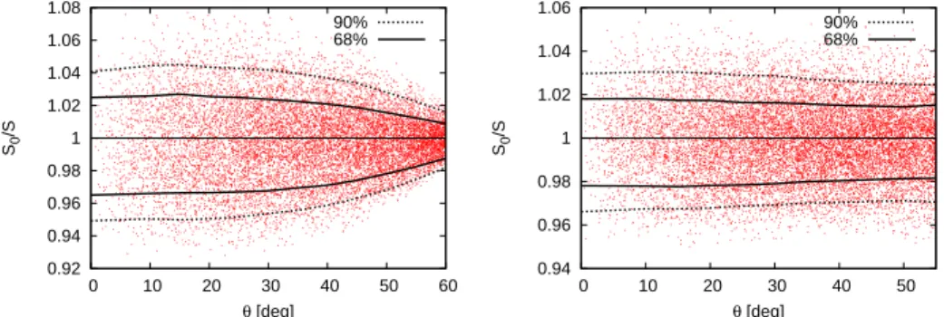
To illustrate the impact of the atmospheric effects, we show in Figure 8 the ratio between the corrected and uncorrected signals, S0/S, as a function
of the zenith angle, for both the 1500 m (left panel) and 750 m (right panel) arrays. Only events recorded in 2015 are used in the two plots, as examples, with the behavior in other years being similar. Events with E > 3 EeV are
included in the left panel, and with E > 0.3 EeV in the right panel. Given the zenith angle dependence of the atmospheric coefficients, the main effect determining the maximum amplitude of the signal correction turns out to be due to the density effect for small zenith angles, while it is instead the pressure effect for large zenith angles. Corrections to the signal, and hence to the event energy, can reach the 7% level for extreme weather variations, but are in general at the few percent level for the bulk of the events.
0.92 0.94 0.96 0.98 1 1.02 1.04 1.06 1.08 0 10 20 30 40 50 60 S0 /S θ [deg] 90% 68% 0.94 0.96 0.98 1 1.02 1.04 1.06 0 10 20 30 40 50 S0 /S θ [deg] 90% 68%
Figure 8: Ratio between the signal after (S0) and before (S) corrections, as
a function of the zenith angle, for the 1500 m array (left) and the 750 m array (right). Also shown are the contours containing 68% and 90% of the values at each zenith angle.
To arrive at a final expression for the energy reconstruction after correct-ing the signal S by atmospheric effects, the next steps would be to implement the CIC procedure in terms of S0 and then to obtain the calibration
coeffi-cients for the energy. While the implementation of such procedures is beyond the scope of the present work, we discuss them here in a general way. For definiteness we will focus below on the quantities relevant for the 1500 m array, but the discussion is completely analogous for the case of the 750 m array.
The CIC procedure assigns to each signal S from a shower arriving at a given zenith angle θ, a reference signal S38 ≡ S/fCIC(θ), which is the
signal that would have been expected from the same CR had it arrived at a reference zenith angle of 38◦ (the median zenith of the vertical events
with θ < 60◦). The function f
CIC accounts for the attenuation effects of
the atmosphere, and is usually parameterized as a cubic polynomial in the variable x ≡ cos2
θ − cos238◦: f
CIC= 1 + bx + cx2+ dx3. It is determined
using only events with energies above the minimum energy for which the array is fully efficient, so as to avoid problems due to trigger issues. It is
obtained by considering bins of equal width in sin2
θ and determining the minimum values of S in each bin above which there is a given number of events, the same for every bin. These minimum signal values are then fitted with the function g(x) = a fCIC(x). In particular, the parameter a turns out
to be approximately the minimum value of S in the central bin that includes θ = 38◦ (i.e., at x = 0). Once atmospheric effects are accounted for, one has
to consider the signals S0, at the reference atmospheric conditions P0and ρ0,
rather than the signal S, and one has to repeat the CIC procedure in terms of these corrected signals. Given the linearity of the atmospheric correction it turns out that the CIC function obtained from S0 is not significantly
modified with respect to that obtained from S if the reference atmospheric variables coincide with the overall averages. Since we here initially adopted as reference values for P0 and ρ0 the average ones, the CIC coefficients turn
out then to be essentially unchanged. If one were to adopt instead different reference conditions, the CIC fitting function would be expected to change because the atmospheric corrections do depend on zenith angle.
Regarding the energy calibration, it is performed using hybrid events measured simultaneously by the surface detectors and the fluorescence tele-scopes. Here one relates the energy E determined directly by the fluorescence telescopes, which is essentially a calorimetric measurement of the electromag-netic component of the shower, to the reference signal S38determined by the
surface detectors. From the observed hybrid events one fits the results to the relation E = ASB
38 and from it one can then assign an energy to
ev-ery EAS. Repeating this procedure in terms of the signals S0 corresponding
to the reference atmospheric conditions should in principle modify the cal-ibration coefficients A and B. The main expected effect is due to the fact that the fluorescence measurements are performed during the night, so that the average temperature of the hybrid events is about 6◦C smaller than the
average temperature of all the SD events (pressure effects should be on av-erage quite similar during nights and days). This implies that the avav-erage air density of the events used in the calibration is about 2% higher than the average air density for all the events (corresponding to a density difference of 0.02 kg m−3). Note however that when averaging the atmospheric
correc-tions to the energies, the one proportional to αρ, involving ρd− ρ0, will be
similar in the SD and FD samples, because the daily average temperatures are not much different in the two samples (just slightly lower for the hy-brid events due to the longer duration of the winter nights, which enhances the proportion of FD events collected during the winter). Hence, the rele-vant effect when comparing the average energies will be the one due to the daily modulations determined by the coefficient βρ, involving ˜ρ − ρd. Since
0.018 0.022 0.026 0.03
01/2005 01/2007 01/2009 01/2011 01/2013 01/2015
Rate of events [day
-1km -2] Corrected Energy 0.018 0.022 0.026 0.03 01/2005 01/2007 01/2009 01/2011 01/2013 01/2015
Rate of events [day
-1km -2]
Uncorrected Energy
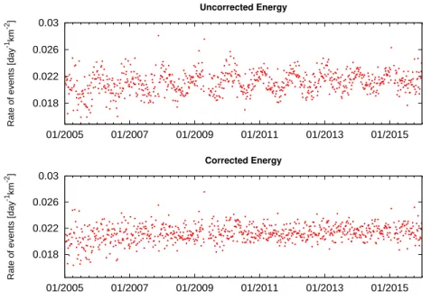
Figure 9: Daily rates before (top) and after (bottom) the correction of ener-gies for a threshold of 2 EeV for the 1500 m array.
on average βρ ≃ −0.25 kg−1m3, the signals S turn out to be about 0.5%
smaller on average for hybrid events than for all the events. These effects mostly affect the coefficient A in the calibration, which should get reduced by about ∼ 0.5% when the calibration is expressed in terms of the signals S0 at the reference atmospheric conditions. On the other hand, this is not
expected to affect the coefficient B significantly. As a result, the inclusion of atmospheric effects in the calibration is expected to lower the average of the energies assigned to the events by about 0.5% (the precise factor depending on the zenith angle). Note that this offset is anyhow much smaller than the overall systematic uncertainties in the SD energy reconstruction, which are of about 14%. One should also mention that changing the reference atmospheric variables P0 and ρ0 should affect both the CIC function and
the calibration constants, besides the zenith angle dependent atmospheric coefficients. Anyhow, the final energy assignment should be essentially in-dependent of the particular choice adopted. A detailed implementation of these procedures will be performed in a future work.
As a final check to verify that the atmospheric correction of the signal removes the systematic effects due to variations in the atmospheric condi-tions, we show in figures 9 and 10 the modulation in the daily and hourly
0.042 0.043 0.044 0.045 0.046 0 4 8 12 16 20 24
Rate of events [day
-1km -2] Uncorrected Energy 0.042 0.043 0.044 0.045 0.046 0 4 8 12 16 20 24
Rate of events [day
-1km -2]
Hour of the day (Local Time) Corrected Energy
Figure 10: Hourly rates before (top) and after (bottom) the correction of en-ergies for a threshold of 2 EeV for the 1500 m array. For guidance, horizontal lines indicate the average values.
rates, respectively, above 2 EeV (which is a threshold close to full efficiency and still leading to significant number of events), using both the uncorrected energies (top panel) and the ones corrected for atmospheric effects5
(bot-tom panel). In this last case the rates are essentially flat and the previously existing modulation has been removed.
We have also checked that the first harmonic modulation of the rates at the solar frequency have a typical amplitude of ∼ 3.5% without correc-tions. This is due to the fact that the energies are overestimated during the afternoons, when the temperature reaches a maximum, and underestimated during the early mornings, when the temperature drops. This artificial mod-ulation indeed disappears when the atmospheric corrections are included in the energy assignments.
5
For definiteness we here adopted B = 1.02 and used the CIC obtained in terms of the uncorrected signals, which should provide a very good approximation.
5
Conclusions
We have discussed in this work how to understand and correct the effects due to changes in the atmospheric variables that have an impact on the development of EAS. We have analyzed here the data from the two arrays of WCDs of the Pierre Auger Observatory, the 1500 m array and the 750 m array. The impact of the atmospheric effects depends on the way in which the reconstruction is performed, and in particular on the reference distance from the shower axis adopted to obtain the signal that is used as an energy estimator, being 1000 m for the 1500 m array and 450 m for the 750 m array. We have parameterized the dependence of this signal on the variations of air density and atmospheric pressure so as to be able to account for these effects. While the energy estimator of individual events may be affected at the few percent level by the variations of the atmospheric conditions, the average energy of all events is expected to be affected by no more than ∼ 0.5%. The results of this work will be used in the future to improve the assignment of the energy of the events detected with both arrays.
Acknowledgments
The successful installation, commissioning, and operation of the Pierre Auger Observatory would not have been possible without the strong commitment and effort from the technical and administrative staff in Malargüe. We are very grateful to the following agencies and organizations for financial sup-port:
Argentina – Comisión Nacional de Energía Atómica; Agencia Nacional de Promoción Científica y Tecnológica (ANPCyT); Consejo Nacional de In-vestigaciones Científicas y Técnicas (CONICET); Gobierno de la Provin-cia de Mendoza; Municipalidad de Malargüe; NDM Holdings and Valle Las Leñas; in gratitude for their continuing cooperation over land access; Australia – the Australian Research Council; Brazil – Conselho Nacional de Desenvolvimento Científico e Tecnológico (CNPq); Financiadora de Es-tudos e Projetos (FINEP); Fundação de Amparo à Pesquisa do Estado de Rio de Janeiro (FAPERJ); São Paulo Research Foundation (FAPESP) Grants No. 2010/07359-6 and No. 1999/05404-3; Ministério de Ciência e Tecnologia (MCT); Czech Republic – Grant No. MSMT CR LG15014, LO1305 and LM2015038 and the Czech Science Foundation Grant No. 14-17501S; France – Centre de Calcul IN2P3/CNRS; Centre National de la Recherche Scientifique (CNRS); Conseil Régional Ile-de-France;
ment Physique Nucléaire et Corpusculaire (PNC-IN2P3/CNRS); Départe-ment Sciences de l’Univers (SDU-INSU/CNRS); Institut Lagrange de Paris (ILP) Grant No. LABEX ANR-10-LABX-63 within the Investissements d’Avenir Programme Grant No. ANR-11-IDEX-0004-02; Germany – Bun-desministerium für Bildung und Forschung (BMBF); Deutsche Forschungsge-meinschaft (DFG); Finanzministerium Baden-Württemberg; Helmholtz Al-liance for Astroparticle Physics (HAP); Helmholtz-Gemeinschaft Deutscher Forschungszentren (HGF); Ministerium für Innovation, Wissenschaft und Forschung des Landes Nordrhein Westfalen; Ministerium für Wissenschaft, Forschung und Kunst des Landes Baden-Württemberg; Italy – Istituto Nazionale di Fisica Nucleare (INFN); Istituto Nazionale di Astrofisica (INAF); Ministero dell’Istruzione, dell’Universitá e della Ricerca (MIUR); Gran Sasso Center for Astroparticle Physics (CFA); CETEMPS Center of Excellence; Ministero degli Affari Esteri (MAE); Mexico – Consejo Nacional de Ciencia y Tecnología (CONACYT) No. 167733; Universidad Nacional Autónoma de México (UNAM); PAPIIT DGAPA-UNAM; The Netherlands – Ministerie van Onderwijs, Cultuur en Wetenschap; Ned-erlandse Organisatie voor Wetenschappelijk Onderzoek (NWO); Stichting voor Fundamenteel Onderzoek der Materie (FOM); Poland – National Cen-tre for Research and Development, Grants No. ERA-NET-ASPERA/01/11 and No. ERA-NET-ASPERA/02/11; National Science Centre, Grants No. 2013/08/M/ST9/00322, No. 2013/08/M/ST9/00728 and No. HARMONIA 5 – 2013/10/M/ST9/00062; Portugal – Portuguese national funds and FEDER funds within Programa Operacional Factores de Competitividade through Fundação para a Ciência e a Tecnologia (COMPETE); Romania – Roma-nian Authority for Scientific Research ANCS; CNDI-UEFISCDI partnership projects Grants No. 20/2012 and No.194/2012 and PN 16 42 01 02; Slove-nia – SloveSlove-nian Research Agency; Spain – Comunidad de Madrid; Fondo Europeo de Desarrollo Regional (FEDER) funds; Ministerio de Economía y Competitividad; Xunta de Galicia; European Community 7th Framework Program Grant No. FP7-PEOPLE-2012-IEF-328826; United Kingdom – Sci-ence and Technology Facilities Council; USA – Department of Energy, Con-tracts No. DE-AC02-07CH11359, No. DE-FR02-04ER41300, No. DE-FG02-99ER41107 and No. de-sc0011689; National Science Foundation, Grant No. 0450696; The Grainger Foundation; Vietnam – NAFOSTED; Marie Curie-IRSES/EPLANET; European Particle Physics Latin American Network; Eu-ropean Union 7th Framework Program, Grant No. PIRSES-2009-GA-246806; and UNESCO.
A
Time delay in the temperature modulation of the
atmosphere above ground level
The daily temperature modulation, both its amplitude and phase, is known to depend on the considered height above ground level, and this dependence is also different for different sites [6]. It is interesting to check how the modulations in the atmospheric conditions at different heights are related to those at ground level as a function of time at the Malargüe site. For this purpose we consider data from the Global Data Assimilation System (GDAS), a global atmospheric model which provides the main state variables as a function of the height above sea level every three hours (see [7]). A full year from December 21 2009 to December 21 2010 of temperature data at several altitudes is taken as an example. An average of the temperatures at a given height is calculated for each available hour (shown in Figure 11 for four different altitudes, with the 1400 m one corresponding to mean altitude of the Auger site). We also perform a fit to a periodic function in time of the form T (t) = hT i + A cos[π(t − td)/12 h]. The results of these fits
are summarized in Table 4. It is apparent that as the height above ground level is increased the modulation shifts to the right. The shift between the modulation at 1400 m and that at the higher altitudes is about two hours. This is an indication that for the heights relevant for the effects on EAS observed at ground (approximately two radiation lengths, corresponding to about 700 m cos θ above ground) the daily modulation of the temperature gets delayed by about two hours with respect to that measured at ground level.
Hour [Local Time]
0 2 4 6 8 10 12 14 16 18 20 22 24 C] ° T [ 2 4 6 8 10 12 14 16 18 20 1400m 2000m 2400m 2950m
Figure 11: Temperature vs. hour of the day in Malargüe, measured in Local Time, for different altitudes above sea level.
One may also note from the figure how the amplitude A of the daily temperature variations decreases with increasing height.
height [m] hT i [◦C] A [◦C] td [h] 1400 12.4 ± 0.1 5.6 ± 0.2 17.5 ± 0.1 2000 9.5 ± 0.1 2.1 ± 0.2 19.2 ± 0.3 2400 7.0 ± 0.1 1.4 ± 0.2 19.4 ± 0.4 2950 3.7 ± 0.1 0.9 ± 0.1 19.6 ± 0.6
Table 4: Parameters of the fit to temperature data from GDAS at different heights above sea level (see text).
References
[1] J. Abraham et al. (The Pierre Auger Collaboration), Atmospheric ef-fects on extensive air showers observed with the surface detector of the Pierre Auger observatory, Astroparticle Physics 32 (2009) 89 [astro-ph.IM/0906.5497v2]
[2] A. Aab et al. (The Pierre Auger Collaboration), Large scale distri-bution of ultra high energy cosmic rays detected at the Pierre Auger Observatory with zenith angles up to 80 degrees, ApJ 802 (2015) 111 [astro-ph.HE/1411.6953] ; A. Aab et al. (The Pierre Auger and Tele-scope Array Collaborations), Searches for Large-Scale Anisotropy in the Arrival Directions of Cosmic Rays above 10ˆ19 eV at the Pierre Auger Observatory and the Telescope Array, ApJ 794 (2014) 172 [astro-ph.HE/1409.3128] ; P. Abreu et al. (The Pierre Auger Collaboration), Constraints on the origin of cosmic rays above 10ˆ18 eV from large scale anisotropy searches in data of the Pierre Auger observatory, ApJL 762 (2013) L13; P. Abreu et al. (The Pierre Auger Collaboration), Large scale distribution of arrival directions of cosmic rays detected above 10ˆ18 eV at the Pierre Auger Observatory, Astrophysical Journal Supplement 203 (2012) 34 [astro-ph.HE/1210.3736v2]; P. Abreu et al. (The Pierre Auger Collaboration), Search for First Harmonic Modula-tion in the Right Ascension DistribuModula-tion of Cosmic Rays Detected at the Pierre Auger Observatory, Astropart. Phys. 34 (2011) 627 [astro-ph.HE/1103.2721]
[3] A. Aab et al. (The Pierre Auger Collaboration), The Pierre Auger Cos-mic Ray Observatory, NIM A 798 (2015) 172 [astroph.HE/1502.01323]
[4] I. Valiño for The Pierre Auger Collaboration, The flux of ultra-high energy cosmic rays after ten years of operation of the Pierre Auger Observatory, 34th ICRC The Hague The Netherlands (2015) 9
[5] J. Abraham et al. (The Pierre Auger Collaboration), Trigger and aper-ture of the surface detector array of the Pierre Auger Observatory, NIM A 613 (2010) 29 [astro-ph.IM/1111.6764]
[6] D.J. Seidel, M. Free and J. Wang, Diurnal cycle of upper-air tempera-ture estimated from radiosondes, J. of Geophys. Res. 110 (2005) D09102 [7] P. Abreu et al. (The Pierre Auger Collaboration), Description of Atmo-spheric Conditions at the Pierre Auger Observatory using the Global Data Assimilation System (GDAS), Astroparticle Physics 35 (2012) 591 [astro-ph.HE/1201.2276v2]