Cleaning of macro and micro tubes
using slug flow
A thesis submitted in part fulfilment of the requirement for the degree of Doctor in Doctoral Program in Chemical and Biological Engineering, Faculty of Engineering, by
Mónica Cristina Ferreira da Silva
Supervised by:
Doctor José Daniel Pacheco Araújo
Professor João Bernardo Lares Moreira de Campos at Centro de Estudos de Fenómenos de Transporte
Departamento de Engenharia Química Faculdade de Engenharia da Universidade do Porto
Porto, Portugal November 2018
ii Mónica Cristina Ferreira da Silva
This thesis was developed for the Doctoral Program in Chemical and Biological Engineering, at:
Departamento de Engenharia Química
Faculdade de Engenharia da Universidade do Porto Rua Dr. Roberto Frias, s/n, 4200-465, Porto, Portugal www.fe.up.pt
The work was developed in Centro de Estudos de Fenómenos de Transporte supervised by: José Daniel Pacheco Araújo
Departamento de Engenharia Química
Faculdade de Engenharia da Universidade do Porto Rua Dr. Roberto Frias, s/n, 4200-465, Porto, Portugal and
João Bernardo Lares Moreira de Campos [email protected]
This thesis was funded by FEDER funds through the Operational Programme for Competitiveness Factors COMPETE and National Funds through FCT (Fundação para a Ciência e a Tecnologia) by Ph.D. Grant
PD/BD/ 52622/2014
.iv
Acknowledgments
This work would not be possible without the help and guidance of Professors João Campos and José Daniel Araújo. I would like to thank them for their continued support and for teaching me the finer details of fluid mechanics and introducing me to the CFD techniques. In addition to the academic support, I would also like to acknowledge their availability, friendship and patience, which made this journey easier.
I would also like to thank Dr João Mário Miranda for his useful insights that helped unlock the solutions to some of the problems faced along the way.
To all members of CEFT team, in special Ana, Filipe Direito, João Carneiro, Soraia Neves for their companionship and for providing a friendly workplace.
A special thanks to Prof. José Manuel Silva for being a friend and source of inspiration.
I would also like to thank all my friends, in particular, Filipa, Joana, Luís, Miguel, Marisa, and Rita for all of their support, mostly over lunch.
To my parents and brother for helping me, since day one, in every possible way and, in doing so, allowing me to reach this far.
Finally, a special thanks to João and Mimi for always being there for me, there is not enough words to thank you.
vi
Abstract
Slug flow is a particular flow pattern that plays an important role in industrial and natural systems. This flow pattern is characterized by the presence of very large gas bubbles (Taylor bubbles) followed by liquid slugs. The surroundings of a Taylor bubble are composed by regions with different hydrodynamic characteristics: the nose includes the bubble front region; a liquid film develops between the bubble and the channel wall; and below the bubble tail normally appears a wake region. Due to its inherent hydrodynamic features, slug flow brings several advantages like the possibility to enhance mass transfer rates. The work presented in this thesis relied on Computational Fluid Dynamics (CFD) techniques to study the effect of the presence of a Taylor bubble in two phenomena: wall-liquid mass transfer and bubble-liquid mass transfer. To address this problem, both hydrodynamic and concentration fields were solved simultaneously and coupled with the Volume of Fluid (VOF) methodology to capture the gas-liquid interface. Since slug flow is a frequent gas-liquid flow pattern in macro and micro-scales systems, this study was focused on both, conventional and small size channels.
The study was planned to cover a significant range of some characteristic dimensionless numbers in both scales (different Reynolds and Capillary numbers for specific Morton numbers). For macro-scale all the cases solved were under the laminar regime.
Three sub-patterns associated to the different flow behaviors identified in micro-scales slug flow were addressed: liquid phase with no recirculation zones (Case A); presence of a closed wake following the bubble (Case B); and recirculation zones above and below the bubble (Case C). For all simulated systems, the contributions and effects of the different zones surrounding the bubble were quantified by the determination of local and average/global mass transfer coefficients. Concentration profiles were also inspected in order to analyze the solute distribution. Regarding the first phenomenon under the scope (wall-liquid mass transfer), it was shown that the flow of a Taylor bubble drastically changes the wall shear stress. Moreover, for macro-scales, the passage of a single bubble was enough to increase the mass transfer rates by 10-20% when compared to monophasic systems. On the other hand, for micro-scales, the passage of a single bubble only improved slightly the mass transfer coefficients, where the different regions as well as the different sub-patterns associated to the liquid slug have different effects on the mass transferred.
In order to study the gas-liquid mass transfer phenomenon, the flow of an isolated Taylor bubble of pure oxygen through co-current liquid phase was considered and the saturation concentration was imposed at the gas-liquid interface. Again, the impact of the different hydrodynamic regions on mass transfer was analyzed separately. For macro-scales, the higher mass transfer coefficients are associated to the film region. In this region the coefficients tend to become constant as the film gets fully developed (Ls/D<8). In the systems under consideration, the closed wake following
vii
the Taylor bubble accumulates solute with time and transports it along the domain. The mass transfer coefficients were compared with correlations based on the Higbie theory and the film theory. Between these two and for the conditions under study, the film theory seems to be the appropriate one to predict the concentration gradients near the interface.
For micro-scales, the effect of the bubble, film velocity and liquid flow sub-patterns have proven themselves essential to characterize the mass transfer phenomena. For all cases, the liquid film is the zone that shows the highest mass transfer coefficients. The solute distribution depends on the type of sub-pattern present: it is dispersed backwards (Case A), accumulated in the closed wake structure (Case B), or dispersed radially along the film region (Case C). Once again, the results were compared with the correlations available in the literature. The numerical mass transfer coefficients from Case C are in good agreement with the correlations available based on the penetration theory.
The present document clearly shows that the introduction of a Taylor bubble in a monophasic system enhances either wall-liquid mass transfer as gas-liquid mass transfer and so it may increase the velocity of chemical reactions near the wall. Furthermore, in a real system composed by a train of bubbles, the referred effects should be amplified and become highly relevant. Although being a work supported in fundamental studies, the results obtained have a large potential of impacting several daily life scenarios, such as: cleaning of medical devices, dissolution of embolisms, prediction of the effects of surfactants and the cleaning of membranes.
viii
Sumário
O slug flow é um padrão de escoamento que desempenha um papel importante em sistemas industriais e naturais. Este padrão de escoamento é caracterizado pela presença de grandes bolhas de gás (bolhas de Taylor) seguidas por um slug líquido. Em torno de uma bolha de Taylor existem diferentes regiões com diferentes características hidrodinâmicas: o nariz inclui a região frontal da bolha; um filme líquido desenvolve-se entre a bolha e a parede do canal; abaixo da base da bolha geralmente surge uma esteira. Devido às características hidrodinâmicas inerentes deste padrão de escoamento, o slug flow introduz várias vantagens, como a possibilidade de aumentar as taxas de transferência de massa. O trabalho apresentado nesta tese contou com técnicas de Dinâmica dos Fluidos Computacional (CFD) para estudar o efeito da presença da bolha de Taylor em dois fenómenos: transferência de massa líquido-parede e transferência de massa bolha-líquido. Para resolver esse problema, os campos hidrodinâmico e de concentração foram resolvidos simultaneamente e acoplados à metodologia Volume of Fluid (VOF) para rastrear a interface gás-líquido. Como o slug flow é um padrão gás-líquido frequente em sistemas de macro e micro-escalas, este estudo focou canais convencionais e canais pequenos. Em macro-escala, todos os casos resolvidos estavam sob regime laminar.
O estudo foi estruturado para cobrir uma faixa significativa de alguns números adimensionais característicos em ambas as escalas (diferentes números de Reynolds e Capilares para números específicos de Morton). Três sub-padrões associados aos diferentes comportamentos identificados em micro-escala foram também abordados: quando a fase líquida não possui zonas de recirculação (Caso A); quando surge uma esteira fechada após a bolha (Caso B); e quando surgem zonas de recirculação acima e abaixo da bolha (Caso C). Para todos os sistemas simulados, as contribuições e os efeitos das diferentes zonas em torno da bolha foram quantificados através da determinação de coeficientes de transferência de massa locais e médios/globais. Os perfis de concentração também foram inspecionados para analisar a distribuição do soluto. Em relação ao primeiro fenómeno em estudo (transferência de massa parede-líquido), a presença de uma bolha de Taylor muda drasticamente a tensão de corte da parede que por sua vez pode afetar a transferência de massa. Para macro-escala, a passagem de uma única bolha foi suficiente para aumentar as taxas de transferência de massa em 10 a 20% quando comparadas a sistemas monofásicos. Por outro lado, para micro-escala, a passagem de uma única bolha melhorou apenas ligeiramente os coeficientes de transferência de massa, onde as diferentes regiões, bem como os diferentes sub-padrões associados ao slug líquido, tem diferentes efeitos na transferência de massa.
Para estudar o fenómeno de transferência de massa gás-líquido, considerou-se uma bolha de Taylor única contendo apenas oxigénio que se dissolve através da fase líquida que se encontra em co-corrente. A concentração de saturação foi imposta na interface gás-líquido. Novamente, o impacto das diferentes regiões hidrodinâmicas na transferência de massa foi analisado
ix
separadamente. Para a macro-escala, os maiores coeficientes de transferência de massa estão associados à região do filme. Nesta região, os coeficientes tendem a tornar-se constantes à medida que o filme se desenvolve (Ls / D <8). Nos sistemas considerados, a esteira fechada, que segue a bolha de Taylor, acumula soluto com o tempo e transporta-o ao longo do domínio. Os coeficientes de transferência de massa foram comparados com os dados por correlações baseadas na teoria de Higbie e na teoria do filme. Entre estas duas, e considerando as condições especificas em estudo, a teoria do filme parece ser a apropriada para prever os gradientes de concentração próximos à interface.
Para a micro-escala, o efeito dos sub-padrões de escoamento do liquido em torno da bolha, velocidade de filme e velocidade do líquido mostraram-se essenciais para definir os fenómenos de transferência de massa. Para todos os casos, o filme é a zona que apresenta os maiores coeficientes de transferência de massa. A distribuição do soluto depende do tipo de sub-padrão presente: ele é disperso para trás (Caso A), acumulado na esteira fechada (Caso B) ou disperso radialmente ao longo da região do filme (Caso C). Os resultados obtidos foram também comparados com as correlações disponíveis na literatura. Os coeficientes numéricos de transferência de massa do Caso C estão de acordo com as correlações disponíveis baseadas na teoria da penetração.
O presente documento mostra claramente que a introdução de uma bolha de Taylor num sistema monofásico aumenta a transferência de massa líquido-parede e gás-líquido e, por isso, pode aumentar a velocidade das reações químicas perto da parede. Além disso, num sistema real composto por uma sequência de bolhas, os efeitos referidos podem ser amplificados e tornarem-se altamente relevantes. Apesar de tornarem-ser um trabalho apoiado em estudos fundamentais, os resultados obtidos têm um grande potencial para influenciar diversos cenários como: limpeza de dispositivos médicos, dissolução de embolias, prever o comportamento de surfactantes e promover a limpeza de membranas.
x Contents
List of Figures ... xiv
List of Tables ... xxii
Chapter 1 – Introduction ... 1
1.1 Relevance and motivation ... 3
1.2 Objectives ... 7
1.3 Outline ... 8
Literature Cited ... 9
Chapter 2 – State of the art ... 13
2.1 Biofilms ... 15
2.2 Slug flow ... 17
2.2.1 Slug flow in macro-scale systems ... 20
2.2.2 Slug flow in micro-scale systems ... 25
2.3 Computational Fluid Dynamics (CFD) ... 27
2.4 Mass Transfer ... 34
2.4.1 Wall-liquid mass transfer ... 34
2.4.1.1 Macro-scale systems ... 34
2.4.1.2 Micro-scale systems ... 37
2.4.2 Taylor bubble-liquid mass transfer ... 38
2.4.2.1 Macro-scale systems ... 38
2.4.2.2 Micro-scale systems ... 42
Literature Cited ... 47
Chapter 3 - Mass transfer from a soluble wall to the flowing liquid around a bubble in a macro-scale system ... 55
3.1 Introduction ... 57
3.2 Materials and methods ... 60
3.2.1 Hydrodynamic simulations ... 62
3.2.2 Mass transfer simulations ... 64
3.2.2.1 Single-phase flow with mass transfer ... 64
3.2.2.2 Gas-liquid slug flow with mass transfer ... 66
3.3 Method validation ... 67
3.3.1 Preliminary Results ... 67
3.3.2 Hydrodynamic simulations ... 67
3.3.2.1 Main hydrodynamic parameters ... 67
3.3.2.2. Wall shear stress ... 67
xi
3.3.4 Mass transfer studies validation ... 70
3.4 Results and discussion ... 72
3.4.1 Analysis of the solute concentration profiles ... 72
3.4.1.1 Bubble flow effects ... 72
3.4.1.2 Liquid velocity effects ... 75
3.4.1.3 Bubble length effects ... 77
3.4.2 Analysis of the mass transfer coefficient ... 77
3.4.3 Mass transferred due to the bubble passage ... 81
3.4.4 Mass transfer in the different regions of the bubble ... 83
3.4.4.1 Bubble nose ... 83
3.4.4.2 Liquid film... 84
3.4.4.3 Wake ... 85
3.4.4.4 Average mass transfer coefficients ... 87
3.5 Conclusions ... 90
Literature Cited ... 94
Chapter 4 - Mass transfer from a soluble bubble to the flowing liquid around in a macro-scale system approach ... 99
4.1. Introduction ... 101
4.2 State of the art ... 103
4.2.1 Slug flow regime ... 103
4.2.2 Mass transfer from a bubble into the surrounding liquid ... 106
4.2.2.1 Theoretical models and experimental works ... 106
4.2.2.2 Numerical studies ... 109
4.2.2.3 Work developed accordingly the state of the art ... 110
4.3 Material and methods ... 111
4.3.1 Hydrodynamic simulations ... 113
4.3.2 Mass transfer studies simulations ... 113
4.4 Results and discussion ... 115
4.4.1. Mesh tests ... 116
4.4.2. Mass distribution around the bubble ... 117
4.4.2.1 Solute distribution ... 117
4.4.2.2 Mass transfer coefficients ... 122
4.4.2.2.1 Bubble length effect on mass transfer coefficients ... 123
4.4.2.2.2 Average mass transfer coefficients along the different regions of the bubble ... 124
4.4.2.2.3 Mass transfer coefficients – Comparison with literature ... 126
xii
4.5 Conclusions ... 129
Literature Cited ... 132
Chapter 5 - Mass transfer from a soluble wall to the flowing liquid around a bubble in a micro-scale system ... 139
5.1 Introduction ... 141
5.2 Materials and Methods ... 146
5.2.1 Mass transfer simulations in the absence of the Taylor bubble ... 148
5.2.2 Mass transfer simulations in the presence of the Taylor bubble ... 148
5.3 Results and discussion ... 149
5.3.1 Mesh sensitivity tests ... 149
5.3.2 Validation of the mass transfer for monophasic systems ... 150
5.3.3 Taylor bubble influence on wall-liquid mass transfer ... 152
5.3.3.1 Case A ... 152
5.3.3.1.1 Velocity profiles and wall shear stress ... 152
5.3.3.1.2 Axial and radial mass dispersion ... 153
5.3.3.1.3 Mass transfer coefficients ... 155
5.3.3.2 Case B ... 157
5.3.3.2.1 Velocity profiles and wall shear stress ... 158
5.3.3.2.2 Axial and Radial Dispersion... 159
5.3.3.2.3 Mass transfer coefficients ... 161
5.3.3.3 Case C ... 162
5.3.3.3.1 Velocity profiles and wall shear stress ... 162
5.3.3.3.2 Axial and radial dispersion ... 163
5.3.3.3.3 Mass transfer coefficients ... 165
5.3.4 Mass transfer coefficients ... 167
5.3.4.1 Nose, film and tail effects ... 167
5.3.4.2 Comparison with data from literature ... 168
5.3.5 Bubble passage effect ... 168
5.4 Conclusions ... 169
Literature cited ... 173
Chapter 6 - Mass transfer from a soluble bubble to the liquid flowing around in a micro-scale system ... 177
6.1 Introduction ... 179
6.2 State of the art ... 181
6.2.1 Slug flow regime in micro-scales ... 181
6.2.2 Mass transfer from a micro-bubble into the surrounding liquid ... 185
xiii
6.3.1 Hydrodynamic simulations ... 190
6.3.2 Mass transfer studies simulations ... 190
6.4. Results and discussion ... 192
6.4.2. Mass transferred between a soluble Taylor bubble and the surrounding liquid ... 194
6.4.2.1 Analysis of solute distribution ... 194
6.4.2.2 Axial and radial solute distribution ... 198
6.4.2.3 Nose, film and tail effects ... 200
6.4.2.3 Mass transfer coefficients ... 203
6.4.2.3.1 Average mass transfer coefficients in the different regions of the bubble . 206 6.4.2.3.2 Effect of the Reynolds number ... 206
6.4.2.3.3 Mass transfer coefficients – comparison with literature ... 209
6.5. Conclusion ... 210
Literature Cited ... 214
Chapter 7 - Conclusions ... 221
7.1 Overall conclusions ... 223
xiv
List of Figures
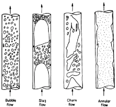
Figure 1.1: Gas-liquid flow patterns for vertical tubes as described by Taitel et al. (1980)10. .... 3
Figure 1.2: Pictures of an isolated Taylor bubble in a biphasic system. Image acquired with a moving camera and reproduced from the work of Campos and Guedes de Carvalho12. ... 4
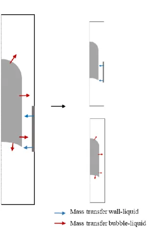
Figure 1.3: Schematic representation of the mass-transfer problems in study. ... 6
Figure 2.1: Schematic representation of the steps involved in a typical biofilm development process retrieved from the work presented by Stodley et al.15: 1) cell attachment; 2) adhesion; 3) and 4) maturation and 5) dispersion phases. Below the schematic representation, the growth of Pseudomonas aeruginosa under continuous-flow in a glass substratum is documented. ... 16 Figure 2.2: Flow patterns for a water-liquid system at 25ºC in a tube with a diameter of 5 cm (reprinted from Taitel et al.22) ... 17
Figure 2.3: Illustration of a Taylor bubble and the hydrodynamic regions normally present on the surrounding liquid flow. ... 19 Figure 2.4: Illustration of typical streamlines in the different slug flow sub-categories in milli/micro channels. ... 26 Figure 2.5: Illustration of the two-film model in a gas-liquid system: A) mass transfer resistance in both liquid and gas phase; B) mass transfer resistance only in the liquid phase (the gas phase is a pure gas). ... 38
Figure 3.1: Illustration of the flow regions and main hydrodynamic features involved in the rise of a Taylor bubble (adapted from Araújo et al., 2012)19. ... 58
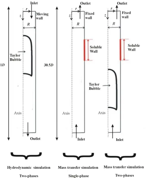
Figure 3.2: Representation of the domain and boundary conditions types for the systems established in each stage of the study. ... 61 Figure 3.3: a- Numerical dimensionless wall shear stress for different liquid velocities in the presence of a bubble with 2.2D of length; b- Numerical dimensionless wall shear stress in the presence of bubbles of different length (u=5.0x10⁻² m/s). z
n is the bubble nose position. ... 68
Figure 3.4: Representation of grid_2 in an axial slice. ... 68 Figure 3.5: a-Dimensionless concentration radial profiles for different meshes in the soluble region; b-Local mass transfer coefficients along the soluble wall for different meshes (z0 is the
soluble plate onset). The system concerned on this figure has a soluble plate of 0.25D and a u=1.0x10⁻¹ m/s. ... 70
xv
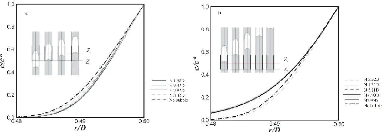
Figure 3.6: a-Local mass transfer coefficients for systems with different velocities and lengths of the soluble wall; b-Average mass transfer coefficients acquired numerically (squares) and through equations 3.12 and 3.13(lines)... 71 Figure 3.7: Normalized radial profiles taken at the middle of the soluble wall (zi) for a bubble
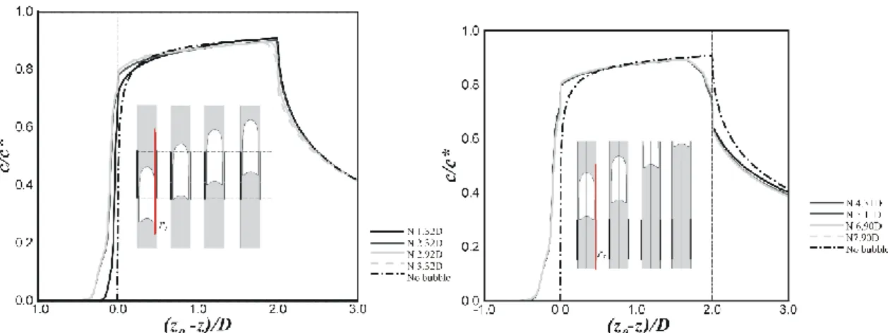
with a length of 2.2D in a system with u=5.0x10⁻² m/s: a-during bubble passage and b-after bubble passage. The dotted line represents the concentration profile in single phase flow. In the zoom, the relative position between the bubble and the middle plane is sketched (the darker line represents the soluble wall and the red line the middle plane of the soluble wall). ... 73 Figure 3.8: Axial normalized concentration profiles obtained at the radial position ri =0.499 D
(in red in the figure) for a bubble with a length of 2.2 D and with u=5.0x10⁻² m/s: a-during bubble passage and b-after bubble passage. The soluble plate is delimited by the vertical lines. The relative position between the bubble and the soluble wall is also sketched (the darker line represents the soluble wall). ... 74 Figure 3.9: Axial normalized concentration profiles before (a) and after (b, bubble at N 6.90D) the passage of the bubble in the soluble wall region for different radial positions; (c) axial normalized concentration profiles at ri = 0.4 D for different positions of the bubble during its rise.
The lines named “out” represent moments when the bubble nose is outside the domain considered. The soluble wall is delimited by the vertical dotted lines. The bubble had a length of 2.2D and the liquid velocity was 5.0x10⁻² m/s. ... 74
Figure 3.10: Axial normalized concentration profiles at the radial position ri =0.499 D for a
bubble with a length of 2.2D and different liquid velocities. The soluble plate is delimited by the vertical lines. ... 75 Figure 3.11:Axial normalized concentration profiles before (a) and after the passage of the bubble-tail at 4D from soluble plate (b) in the soluble wall region for different radial positions. The soluble wall is delimited by the vertical dotted lines. Bubble with a length of 2.2D flowing in a system with u=2.5x10⁻⁴ m/s, next to each graph there is the representation of the iso-surface
r=0.48D but for two velocities (u=2.5x10⁻⁴ m/s and u=5.0x10⁻² m/s). ... 76
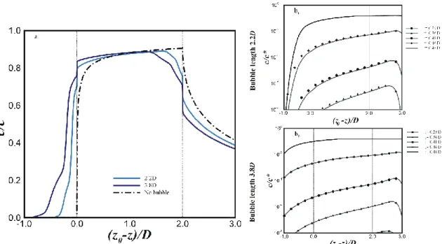
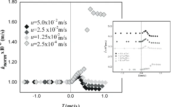
Figure 3.12:a- Normalized axial concentration profiles taken at r=0.499 D for bubbles with different lengths (2.2D and 3.8D) in a system with u=5.0x10⁻² m/s. The tail of the bubbles is at 3.8D. b- Axial normalized concentration profiles taken at different radial positions for bubbles with different lengths and the tail at 3.8D: b1-2.2D bubble length; b2-3.8D bubble length. The vertical dotted lines delimited the soluble wall. The c/c* scales used in part a and b are different (a-linear, b- logarithmic). ... 77 Figure 3.13: Evolution of the average mass transfer coefficient with time, as the bubble rises along a 2D soluble wall for a 2.2D bubble in a system with u=5.0x10⁻² m/s. Time 0 represents the instant the bubble reaches the soluble wall. The dotted line identifies the mass transfer coefficient for the same system without bubble flow. On the zoom inside the graph, representation of mass
xvi
transfer coefficient for a larger period of time is also present. On the right, local mass transfer coefficient at different moments, as the bubble rises along the soluble wall, are plotted for the same system. ... 78 Figure 3.14: Concentration fields obtained at the beginning of the soluble wall for different instants – before (0 s), during (2.8 s) and after (3.4, 100, 200, 300 s) the bubble flows through the soluble section. The bubble length is 2.2D and u=5.0x10⁻² m/s. ... 79
Figure 3.15: Concentration fields at the end of the soluble wall for different moments in a system with a u of 2.5x10⁻⁴ m/s and a bubble with a length of 2.2 D. ... 79 Figure 3.16: Average mass transfer coefficient at different moments, as the bubble rises along the soluble wall, for a 2.2D bubble in a system with u=2.5x10⁻⁴ m/s. Time 0 represents the instant the bubble reaches the soluble wall. The dotted line represents the mass transfer coefficient for the same system but without bubble flow. ... 80 Figure 3.17: Normalized average mass transfer coefficients against time. The bubble has a length of 2.2D and rises along the tube with different co-current liquid velocities. Time 0 represents the instant when the bubble reaches the soluble plate. On the right side, the raw average coefficients are plotted against time for the same systems. The mass transfer coefficient is represented for the same systems but without the bubble presence (lines). ... 81 Figure 3.18: Radial normalized concentration profiles when the bubble 2.2D reaches the end of the soluble wall on a system with u=5.0x10⁻² m/s. The dotted lines represent the profiles for the same positions in the absence of bubble. ... 83 Figure 3.19: Radial normalized concentration profiles along the developed film of a bubble with a length of 3.8D and a u=5.0x10⁻² m/s. Radial normalized velocity profiles for the same iso-surfaces are also plotted (lower graph). A sketch of the bubble position relatively to the wall, as well as the iso-surfaces chosen, is represented on the right side of the figure. ... 85 Figure 3.20: a-Streamlines in the wake region for a bubble with a Nf= 357; b-Normalized solute concentration inside the closed wake before (b1) and after (b2) its passage along the soluble plate. The bubble and wake position are also sketched. This representation was made for a system with a 2.2D bubble and u=5.0x10⁻² m/s. ... 86
Figure 3.21: Radial normalized concentration profiles near the wall for three axial positions on the wake region for a bubble with a 2.2D length and u=5.0x10⁻² m/s. On the left, it is sketched the wake positon relatively to the soluble wall. The dotted lines represent the concentration profiles before the bubble passage. ... 87
Figure 4.1: a) Schematic representation of the interface determination; b) Schematic representation of the interface cells and of Δx calculation based on the work of Özkan et al.54 . ... 115
xvii
Figure 4.2: Radial dimensionless concentration profiles at two different axial locations (each represented by the red line on the figure scheme of each plot), acquired with different mesh densities. Below, the figure represents the concentration distribution inside the mass boundary layer along the liquid film and the chosen mesh (100x3000 cells). The concentration (δc) and the
hydrodynamic (δh) boundary-layer thicknesses are represented for the system where U̅𝐿=0.025
m.s-1 (M=5.3x10⁻⁵, Sc= 1.84x10⁴ and Re
B=108). ... 116
Figure 4.3: Representation of the concentration contours in the nose, film and tail regions for different moments until reaching a pseudo stationary-state. The results were obtained for a system with UL=0.025m.s-1 and a bubble length of 2.01D. An image with the streamlines around the bubble is also shown (M=5.3x10⁻⁵, Sc= 1.84x10⁴ and Re
B=108). ... 118
Figure 4.4: A) Dimensionless oxygen concentration in the liquid along the axial direction for three radial positions (z0 corresponds to the axial coordinate of the bubble nose tip). B) Dimensionless concentration of oxygen along streamlines around the bubble. The coordinate s along the streamlines starts at the I.P. plan (see representation in the right side). These numerical results correspond to a physical time of 1.5 s with U̅𝐿=0.025 m.s-1 and a bubble with 2.01D
(M=5.3x10⁻⁵, Sc= 1.84x10⁴ and Re
B=108). ... 119
Figure 4.5: Dimensionless concentration of oxygen along h (distance from the bubble surface along the normal direction) for different positions around the bubble nose. A grey region limited by the line that corresponds to 1% of the saturation concentration (dashed line) and the interface (full line) is represented. This simulation has run for 0.5 s with U̅𝐿=0.025 m.s-1 and a bubble with
2.01D (M=5.3x10⁻⁵, Sc= 1.84x10⁴ and Re
B=108). ... 120
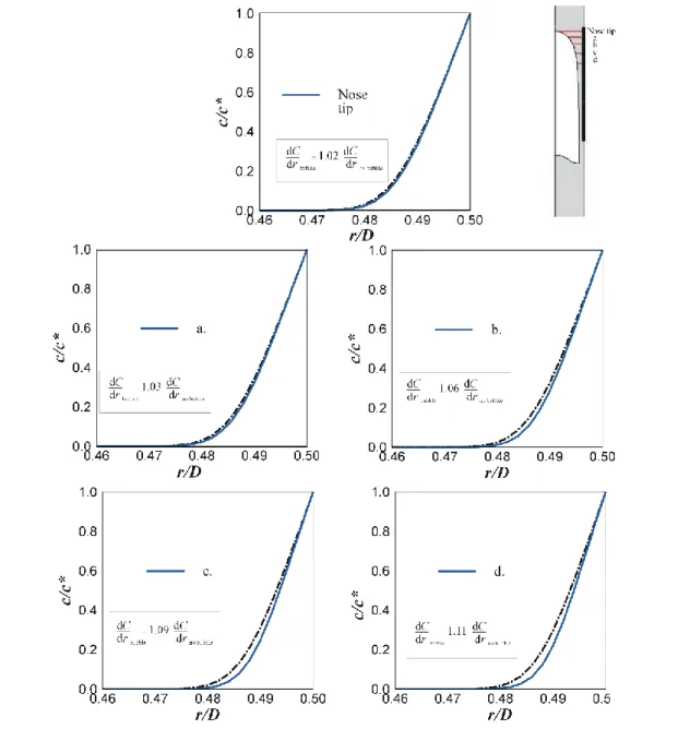
Figure 4.6: Dimensionless concentration of oxygen in the developed film region. The abscissas axis represents h (distance along the normal to the bubble surface), for different positions on the bubble film, normalized by the film thickness (δh). The corresponding axial positions as well as the line that represents 1% of the saturation concentration are schematically illustrated at the right side of the figure. This simulation has run for 0.3 s with U̅𝐿=0.050 m.s-1 and a bubble with 5.5D
(M=5.3x10⁻⁵, Sc=1.84x10⁴ and Re
B=133). A zoom for three different regions along the concentration profiles is represented in the lower part of the figure. ... 121 Figure 4.7: Local mass transfer coefficients along the bubble surface. Larger spheres indicate higher mass transfer coefficients. This simulation has run for 0.2 s with U̅𝐿=0.050 m.s-1 and a
bubble with a length of 3.5D (M=5.3x10⁻⁵, Sc= 1.84x10⁴ and Re
B=133). ... 122
Figure 4.8: Local mass transfer coefficients along the film region obtained for different velocities and bubbles with different lengths. For U̅𝐿=0.05 m.s-1 (A), the bubbles have a length of 2.1D (1),
3.5D (2), 5.5D (3) and 8.9D (4). For U̅𝐿=0.10 m.s-1 (B), the shorter bubble has a length of 2.1D
xviii
Figure 4.9: Local mass transfer coefficients along the bubble surface for different velocities. The dotted lines represent the global mass transfer coefficients. Next to each plot, a schematic representation of some positions is presented to help the interpretation of the plots (M=5.3x10⁻⁵, Sc= 1.84x10⁴). ... 125
Figure 4.10: Average Sherwood number for different bubble regions in function of the bubble Reynolds number (for M=5.3x10⁻⁵, Sc= 1.84x10⁴). The dashed lines represent the fitted equations for each zone. ... 126 Figure 4.11: Dimensionless concentration of oxygen in the developed film region acquired by simulation (Numerical). The dotted lines represent the profiles that would produce the mass transfer coefficients values estimated by the penetration (red line) and by the film (black line) theories. The abscissas axis represents h (distance along the normal to the bubble surface) normalized by the film thickness (M=5.3x10⁻⁵, Sc= 1.84x10⁴). ... 127
Figure 5.1: Flow patterns for milli/micro-channels based on the work of Rocha et. al23. The wall shear stress axial evolution obtained in the present work is also represented for each flow condition. ... 144 Figure 5.2: Schematic representation of the domain and boundary conditions. ... 146 Figure 5.3: Radial dimensionless concentration profiles for three positions along the soluble wall obtained for the different meshes considered in the density test. ... 150 Figure 5.4: Streamlines on the bubble surroundings (in a MFR) for ReB =10 and CaB =2.0.... 152
Figure 5.5: 1) Wall shear stress along the soluble wall for different instants during the bubble passage; 2) Radial profiles of the axial velocity component for three locations (A, B, C) along the Taylor bubble. A set of streamlines near the wall are represented on the left side of the bubble. ... 153 Figure 5.6: Axial normalized concentration profiles for a radial position near the wall (line in red in the sketch at the right side of the plot (ri=0.98D)). A schematic representation of the bubble position for each profile is also presented (top right). Plot A is a zoom in the pre-soluble wall region to better visualize the results (bottom right). ... 154 Figure 5.7: Radial normalized concentration profiles at the middle of the soluble wall for different instants of the bubble passage. A schematic representation to visualize the different bubble positions is also given – zw sets the beginning of the soluble wall and zi is the middle position
under consideration in this figure. ... 155 Figure 5.8: Average mass transfer coefficients along the soluble wall during the bubble passage (left side). The coordinate (zw-z0)/D represents the distance of the bubble nose from the starting
point of the soluble wall. Local mass transfer coefficients as a function of the distance to the beginning of the soluble plate, (zw-z)/D, (right side). The average coefficients for these specific
xix
Figure 5.9: Dimensionless concentration contours at the end of the soluble wall obtained for Case A (ReB =10 and CaB=1). Results are shown for three instants of the bubble passage. The thickness value of the boundary layer that corresponds to 10% of the solubility is also presented (𝛿10%).
... 157 Figure 5.10: Dimensionless concentration contours at the inception of the soluble wall obtained for Case A (ReB =10 and CaB=1). Results are shown for three instants: before, during and after the bubble passage. ... 157 Figure 5.11: Streamlines around the bubble in a MFR for a ReB =100 and CaB =0.8. ... 158
Figure 5.12: 1) Wall shear stress along the soluble wall for different instants during the bubble passage; 2) Radial profiles of the axial velocity component for four locations (A, B, C, D) along the Taylor bubble. The streamlines near wall are represented on the left side of the bubble. .. 158 Figure 5.13: Axial dimensionless concentration profiles for a radial position near the wall (red line in the sketch at the right side of the plot (ri=0.98D)). A schematic representation of the bubble position for each profile is also presented. Plot A is a zoom performed on the pre-soluble region of the wall. ... 159 Figure 5.14: Radial dimensionless concentration profiles on the middle of the soluble wall taken at different instants of the bubble passage. The schematic representation of the bubble position is also presented – the soluble plate beginning (zw) and the considered position (zi) are marked. 160
Figure 5.15: Concentration contours during the passage of the closed wake in the region enclosed by the soluble wall (ReB=100 and CaB=0.8). ... 160
Figure 5.16: Average mass transfer coefficients along the soluble wall (left side). The coordinate (zw-z0)/D represents the distance of the bubble nose to the starting of the soluble wall. Local mass
transfer coefficients as a function of the distance to the beginning of the soluble plate, (zw-z)/D,
(right side). The average coefficients for these specific moments are marked by red boxes placed along the curve of the left side plot. ... 161 Figure 5.17: Streamlines around the bubble in a MFR for ReB =0.1 and CaB =0.03... 162
Figure 5.18: 1) Wall shear stress along the soluble wall for different instants during the bubble passage; 2) Radial profiles of the axial velocity component for three locations (A, B, C) along the Taylor bubble. ... 162 Figure 5. 19: Dimensionless concentration contours for different instants during the bubble passage in the soluble wall region. ... 163 Figure 5.20: Axial dimensionless concentration profiles for a radial position near the wall (red line in the sketch of the right side of the plot (ri=0.98D)). A schematic representation of bubble position for each profile is also presented. Plot A is a zoom performed on the pre-soluble region of the wall. ... 164 Figure 5.21: Radial dimensionless concentration profiles on the middle of the soluble wall for a sequence of moments during the bubble passage. The schematic representation of the bubble
xx
position is also presented – the soluble plate beginning (zw) and the considered position (zi) are
marked. ... 165 Figure 5.22: Average mass transfer coefficients along the soluble wall. The coordinate (zw-z0)/D
represents the distance of the bubble nose to the starting of the soluble wall. Local mass transfer coefficients as a function of the distance to the beginning of the soluble plate, (zw-z)/D, (right
side). The average coefficients for these specific moments are marked by red boxes placed along the curve of the left side plot. ... 166
Figure 6.1: Different flow characteristics for slug flow regime in milli/micro-channels based on the work of Rocha et. al26. ... 182
Figure 6.2: Variation of the film thickness with the Capillary number accordingly to equation (4) – solid line. The film thicknesses of the chosen study-cases, numerically solved in the present work, are represented by the dots. Illustrations of the hydrodynamics representative of the different flow cases are also illustrated. ... 183 Figure 6.3: Average axial velocity in the developed film for the representative cases studied by Rocha et al.26 ... 184
Figure 6.4: Illustration of the domain and boundary conditions used for the system in study. 189 Figure 6.5: a) Schematic representation of the interface determination; b) Schematic representation of the interface cells and the Δx calculation based on the work of Özkan and coworkers46. ... 192
Figure 6.6: Radial concentration profiles for an axial position in the developed film region (left graph) and axial velocity profiles for a radial position at the middle of the liquid film (right graph). The profiles concern results obtained with different mesh densities for Case A1 (ReB=10 and CaB=2). ... 193
Figure 6.7: Concentration distribution inside the mass boundary layer along liquid film for ReB=10 and CaB=0.03. The symbol δc corresponds to the mass boundary layer thickness and δh to
the hydrodynamic film thickness. ... 194 Figure 6.8: Concentration contours and streamlines for three distinct hydrodynamic behaviors expected for slug flow in micro-channels. ... 195 Figure 6.9: Stationary concentration contours and streamlines (MFR) around the nose region for cases A1, B1 and C1. ... 196 Figure 6.10: Concentration contours and streamlines (MFR) around the tail for cases A1, B1 and C1. ... 196 Figure 6.11: Dimensionless axial velocity profiles below the bubble bottom (0.05D below the tip of the tail) for cases A1 and C1. The average liquid velocity (𝑼̅𝑳) was used as the reference value.
xxi
Figure 6.12: Concentration profiles for cases A1, B1 and C1 along the streamlines (s). Next to each plot, the location of the streamlines is also shown. ... 198 Figure 6.13: Axial concentration profiles for three positions between the interface and the tube wall for cases A1, B1 and C1. The positions are referenced to the film thickness (δh) where 0δh
corresponds to the bubble surface and 1δh to the tube wall. ... 199
Figure 6.14: Radial concentration profiles for different axial positions in the liquid ahead and below the bubble. The black lines represent the numerical results for Case A1, blue lines to case B1 and gray lines to Case C1. ... 200 Figure 6.15: Concentration profiles along the normal to the interface in the nose region: Cases A1 (upper left), B1 (upper right) and C1 (lower). A schematic representation of the different positions is presented. For each representation, a grey region limited by the line that represents 1% of the saturation concentration (dashed line) and the interface (full line) is added. ... 201 Figure 6.16: Concentration profiles along the normal to the interface in the film region: Case A1 (upper left), B1 (upper right) and C1 (lower). A schematic representation of the different positions is presented. For each representation, a grey region limited by the line that represents 1% of the saturation concentration (dashed line) and the interface (full line) is added. ... 202 Figure 6.17: Concentration profiles along the normal to the interface in the tail region: Case A1 (upper left), B1(upper right) and C1 (lower). A schematic representation of the different positions is presented. For each representation, a grey region limited by the line that represents 1% of the saturation concentration (dashed line) and the interface (full line) is added. ... 203 Figure 6.18: Qualitative representation of the local mass transfer coefficients obtained for cases A1, B1 and C1. Larger spheres correspond to higher mass transfer coefficients; a reference sphere is added to each representation. ... 204 Figure 6.19: Numerical results of the local mass transfer coefficients along the bubble surface: Case A1 (upper left), B1 (upper right) and C1 (lower). Next to each graph, a schematic representation of several positions along the bubble surface is added to better identify the corresponding coefficients. ... 205 Figure 6.20: Concentration fields around a bubble with a CaB of 2.0 (Case A). The streamlines are also represented on the liquid phase. ... 207 Figure 6.21: Concentration fields around a bubble with a CaB of 0.03 (Case C). The streamlines are also represented on the liquid phase. ... 208
xxii
List of Tables
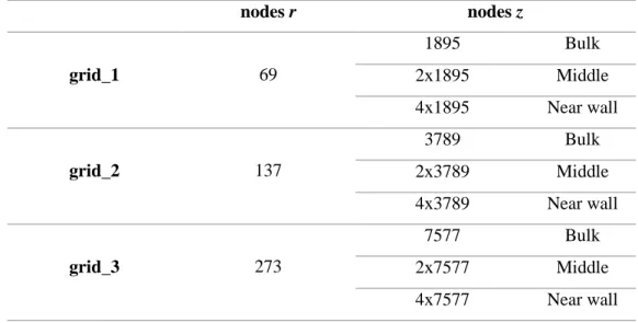
Table 3.1: Compilation of the conditions applied in the simulations for mass transfer from the soluble wall to the monophasic bulk fluid... 65 Table 3.2: Number of nodes for the different meshes considered in the mesh tests. ... 69 Table 3.3: Mass of solute before (initial) and after bubble passage (final) in different tube zones, for different simulated systems. The last column presents the total increase of mass on the system due to the bubble passage. ... 82 Table 3.4: Average mass transfer coefficients for the different zones around the bubble and the deviation to the mass transfer coefficient without bubble. ... 88 Table 3.5: Average mass transfer coefficients for the film and wake region acquired through equation 3.16 and 3.18 (corr) and by CFD simulation. ... 90
Table 4.1: Average liquid velocity, bubble velocity, bubble length and ReB used to study mass transfer phenomena. ... 111
Table 5.1: Number of nodes used in the meshes considered for the density test. ... 149 Table 5.2: Sherwood numbers determined from the simulations of monophasic systems and corresponding values estimated by Equations 5.15 and 5.16. ... 151 Table 5.3: Numerical average mass-transfer coefficients at the nose, film and tail regions. The corresponding deviations from the mass transfer coefficients for single phase flow (𝑘̅𝑚𝑝) are also
presented. ... 167 Table 5.4: Sherwood numbers from correlations and from numerical data associated to the bubble passage. ... 168 Table 5.5: Variation of mass transferred in different zones, for cases A, B and C. ... 169
Table 6.1: Number of nodes used in the mesh independence tests. ... 193 Table 6.2: Average mass transfer coefficients for the whole bubble (𝑘total ), nose (𝑘𝑛 ), film (𝑘𝑓 ) and tail (𝑘𝑡 ) regions. ... 206 Table 6.3: Identification of the simulated systems regarding the main dimensionless numbers. ... 207 Table 6.4: Average global mass transfer coefficients for systems with different Reynolds numbers. ... 209 Table 6.5: Global mass transfer coefficients estimated by the correlations available in literature and by numerical simulations. ... 210
1 Chapter 1 – Introduction
Chapter 1
3 1.1 Relevance and motivation
Mass transfer is one of the most important phenomena occurring in natural and industrial processes. It is essential to describe biological processes like respiration1,2 or the nutrient transport3. For industrial applications, mass transfer is needed to describe the mechanisms in most of the current operating units, and, in particular, when focus is placed on environmental aspects. Chemical reactors responsible for wastewater treatment4,5 and the development of clean energies as fuel cells6,7 are some of the most relevant examples.
The thematic of mass transfer in two-phase flow systems has a huge importance and complexity. Mass transfer in gas-liquid two phase flows can be affected by, among other factors8,9, the physical properties of the fluids involved, geometry and dimensions of the channels/devices and the type of flow pattern. In its turn, the nature of the flow pattern can be influenced by the gas and liquid flow rates, properties of the liquid and even channel configuration.
Figure 1.1: Gas-liquid flow patterns for vertical tubes as described by Taitel et al. (1980)10.
From all of the major gas-liquid flow patterns identified in Figure 1.1, slug flow is one of those that attracts more attention to research, due to its common occurrence in several industrial and natural processes. Perfect examples are the transport of hydrocarbons, geothermal power plants to produce steam, water cooling of nuclear reactors, and enhancement of heat and mass transfer in fluidized chemical reactors11. Slug flow is mainly characterized by the presence of large gaseous bubbles separated by liquid slugs (see Figure 1.2). These bubbles are commonly known as Taylor bubbles.
4
Figure 1.2: Pictures of an isolated Taylor bubble in a biphasic system. Image acquired with a moving camera and reproduced from the work of Campos and Guedes de Carvalho12.
The particular hydrodynamic characteristics of slug flow can also be explored to promote mass and heat transfer enhancement, namely, through the presence of long bubbles followed by liquid slugs where mixing can reduce the mass and heat transfer resistances13.
A standard and relevant application of slug flow involving mass transfer phenomena is the cleaning of the surfaces of separation membranes. The use of membranes in purification processes has as a major setback – membrane fouling. Membranes can be cleaned with the help of chemical products, however, this method may impair the membrane selectivity and reduce its lifetime or even produce undesirable secondary products14. Several studies have evaluated the effect of slug flow in order to minimize membrane fouling13,15–19. The flow of Taylor bubbles promotes the displacement of the concentration polarization layer and induces rapid and abrupt variations on the wall shear stress which, in turn, will prevent the settling of particles at the membrane surface17,19. The work of Cabassad20 claims an increase of 60-110% on the permeated flux associated to the slug flow passage, which is a very good indicator.
Based on similar principles applied to membranes, another potential scenario of mass transfer enhancement is the cleaning of medical devices. Medical devices embrace a wide range of dimensions, however, several of them have channels with diameters below 100 μm21. These micro devices are continuously in contact with microorganisms that can adhere to their walls and, eventually, it will lead to the formation of biofilms. The presence of biofilms cause, most of the times, the obstruction or clogging of the device but, more importantly, it can offer an easier way for pathogenic agents to develop and become a source of hospital-acquired infections. As a reference to understand the magnitude of this problem, in England, during the year of 2006, around 8.2% of the patients contracted an infection as a result of a healthcare treatment22. This value was reduced to 6.4% after the implementation of several guidelines for a good practice dealing with medical devices.23 Furthermore, in the United States, 65% of hospital-acquired
5
infections are due to biofilms and this is the fourth leading cause of death24,25. Infections stemming from medical devices increase morbidity and mortality and they also cause a huge financial burden26,27. In Europe, it led to extra 16 million days of hospital stay and about 30 000 attributable deaths, leading to annual cost around 7 billion euros. While in the USA, in 2004, it led to costs around 6.5 billion dollars28.
The cleaning of medical devices based on the use of detergents with surfactant and without enzymes has proven itself to be ineffective29. Additionally, some disinfectants are not completely successful on cleaning these devices and can also impair other procedures, e.g., it can affect the material of the device when combined with the use of bleach containing sodium hypochlorite29. From a proactive perspective, the most effective way of preventing biofilms development is to avoid/control the bacterial adhesion to the wall surface. A potentially simple and efficient way to achieve this is by the continuous passage of micro bubbles through the devices during a specific period of time and independently of the device use. Besides the preventive role on avoiding biofilm formation, the presence of Taylor bubbles can also help controlling the biofilm growth after its development. The current lack of knowledge necessary to fully understand and enhance the efficiency of this kind of cleaning process is the main driving force behind the present work. More specifically, important research gaps were identified regarding the mass transfer processes that may govern this process: a) from the soluble matter attached to the wall to the flowing liquid in the vicinity of a Taylor bubble; and b) from a Taylor bubble composed by a soluble component to the flowing liquid for a possible posterior reaction with the soluble matter detached from the wall –Figure 1.3.
6
Figure 1.3: Schematic representation of the mass-transfer problems in study.
In a simplified manner, mass transfer can be defined as the transport of a substance through another. It is commonly known that the fundamentals of mass transfer mechanisms are directly linked to the hydrodynamics of the system9. As aforementioned, the movement of a Taylor bubble is responsible for a drastic change on the hydrodynamic characteristics of the surrounding liquid flow. So, in this work, a detailed numerical study was performed to evaluate the impact of an individual Taylor bubble in the mass transfer rates of the previously illustrated processes/steps (Figure 1.3). Furthermore, since the ratios between the governing forces in macro and micro-scales differ considerably, another important motivation was to perform the referred evaluation at both scales. It is also relevant notice that, such a systematic study about mass transfer in both macro and micro-scales is still not understood in the literature.
Among other possible applications, the knowledge acquired from this work will be a first step to prove the potential of using slug flow (i.e., a continuous sequence of Taylor bubbles) to clean medical devices and prevent biofilm formation. Due to the relevancy of this practical scenario, the success of the present study is expected to have a mid-term real impact in our society and daily life.
7 1.2 Objectives
In this work, a study on mass transfer for slug flow regime is presented. The main technical goal was to establish numerical procedures to solve simultaneously mass transfer and hydrodynamic fields, for macro and micro-scales, supported on the accuracy of computational fluid dynamics (CFD) techniques. The pursuit of this goal has undergone detailed fundamental studies that were planned following a set of successive steps and intermediate objectives for two main scenarios:
Mass transfer from a soluble wall to a flowing liquid:
o validation of a simulation method able to predict the transport of species from a wall to a surrounding liquid phase. This task concerned systems comprising the absence (single-phase flow) and presence of a rising individual Taylor bubble (gas-liquid flow);
o post-processing and interpretation of the numerical results based on the fundamentals of mass transfer mechanisms. Estimation of local and average mass transfer coefficients, as well as analyzing the effect of the different hydrodynamic regions that surround a Taylor bubble on the referred mechanisms;
o overall quantification of the solute transferred from the wall in single-phase and slug flow systems to assess the potential for enhancement;
Mass transfer from a soluble Taylor bubble to the surrounding liquid:
o validation of a simulation method to solve the transfer of species between a pure and soluble rising Taylor bubble and the co-currently flowing liquid;
o analyzing the numerical results of the previous point to produce reliable data of gas-liquid mass transfer coefficients. Study the effect of different parameters (velocity and bubble length) and of the bubble regions on the levels of the referred gas-liquid mass transfer;
o overall quantification of the mass transferred between the soluble bubble and the flowing liquid.
The sequence of steps/objectives listed above was addressed first for macro-scale scenarios and, in a second stage of this work, were reproduced for micro-scale systems. All the studies were performed in laminar flow regime conditions in the liquid phase.
8 1.3 Outline
After the general framework provided in this first chapter, a deeper insight on the current state of the art regarding the subjects involved in this thesis is presented in Chapter 2. The detailed description of the methodologies applied and developed, main results gathered throughout the work and corresponding discussions can be found in the subsequent chapters. These chapters (from 3 to 6) are based on papers published or under review in peer-reviewed international journals:
Chapter 3: Mass transfer from a soluble wall to the flowing liquid around a bubble in a macro-scale system (published in AIChE Journal) with the tittle “CFD Studies Coupling Hydrodynamics and Solid-Liquid Mass Transfer in Slug Flow for Matter Removal from Tube Walls”;
Chapter 4: Mass transfer from a soluble bubble to the flowing liquid around in a macro-scale system (under review in Chemical Engineering Research and Design) with the tittle “Mass Transfer of a soluble compound from a Taylor bubble to the surrounding liquid – A Numerical Approach”;
Chapter 5: Mass transfer from a soluble wall to the flowing liquid around a bubble in a micro-scale system (under review in International Journal of Heat and Mass Transfer) with the tittle “Mass transfer from a soluble wall into gas-liquid slug flow in a capillary tube”;
Chapter 6: Mass transfer from a soluble bubble to the liquid flowing around in a micro-scale system (under review in Microfluidics and Nanofluidics) with the tittle “Mass Transfer from a Taylor bubble to the surrounding liquid in micro-scale – A Numerical Approach”
In chapter 3, a CFD study on the mass transfer between a finite soluble wall and the flowing liquid under the presence of an individual Taylor bubble is presented. A detailed analysis of the evolution of the solute concentration distribution due to the bubble passage is discussed. Local and average mass transfer coefficients were determined and the latter were compared with the values present in the literature. The following chapter (Chapter 4) addresses the transport of mass between a soluble Taylor bubble of pure oxygen to the surrounding liquid in co-current flow configuration (laminar regime in the flowing liquid). This work shows the effect of the bubble different hydrodynamic regions (nose, film and tail) on the mass transfer. The acquired values for average mass transfer coefficients are compared to values available in the literature, however this comparison highlighted the lack of appropriated correlations to predict the mass transfer in the conditions studied. These two studies were performed for conventional scales and allowed to
9
achieve a global understanding of the nuances involved in the corresponding mass transfer mechanisms. Furthermore, the success of the referred macro-scale studies was supported on the establishment of appropriate methods to simulate and post-process numerical results regarding mass transfer in two-phase flow. The development of this important “know-how” was essential and could be transposed to similar systems in micro-scales. As a logical consequence, the studies comprised in Chapters 5 and 6 were elaborated in a similar way as the ones presented in Chapters 3 and 4, respectively, but now regarding mass transfer in micro-scale slug flow systems. The detailed behavior of the distribution of solute concentration was numerically obtained for different flow conditions and, based on this data, the corresponding mass transfer coefficients were determined.
Finally, Chapter 7 encloses this thesis with the overall conclusions taken from all the work developed and some suggestions for future research.
Literature Cited
1. Yeh H-C. Use of a heat transfer analogy for a mathematical model of respiratory tract deposition. Bull Math Biol. 1974;36:105-116. doi:10.1016/S0092-8240(74)80014-5. 2. Condorelli P, George SC. Theoretical Gas Phase Mass Transfer Coefficients for
Endogenous Gases in the Lungs. Ann Biomed Eng. 1999;27(3):326-339. doi:10.1114/1.145.
3. Tharakan A, Norton IT, Fryer PJ, Bakalis S. Mass Transfer and Nutrient Absorption in a Simulated Model of Small Intestine. J Food Sci. 2010;75(6):E339-E346. doi:10.1111/j.1750-3841.2010.01659.x.
4. Cockx A, Do-Quang Z, Audic J., Liné A, Roustan M. Global and local mass transfer coefficients in waste water treatment process by computational fluid dynamics. Chem Eng Process Process Intensif. 2001;40(2):187-194. doi:10.1016/S0255-2701(00)00138-0. 5. Qi N, Zhang H, Jin B, Zhang K. CFD modelling of hydrodynamics and degradation
kinetics in an annular slurry photocatalytic reactor for wastewater treatment. Chem Eng J. 2011;172(1):84-95. doi:10.1016/j.cej.2011.05.068.
6. Hashemi F, Rowshanzamir S, Rezakazemi M. CFD simulation of PEM fuel cell performance: Effect of straight and serpentine flow fields. Math Comput Model. 2012;55:1540-1557. doi:10.1016/j.mcm.2011.10.047.
7. Zahi I, Rossi C, Faucheux V. Micro PEM fuel cell current collector design and optimization with CFD 3D modeling. Int J Hydrogen Energy. 2011;36:14562-14572. doi:10.1016/j.ijhydene.2011.08.020.
8. Sideman S, Hortaçsu Ö, Fulton JW. Mass Transfer in Gas-Liquid Contacting Systems. Ind Eng Chem. 1966;58(7):32-47. doi:10.1021/ie50679a006.
10
9. Treybal RER, Robert ET. Mass-Transfer Operations.; 1981. doi:10.1002/aic.690020430. 10. Taitel Y, Barnea D, Dukler AE. Modelling flow pattern transitions for steady upward
gas-liquid flow in vertical tubes. AIChE J. 1980;26:345-354. doi:10.1002/aic.690260304. 11. Fabre J, Line A. Modeling of Two-Phase Slug Flow. Annu Rev Fluid Mech.
1992;24(1):21-46. doi:10.1146/annurev.fl.24.010192.000321.
12. Campos JBLM, Guedes de Carvalho JRF. An experimental study of the wake of gas slugs rising in liquids. J Fluid Mech. 1988;196:27-37. doi:10.1017/S0022112088002599. 13. Bellara S, Cui Z, Pepper D. Gas sparging to enhance permeate flux in ultrafiltration using
hollow fibre membranes. J Memb Sci. 1996;121:175-184.
14. Liu C, Caothien S, Hayes J, Caothuy T, Otoyo T, Ogawa T. Membrane Chemical Cleaning : From Art to Science. Am Water Work Assoc. 2001:25.
15. Cui ZF, Wright KIT. Flux enhancements with gas sparging in downwards crossflow ultrafiltration : performance and mechanism. 1996;117:109-116.
16. Ghosh R, Cui ZF. Mass transfer in gas-sparged ultrafiltration: upward slug flow in tubular membranes. J Memb Sci. 1999;162(1-2):91-102. doi:10.1016/S0376-7388(99)00126-X. 17. Cabassud C, Laborie S, Lainé JM. How slug flow can improve ultrafiltration flux in
organic hollow fibres. J Memb Sci. 1997;128:93-101. doi:10.1016/S0376-7388(96)00316-X.
18. Li QY, Cui ZF, Pepper DS. Effect of bubble size and frequency on the permeate flux of gas sparged ultrafiltration with tubular membranes. 1997;67:71-75.
19. Cui ZF, Bellara SR, Homewood P. Airlift crossflow membrane filtration - A feasibility study with dextran ultrafiltration. J Memb Sci. 1997;128:83-91. doi:10.1016/S0376-7388(96)00280-3.
20. Laborie S, Cabassud C, Durand-Bourlier L, Laine JM. Characterisation of gas-liquid two-phase flow inside capillaries. Chem Eng Sci. 1999;54:5723-5735. doi:10.1016/S0009-2509(99)00146-3.
21. Ducheyne P, Grainger DW, Healy KE, Hutmacher DW, Kirkpatrick CJ (C. J. Comprehensive Biomaterials II.
22. National Audit Office. Reducing Healthcare Associated Infections in Hospitals in England. Natl Audit Off. 2009;(June):1-69.
23. Barnes L, Cooper IR, eds. Biomaterials and Medical Devices. Vol 58.; 2016. doi:10.1007/978-3-319-14845-8.
24. Wenzel RP, Edmond MB. The impact of hospital-acquired bloodstream infections. Emerg Infect Dis. 2001;7(2):174-177. doi:10.3201/eid0702.010203.
25. Bryers JD. Medical biofilms. Biotechnol Bioeng. 2008;100(1):1-18. doi:10.1002/bit.21838.
11 2008. doi:10.1007/978-3-540-75418-3.
27. Percival SL, Suleman L, Donelli G. Healthcare-Associated infections, medical devices and biofilms: Risk, tolerance and control. J Med Microbiol. 2015;64(4):323-334. doi:10.1099/jmm.0.000032.
28. Report on the Burden of Endemic Health Care-Associated Infection Worldwide Clean Care Is Safer Care.; 2011. www.who.int. Accessed August 3, 2018.
29. Merritt K, Hitchins VM, Brown SA. Safety and cleaning of medical materials and devices. J Biomed Mater Res. 2000;53(2):131-136. doi:10.1002/(SICI)1097-4636(2000)53:2<131::AID-JBM1>3.0.CO;2-I.
13
Chapter 2 – State of the art
Chapter 2
15
In order to fully understand the problem addressed in this work, a brief description on several topics will be presented in the following sections.
First, since the ultimate goal is to remove biofilms, a brief insight on the principal characteristics of these communities is given. Then, as a potential solution, we propose to control the biofilm growth by promoting the passage of Taylor bubbles - slug flow. This flow pattern presents a series of distinct characteristics that will be discussed for both macro and micro-scales, since important differences occur in the governing forces when the dimension range is changed. Afterwards, the methodologies used to solve this problem are introduced: the computational fluid dynamic (CFD) techniques. A general view on the software chosen as well as the steps necessary to successfully run a numerical study are presented. Finally, some mass transfer studies already available in the literature are also cited and discussed, in order to frame the work developed and highlight the main challenges of the current state of the art.
2.1 Biofilms
A biofilm is a set of microorganisms that co-exist in a cooperative community embedded in a matrix of extracellular polymeric substance (EPS) that can be attached to different substrata1. EPS is considered the primary matrix material of the biofilm and, in its structure, contains proteins, nucleic acids, lipids, cellular debris and polysaccharides. This structure helps to protect the microorganisms from the physical and antimicrobial agents. The sustainable growth of microorganisms in structured medium like biofilms increases their virulence, and also offers extra resistance to their removal by chemical and physical cleaning agents. The organisms present in a biofilm can induce diseases from single cells or aggregates that detach from the original structure and colonize other regions. Besides that, these communities may also produce endotoxins2–4. All biofilm communities are unique and heterogeneous and can be composed by different species. Several biofilm structures/types can be found in different conditions5. The dental biofilm is one of the most well studied5. It consists of a variety of microorganisms that present several physical, metabolic and molecular interactions6. The existence of a dental biofilm can contribute to healthy periodontium7. However, the presence of Streptococcus mutans or Porphyromonas gingivalis have been related with the appearance of dental caries and periodontal disease, indicating that the competition between beneficial and virulent bacteria will define the beneficial or prejudicial effect of the biofilm presence8.
Another relevant example regards Pseudomonas aeruginosa, which is an ubiquitous species present in soil and water9 that can form biofilms. It is classified as an opportunistic pathogen since it often colonizes immunocompromised patients and the lungs of cystic fibrosis patients10. It forms a mushroom-type structure when glucose is used as a carbon source, however, if citrate is used as carbon source, the biofilm develops as a flat but dynamic structure11.
16
The biofilm subpopulations will adapt themselves in order to provide the best tolerance to antimicrobial agents and to the alteration of environmental conditions12. It is important to note that, the complex and variable nature of biofilm structure and interactions are influenced by factors like the properties of the fluid (flow, velocity, temperature, proteins and nutrient levels), the cell properties (charge, hydrophobicity, and signaling molecules) and the material surface properties (roughness, hydrophobicity, chemical composition and charge).
Being a “living” community, the biofilm formation and maturation has several stages3,13–15. The first stage consists in the attachment of the microorganisms to a surface. The microorganisms can be transported to the surface by mass transfer processes like diffusion, convection or sedimentation16. This initial phase is reversible, and so, it presents itself as the ideal opportunity to interfere and prevent the formation of biofilms. After the initial interaction and attachment, the cells can adhere to the surface - adhesion. This phase is irreversible due to the binding by EPS. During this phase, bacteria start to multiply, while emitting chemical signals between them and thus forming cell aggregates. Afterwards, this structure will mature. In a final phase, some organisms can detach from the structure and colonize a new area13,15 – Figure 2.1.
Figure 2.1: Schematic representation of the steps involved in a typical biofilm development process retrieved from the work presented by Stodley et al.15: 1) cell attachment; 2) adhesion; 3) and 4) maturation
and 5) dispersion phases. Below the schematic representation, the growth of Pseudomonas aeruginosa under continuous-flow in a glass substratum is documented.
Biofilms can be beneficial in several situations like water treatment processes17,18. However, if not properly controlled, its presence can become problematic especially when it starts to affect the performance of devices or, in even more serious cases, it may lead to situations of public health concern. It is estimated that 65% of bacterial infections are caused by bacterial biofilms19. Regarding a particularly relevant field of occurrence, one of the first associations between biofilms and medical devices was described by Johanson et al.20. To cite a few problematic examples, the frequency of infections that occur within different medical devices has been