Structural optimization using the Finite Element Method

(1)

Universidade Católica Portuguesa

Faculdade de Engenharia

Universidade Católica Portuguesa

Faculdade de Engenharia

Modelo de Auditoria de Gestão do Risco Operacional

Aplicações no Contexto de Instituições Financeiras

Jose da Silva e Silva

Monografia

Mestrado em Engenharia Informática

Orientador: Prof. Doutor Easdffa Ffasfasf

Co-Orientadora: Doutora Gasfdasfasf Hafsffgtsdr5ter

Junho de 2012

Structural Optimization using the Finite Element Method

João Pedro Pires Mesquita

Dissertação para obtenção do Grau de Mestre em

Engenharia Civil

Júri

Prof. Doutor Manuel Barata Marques (Presidente)

Engº. Timo Prißler (Co-Orientador)

Prof. Doutor Mário Rui Tiago Arruda (Convidado)

(2)

(3)

i

LIST OF FIGURES

Figure 1-1 - Approximation methods that led to the FEM ... 2

Figure 2-1 - Problem’s domain, Dirichlet and Neumann boundaries ... 4

Figure 2-2 - Complementary energy density and its variation ... 8

Figure 2-3 - Internal energy density and its variation ... 8

Figure 2-4 - Rectangular plate ... 16

Figure 2-5 - Tension coupon ... 18

Figure 3-1 - Size optimization problem: ten-bar truss ... 23

Figure 3-2 - Shape optimization problem – Michell’s arch shape optimization ... 24

Figure 3-3 - Topology optimization problem: bicycle frame topology optimization... 24

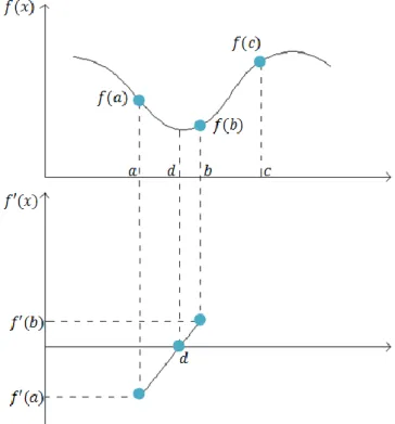
Figure 3-4 - Bracketing interval when f(d)>f(b) ... 27

Figure 3-5 - Bracketing interval when f(d)<f(b) ... 27

Figure 3-6 - Approximation of a function's minimum according to Brent's method ... 28

Figure 3-7 - Linear interpolation yields a new bracketing point (d) in the acceptable region of the bracketing interval ... 30

Figure 3-8 - Linear interpolation yields a new bracketing point (d) in the unacceptable region of the bracketing interval ... 30

Figure 3-9 - "Reflection" and “contraction” of the highest value point from the initial simplex in a valley simulated by the blue dashed lines ... 32

Figure 3-10 - General concepts of a linear programming problem ... 41

Figure 3-11 - Constant stress bar ... 43

Figure 3-12 - Function Vtot for a = 0 and c = 0.188 ... 46

Figure 3-13 - Function Vtot for b=0.0096 and c=0.188 ... 47

Figure 3-14 - Variation of the cross sectional radius – approximated and exact values ... 48

Figure 3-15 - Cantilever plate ... 51

Figure 3-16 – von Mises stress output of the non-optimized cantilever plate ... 53

Figure 3-17 – Deformed shape of the cantilever plate ... 54

Figure 3-18 - Different density elements in the model ... 55

(7)

v

Figure 3-20 - Smoothed structure topology design ... 56

Figure 3-21 - Stress output of the optimized cantilever plate ... 58

Figure 3-22 - Deformation of the optimized cantilever plate ... 59

Figure 4-1 - Front left view of the wheel carrier ... 62

Figure 4-2 - Front right view of the wheel carrier ... 62

Figure 4-3 - Back left view of the wheel carrier ... 63

Figure 4-4 - Back right view of the wheel carrier ... 63

Figure 4-5 - Pre/post-processor and solver used and respective main capabilities ... 65

Figure 4-6 - Load application points ... 66

Figure 4-7 - Constraint application points ... 66

Figure 4-8 - Maximum stress area for the Ratterkerb3 load case... 71

Figure 4-9 - Maximum stress area for the Ludwigskerb load case ... 71

Figure 4-10 – Maximum stress area for the Bremsen load case... 72

Figure 4-11 - Comparison between the stress values for the different averaging definitions for a mesh with dominant edge length of 3 mm ... 73

Figure 4-12 - Comparison between the stress values for the different averaging definitions for a mesh with dominant edge length of 4 mm ... 74

Figure 4-13 - Comparison between the stress values for the different averaging definitions for the mesh with dominant edge length of 5 mm ... 75

Figure 4-14 - Front view of the meshed structure ... 77

Figure 4-15 - Back view of the meshed structure ... 77

Figure 4-16 - Stress distribution for the Ratterkerb3 load case ... 79

Figure 4-17 - Stress distribution for the Ludwigskerb load case... 80

Figure 4-18 - Stress distribution for the Bremsen load case ... 81

Figure 4-19 - Deformed structure for the Ratterkerb3 load case... 83

Figure 4-20 - Maximum displacement area for the Ratterkerb3 load case ... 83

Figure 4-21 - Deformed structure for the Ludwigskerb load case ... 84

Figure 4-22 - Deformed structure for the Bremsen load case ... 85

Figure 4-23 - Maximum displacement area for the Bremsen load case ... 85

Figure 4-24 - Identification of the areas discarded from the optimization ... 87

(8)

vi

Figure 4-26 - Basic topology result for material reduction of 10% and threshold value of 0.0 .. 88

Figure 4-29 - Comparison between the non-optimized structure and the optimized model with a threshold value of 0.2 ... 92

Figure 4-32 - Front view of the optimized wheel carrier ... 96

Figure 4-33 - Front view of the optimized wheel carrier ... 96

Figure 4-34 - Back view of the optimized wheel carrier ... 97

Figure 4-35 - Back view of the optimized wheel carrier ... 97

Figure 4-36 – Areas requiring different optimization approaches ... 99

Figure 4-37 – Phases of the creation of the optimized structure (left side view) ... 100

Figure 4-38 – Phases of creation of the optimized structure (right side view) ... 101

Figure 4-39 - Stress output of the non-optimized and optimized structures for the Ratterkerb3 load case ... 106

Figure 4-40 - Displacement output of the non-optimized and optimized structures for the Ratterkerb3 load case ... 107

Figure 4-41 - Stress output of the non-optimized and optimized structures for the Ludwigskerb load case ... 109

Figure 4-42 - Displacement output of the non-optimized and optimized structures for the Ludwigskerb load case ... 110

Figure 4-43 - Stress output of the non-optimized and optimized structures for the Bremsen load case ... 112

Figure 4-44 - Maximum stress area for the Bremsen load case - optimized structure ... 113

Figure 4-45 - Maximum stress area for the Bremsen load case – non-optimized structure ... 113

Figure 4-46 - Maximum stress area in the optimized structure for the Bremsen load case ... 114

Figure 4-47 - Displacement output of the non-optimized and optimized structures for the Bremsen load case ... 115

(9)

vii

LIST OF TABLES

Table 1 - Dimensions and properties of the rectangular plate ... 16

Table 2 - Deformed shape and eigenfrequency corresponding to the first eigenmode for different element dimensions ... 17

Table 3 - Dimensions and properties of the tension coupon ... 19

Table 4 – von Mises stress diagram and maximum von Mises stress for increasing number of elements... 20

Table 5 - Bounds and restrictions of the problem ... 44

Table 6 - Cross sectional area of the bar – approximated and exact values ... 48

Table 7 - Dimensions and properties of the cantilever plate ... 51

Table 8 - Aluminum Al7075 properties ... 64

Table 9 - Applied loads for the Ratterkerb3 load case ... 67

Table 10 - Applied loads for the Ludwigskerb load case ... 67

Table 11 - Applied loads for the Bremsen load case ... 68

Table 12 - Maximum stress for the mesh with dominant edge length of 3 mm ... 73

Table 13 - Maximum stress for the mesh with dominant edge length of 4mm ... 74

Table 14 - Maximum stress for the mesh with dominant edge length of 5 mm ... 75

Table 15 - Maximum stress values in the non-optimized structure ... 78

Table 16 - Maximum displacement values in the non-optimized structure ... 82

Table 17 - Mass reduction obtained through optimization ... 95

Table 18 - Load cases created for the stiffness comparison between the optimized and non-optimized structures ... 103

Table 19 - Comparison between displacement values of the optimized and non-optimized structures for four load application points ... 104

(10)

(11)

ix

NOTATION

The symbols used in this work are defined upon the first occurrence in the text. However, for the reader’s convenience the meaning of the main acronyms and symbols are given here.

Abbreviations

FEM Finite Element Method DOF Degrees-of-freedom MPC Multiple Point Constrain

Symbols

Domain of a given physical problem Boundary of the domain

Dirichlet boundary Neumann boundary Displacement field External force Stress components Strain components Material stiffness matrix K Finite element stiffness matrix Body force field

Equilibrium (divergence) differential operator Compatibility (gradient) differential operator Displacements enforced on the Dirichlet boundary X Nodal displacement values

U Displacement approximation functions , Test functions

(12)

x Matrix of the outward normal (Chapter 2) or

Generic direction versor (Chapter 3)

Internal energy density

Variation of the internal energy density

Complementary energy density

Variation of the complementary energy density

Total internal energy

Total potential energy Work of the external forces

Initial state of deformation Complementary potential energy

Complementary internal energy

Work of the reactions on the enforced boundary displacements A generic linear differential operator

Eigenfrequency

E Young’s modulus

Poisson ratio Mass density

Maximum stress in a given body Stress concentration factor

The golden ratio Versors of directions i

P Arbitrary initial position vector The Hessian matrix

Approximation of the inverse of the Hessian matrix Relative density

(13)

(14)

xii

ABSTRACT

This work reports on the formulation of the conforming finite element method (FEM) and its application to structural optimization problems. The FEM is nowadays the most widely used technique for obtaining approximate solutions of complex engineering problems that cannot be solved analytically.

The conforming finite element formulation can be reached using several approaches. One of the most general strategies is based on the weak-form of the equations governing the problem. However, rather than a pure mathematical approach, it is often more appealing to the structural engineer to reach the finite element formulation through more physically-meaningful strategies, such as the virtual work or the variational principle forms of the problem. All three of these strategies are briefly presented.

One of the most important topics in the finite element theory is the quality of the solutions. The most commonly used method to increase the quality of a finite element solution is to increase of the number of elements used in the model (mesh refinement). In this work, two numerical examples are presented to illustrate the convergence of the finite element solutions under mesh refinement.

An important application of the FEM and the focus of this work is the structural optimization. The purpose of the structural optimization is to minimize (or maximize) an objective function while respecting certain restrictions. The extremum of a continuous function on a certain interval can either correspond to a point where the gradient is null, or it may lay on the boundary of the interval. Several numerical methods for identifying null gradient points of a function are described in this work. When the extremum of a function lays on the boundary of its interval of definition, an effective minimization method should ensure that the boundaries are searched in such a way that every new iteration yields a result closer to the extremum than the one before. The basic aspects of the constrained minimization methods are briefly presented here and applied to two structural optimization problems, namely the size optimization of a bar subjected to its own weight and the topology optimization of a cantilever plate subjected to a concentrated load applied to its tip.

A large scale practical example of structural optimization, consisting of the topological optimization of a wheel carrier of a motorsports car is also presented. The model is constructed using the finite element package MSC.-NASTRAN. The main goal of the optimization is to minimize the structural weight by reducing the amount of material used in order to create a new

(15)

xiii optimized design. The feasible optimized structure is analyzed and the obtained stresses and displacements are compared with the analysis results of the non-optimized structure.

(16)

(17)

xv

RESUMO

Esta dissertação descreve a formulação do método dos elementos finitos compatíveis (FEM) e respectiva aplicação a problemas de optimização estrutural. O FEM é, hoje em dia, a técnica mais usada para obter soluções aproximadas em problemas complexos de engenharia que não podem ser resolvidos de forma analítica.

A formulação do elemento finito compatível pode ser obtida através de diversas abordagens. Uma das estratégias mais gerais baseia-se na forma-fraca das equações governativas do problema. No entanto, em vez de uma abordagem puramente matemática, é geralmente mais apelativo para o engenheiro estrutural obter a formulação do elemento finito através de estratégias com maior significado físico, tais como o trabalho virtual ou os princípios variacionais.

Um dos tópicos mais importantes na teoria dos elementos finitos é a qualidade das soluções. O método mais usado para aumentar a qualidade de uma solução obtida através do FEM é aumentar o número de elementos usados no modelo (refinamento da malha). Nesta dissertação, dois exemplos numéricos são apresentados de forma a ilustrar a convergência das soluções obtidas através do FEM em função do refinamento da malha.

Uma aplicação importante do FEM e o foco desta dissertação é a optimização estrutural. O objectivo da optimização estrutural é minimizar (ou maximizar) uma função respeitando certas restrições. O extremo de uma função contínua num determinado intervalo pode corresponder a um ponto onde o gradiente é nulo ou situar-se na fronteira do intervalo. Vários métodos numéricos para identificação de pontos de gradiente nulo de uma função são descritos nesta dissertação. Quando o extremo de uma função se situa na fronteira do seu intervalo de definição, um método eficaz de minimização deve garantir que a procura do extremo nas fronteiras é feita de forma a que cada nova iteração produza resultados mais aproximados do extremo do que a iteração anterior. Os aspectos básicos dos métodos de minimização com restrições são sucintamente descritos nesta dissertação e aplicados em dois problemas de optimização estrutural, nomeadamente na optimização da área da secção de uma barra sujeita ao seu peso próprio e na optimização topológica de uma chapa em consola com uma carga aplicada na sua extremidade.

Um exemplo prático de aplicação em larga escala da optimização estrutural, baseado na optimização topológica da estrutura de suporte da roda de um automóvel é também apresentado. O modelo é construído com recurso ao software de elementos finitos MSC.-NASTRAN. O principal objectivo da optimização é baseado na diminuição da massa através da redução da

(18)

xvi quantidade de material usado de forma a obter uma nova estrutura optimizada. A estrutura optimizada é analisada, sendo as tensões e deslocamentos obtidos comparados com os valores da análise efectuada na estrutura não-optimizada.

Palavras-chave: Método dos Elementos Finitos; Optimização estrutural; Minimização de

(19)

(20)

xviii

ACKNOWLEGMENTS

First and foremost, I would like to express my deep gratitude to my advisor, Ionut Moldovan, for the opportunity of developing this thesis under his guidance and for his endless support. His wise teachings, friendship and dedication were very important during my years at FEUCP.

I would like to thank to my co-advisor, Timo Prißler, for the opportunity of developing the practical part of my thesis at AeRa Technologies GmbH and for his support and friendship during the time in Germany.

To Marcello, Vanessa and Cristina for their support during the time in Germany.

To my parents, Ângelo and Laura, for their love, for the sacrifices I know they have made so I could have the best education and for always believing in my abilities.

To my grandmother for her wise advices and for always having something encouraging to say when I am feeling down.

To my girlfriend Rita, for her love, support, encouragement, countless hours studying together and for always having an endless trust in my abilities.

To my brothers Ivan and Bruno, for their support and for always cheering me up with their endless friendship when I need it the most.

To my cousin, Nadine, for always having a kind word to say.

To my friends David, Duarte, Ricardo and Elton for their support and encouragement. To my friends from FEUCP, Gonçalo, Kevin, Catarina and Sónia for the countless hours studying together and for their support during my years of study at the University.

(21)

1

1. INTRODUCTION

Many practical engineering problems are too complex to be solved through analytical methods and numerical, approximate approaches must be used instead. Despite the momentum gained by the Numerical Analysis as a scientific field after the emergence of the electronic computer, numerical methods are nowhere near new. In fact, Babylonians used approximate methods to compute irrational numbers some 3700 years ago. Around 1700BC, they used the sexagesimal basis to expand the length of the diagonal of a unit square (i.e. the number ) in an infinite series with arbitrary precision. Polygons were used by Archimedes some 2300 years ago to approximate circles in order to obtain valid approximations of the number , and later a similar procedure was independently developed by Liu Hui. Virtually all great mathematicians of the Middle Ages have their names linked to some numerical method. Newton’s Method is still successfully used today to obtain the roots of real-valued functions; Lagrange’s name is linked to the interpolation of functions using polynomial bases; Gaussian integration is still the predilect method for numerical integration of functions and Euler’s Method is arguably the simplest numerical procedure for solving ordinary differential equations. The development of electronic computers in the 1940s revolutionized the way the calculations were performed and opened the way to the wide scale use of otherwise old numerical methods (obviously, the impetus behind this trend also led to successive improvements of the methods themselves).

The FEM as a numerical method to solve partial differential equations can be traced back to Courant’s work of 1943. Even in this case, however, the underlying principles are older, having been formulated by Ritz in 1909. The Courant’s article presented for the first time the idea of dividing the domain into finite triangular sub-regions in the context of the development of a numerical solution of the cylinder torsion problem. However, the contribution of Courant was rather vague, as the presentation was short on details on the mathematical procedure that the author adopted (Gupta & Meek, 1996).

The work of Argyris & Kelsey (1960) represented a significant improvement in the application of the FEM to structural mechanics problems. A matrix approach to the theory of structures was proposed, along with the development of the concepts of stiffness and flexibility matrices. Another landmark was the work of Turner et al. (1956), where the study of the deflections of a plate raised the question of convergence by showing that the mesh refinement leads to error decrease. The credit of the naming of the method goes to Clough, who first introduced the concept of “finite elements” in the article Clough (1960), by extending Turner’s work on the study of the convergence of the stress components. Another significant advance in

(22)

2 the development of the FEM arised with the work of Zienkiewicz and Cheung (1965), who broadened the application range of the method outside of the framework of solid mechanics and hence to non-structural applications.

The FEM is based on performing a division of a complex domain into a series of smaller regions, referred to as elements, in which the differential equations are approximately solved. This process of subdividing the domain into its elements is called discretization (or “meshing”). The linking between the elements is typically enforced by the adequate choice of the functions used to approximate the physical quantities in each element (conforming or conventional finite elements).

Over the years, several approaches to the FEM have been developed, by mathematicians and engineers alike, in an attempt to create techniques capable of yielding acceptable approximations to the real solutions. The approaches range between “purely mathematical” and “structurally intuitive”, but despite their different degrees of generality, most conventional

(23)

3 approaches yield similar formulations for structural mechanics problems to those tackled in this work (Zienkiewicz et al., 2005). Figure 1-1 illustrates some of the approaches to the FEM that were proposed over the years.

This multiple perspective philosophy is illustrated in the first part of this work (Chapter 2), where the formulation of the conventional FEM is derived using various perspectives, namely the weak-form approach, the virtual work principle and the variational principles strategy. In the same chapter, the concepts of error and convergence of the FEM are briefly explained and subsequently illustrated using two numerical examples. It is shown how the quality of the results can be improved by decreasing the leading dimension of the finite elements, a process known as mesh refinement.

The fundamentals of structural optimization are presented in Chapter 3. As every structural optimization problem involves finding the extremum of some objective function, several well known function minimization methods, for both one-dimensional and multi-dimensional problems, and with or without additional restrictions, are presented. To illustrate the optimization process, a restricted optimization example of a constant stress bar is presented, as well as a topology optimization problem of a cantilever plate.

In order to illustrate the application of the FEM to the optimization of a more complex structure, the topological optimization of a wheel carrier of a vehicle is presented in Chapter 4.

Finally, Chapter 5 presents the main conclusions of this work, regarding the structural optimization with the FEM, and its importance towards the optimization of large scale structures.

(24)

4

2. FUNDAMENTALS OF THE FINITE ELEMENT METHOD

Complex problems occurring in engineering applications generally lack analytic solution and numerical methods must be used to approximate their solutions. Among these, the FEM is nowadays the most widely used, mainly due to the outstanding versatility and adaptability it offers to the user. To illustrate these features of the FEM, its bases will be presented next, in a wider, general context, followed by particularization to the problem of solid mechanics.

2.1 Problem definition

Consider, in general, a problem given by the set of differential equations,

(2.1)

defined on a domain and by the set of boundary conditions,

(2.2)

applied on its boundary . In expressions (2.1) and (2.2), is an unknown function, which must be determined.

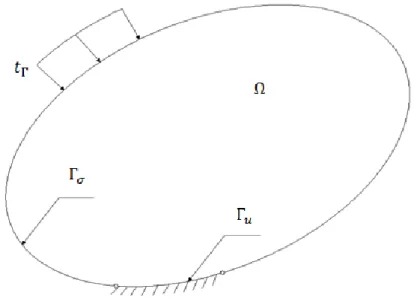
The general problem definition given above is particularized next for the solid mechanics application presented in Figure 2-1.

(25)

5 Under static conditions, the following equations govern the response of the domain to the external force ,

 equilibrium equation (2.3)  compatibility equation (2.4)  constitutive law (2.5)

In the above equations, is the displacement field, vectors and collect the stress and strain components, is the material stiffness matrix, represents the body force field, and and are the divergence and gradient operators. Equations (2.3) to (2.5) can be merged into the Navier equation,

(2.6)

The Dirichlet and Neumann boundaries of the domain are defined as the parts of the external boundary where the displacements ( and the tractions ( are known,

, on (2.7)

, on (2.8)

2.2 Weak-form approach to the problem

One of the most general ways to derive the finite element formulation associated to a given problem is to use its form as a starting point (Zienkiewicz et al., 2005). The weak-form of equations (2.1) and (2.2) is obtained after enforcing weakly these equations, using some arbitrary functions collected in bases and ,

(2.9)

where represents the transpose of vector .

If expression (2.9) is valid for any possible choice of and , it is equivalent to the local satisfaction of the differential equations (2.1) and boundary conditions (2.2). It is important to stress that the integrals in (2.9) must be proper, which poses certain restrictions on

(26)

6 the test functions and and on the trial functions that are used to approximate the unknown field u.

The Equation (2.9) is integrated by parts, to yield, in general,

(2.10)

Operators to present in the weak-form (2.10) normally contain lower order derivatives than the operators from the initial equations (2.1) and (2.2). This renders the choice of the approximation functions more flexible, as lower order degree continuity is required, although a higher degree of continuity is now necessary for the test functions and .

The weak-form approach is applied to solid mechanics problems by enforcing weakly the domain and boundary equations (2.6) and (2.8),

(2.11)

The kinematic boundary condition (2.7), defined on boundary , is not enforced because it is assumed to be respected a priori by the displacement field u. This so called “conformity constraint” must therefore be observed by the trial functions used to approximate the displacement field. The kinematic boundary is labeled essential boundary, as opposed to the natural boundary , on which boundary condition (2.8) is explicitly included in the weak-form.

Integrating equation (2.11) by parts, results:

(2.12)

As the choice of and is arbitrary, important simplifications can be achieved by setting at this point, to yield,

(2.13)

At the same time, choosing basis such to have on , makes the Dirichlet integral in (2.13) disappear and expression (2.13) simplifies to,

(27)

7 The FEM is based on the partition of the domain into smaller regions, called finite elements. In each of the finite elements, equation (2.14) remains valid. Using this approach, the integral equation (2.14) can be reduced to a set of algebraic equations by approximating the displacement field in the domain of an element as,

(2.15)

In expression (2.15), matrix collects a subset of a function basis and the unknown vector lists their weights.

According to the Galerkin principle, the test functions are also expanded in the same basis,

(2.16)

Inserting expressions (2.15) and (2.16) into the weak-form (2.14), yields,

which is equivalent to,

(2.17)

(2.18)

where

(2.19)

(2.20)

System (2.18) is symmetric and, when written for the whole finite element mesh, block-diagonal. After its solution, the finite element approximations of the displacement, strain and stress fields are recovered using definition (2.15) and equations (2.4) and (2.5), respectively.

2.3 The virtual work principle as a weak-form

For the structural engineer, it is often more appealing to reach the finite element formulation from the physically-meaningful virtual work principle.

In order to formulate the virtual work principle, it is necessary to enunciate the basic concepts related to internal and complementary energies, and potential and complementary potential energies.

(28)

8 Considering a deformable body subjected to a uniaxial state of stress, and hence experiencing a longitudinal deformation, infinitesimal changes in stress cause infinitesimal increases in deformation . The infinitesimal variation of the internal energy density is defined as the work of the stresses on the deformation :

(2.21)

or, admitting geometrical linearity,

(2.22)

It is now possible to define the internal energy density (associated to the uniaxial stress state) as the sum of all infinitesimal variations between zero and the final strain ( ),

(2.23)

Considering the same body, under the same conditions, the infinitesimal variation of the complementary energy density is defined as the variation of the stress on the total deformation of the body:

(2.24)

Figure 2-3 - Internal energy density and its variation

Figure 2-2 - Complementary energy density and its variation

(29)

9 and for infinitesimal deformations,

(2.25)

Thus, the complementary energy density associated to the uniaxial state of stress is defined as the sum of all infinitesimal variations between zero and the final stress ( ),

(2.26)

It is important to define a correlation between the internal energy density and the complementary energy density, as their sum is equal to the work of a constant stress field on the total strain,

(2.27)

The potential energy of a mechanical system is the difference between the total internal energy of the system ( and the work of the applied external and volume forces ( ),

(2.28) where, (2.29)

in which is the initial state of deformation.

The complementary potential energy of a mechanical system is defined as the difference between the total complementary internal energy of the system and the work of the

reactions on the enforced boundary displacements ( ,

(2.30) where, (2.31)

(30)

10 The virtual work principle states that, on a deformable body in equilibrium, the exterior work is equal to the internal work, i.e. the work of the applied forces and reactions on the displacement field is equal to the work of the stresses on the corresponding strains,

(2.32)

By the application of the definitions (2.28) to (2.31) and the property (2.27), it is possible to reach the virtual work principle in the form of potential energies,

(2.33)

There is an immediate correspondence between the weak-form approach to the problem described in Section 2.2 and the virtual work principle. In fact, to create a weak-form it is sufficient to define a weighting function vector,

(2.34)

where represents any compatible virtual displacement field and its corresponding weights.

The choice of the test functions above allows the transformation of expression (2.32) into a weak-form equivalent statement,

(2.35)

As the virtual work principle must hold for any generalized displacements , expression (2.35) simplifies to the finite element system (2.18).

It should be noted that both weak-form and virtual work formulations can be used for linear and non-linear problems. However, the virtual work principle is restricted, in the presented form, to solid mechanics application.

2.4 Variational principle form of the problem

A more general, yet physics-based, approach to the FEM is provided by the so-called variational principles.

In order to approach the concept of variational principle, it is first necessary to define a functional scalar quantity,

(31)

11 (2.36)

where u is the unknown function and F and E are differential operators. A variational principle states that the correct solution of the problem is the one that makes stationary for arbitrary changes ,

(2.37)

Although variational principles do not exist for all well posed problems defined by valid partial differential equations, when they do exist, they offer some advantageous properties:

- form (2.37) is very well suited to the framework of the FEM; - the stiffness matrix always results symmetric/Hermitian.

Symmetric/Hermitian stiffness matrices may, at times, arise from weak formulations as well. When this happens, there exists a variational principle associated to the respective problem, although it may yet be unknown.

The existence and establishment of natural variational principles can be approached by considering the case of a physical problem defined by the partial differential equation

(2.38)

in which is a differential operator. It can be shown that natural variational principles exist if this operator is self-adjoint, that is,

(2.39)

for any two function sets and , where notation is used to designate boundary terms. If the requirement above is fulfilled, it is possible to write the function , from which the variational principle is obtained, as,

(2.40)

(2.41)

(2.42)

(32)

12 The application to solid mechanics is made by identifying forms (2.6) and (2.38), from which results,

(2.43)

The first step to obtain the variational principle is to determine if the operator is self-adjoint: (2.44)

which means that operator is indeed self-adjoint.

Once proven the self-adjointness of the operator , the existence of a natural variational principle is verified. This principle is given by the minimum potential energy theorem,

(2.45)

It is now possible to obtain the variational form of the solid mechanics problem by taking explicitly the differential of the potential energy ,

(2.46)

Analyzing and comparing forms (2.46) and (2.11), it is noted that the former represents a particular case of the latter. This fact is always true when variational principles exist. It is important to note that the use of variational principles is restricted to linear elasticity problems, due to the self-adjointness requirement for the operator .

(33)

13 The finite element formulation based on variational principles (known as the Rayleigh-Ritz method) is immediate when a variational principle exists. Using the approximation,

(2.47)

The differential variation of the functional is expressed as, (2.48)

In order to satisfy expression (2.48) for any arbitrary variation of , it is necessary that partial derivatives

to

are all null. As this system can immediately be written in the form

(2.18), it is adequate for direct application of the FEM.

For the solid mechanics problem, the finite element approximation of the potential function is,

(2.49)

where the first integral expression represents the stiffness matrix and the remaining expressions give the equivalent nodal forces, simplifying (2.49) to,

(2.50)

2.5 Error and convergence

The FEM is approximate in nature and the quality of its solution may result disappointingly low if its convergence properties are not well understood or appropriately handled. Consequently, the study of the quality of the solutions and of the means available to the analyst to improve it is an important issue in the FEM.

In essence, there are two methods capable of increasing the quality of the solutions obtained through the FEM:

 the h-refinement, that is based on the increase of the number of elements;

 the p-refinement, which consists of increasing the degree of the approximation functions.

(34)

14 The order of convergence ( ), when the leading dimension of the element is reduced h times is can be determined by,

_(2.51)

where p is the largest degree of a complete polynomial used for the construction of the basis of the finite element.

For instance, if the approximation functions are linear ( ) and the leading dimension of the element is reduced to half, it should be expected that the errors would decrease roughly four times.

In complex engineering structures, it is generally computationally ineffective to use the same level of h-refinement throughout all of the structure. The h-refinement should thus be localized, that is, confined to areas where sudden variations of the unknown fields are expectable. A typical example is the stress concentration zones, such as those occurring around wedges, notches, cracks and localized applied loads.

The mesh refinement strategy holds several advantages over the alternative p-refinement such as its easy implementation, the possibility of performing localized

refinements and the use of the same type of element in all of the mesh, which reduces the time spent on the element generation1. However, the convergence obtained by increasing the number of elements is typically lower than the convergence obtained by increasing the degree of the approximation functions.

In commercially available finite element software, the most broadly used method to increase the quality of a solution is the mesh refinement. Some software, however, also allow

the analyst to choose between a (typically limited) number of elements with different p-refinements.

In order to achieve the convergence of a certain solution, obtained through the FEM, to the exact solution, there are two convergence criteria that must be fulfilled. The first criterion states that the finite element basis must be chosen such as to be able to represent exactly a rigid body displacement of the element, if such displacement is physically possible. Thus, for an element with nodes,

(2.52)

1_{Although the use of elements with different p-refinements in the same mesh is not theoretically}

impossible, the computational effort required for creating “connecting” elements hinders, in practice, localized p-refinement

(35)

15 that is, the shape functions must form a partition of unity. The capacity of the element to recover rigid-body motion ensures that the FEM solution steadily converges to the exact solution as the element size is decreased and indeed recovers it exactly in the limit, when the element becomes a point (and thus the rigid-body displacement is its exact solution). The second criterion states that the displacement approximation functions must be chosen such that the deformations generated at the interface of two adjacent elements are finite.

In order to illustrate the relevance of the mesh refinement towards the achievement of satisfactory results, two numerical examples are presented next. The first example is an eigenmode analysis of a rectangular plate and the second example is a static analysis of a tension coupon with a circular hole in its center. In both examples, the analytic solution is available, which allows for a relevant analysis of the effect of the mesh refinement on the finite element solution. Both examples are implemented using the finite element software PATRAN and MSC.-NASTRAN.

a) Calculation of the eigenmodes of a rectangular plate

 Description of the problem

Consider the rectangular plate represented in Figure 2-4, constructed of aluminum and simply supported on all of its edges. The equation (2.53) providing the analytic solution of the first eigenfrequency was derived by Feldmann et al.(2009).

(2.53) where, _(2.54)

In the above equations, E is the Young’s modulus, is the Poisson ratio, stands for the thickness of the plate, is the material density and and are the larger and smaller dimensions of the plate, respectively.

(36)

16

Dimensions and Properties

L 1200 mm B 800 mm t 6.25 mm E 68900 MPa 0.33 27 kN/m3

Table 1 - Dimensions and properties of the rectangular plate Figure 2-4 - Rectangular plate

 Testing setup

The Feldmann problem is solved next, using the data listed Table 1.

Under these conditions, equation (2.53) yields a value of 33.868 Hz for the first eigenfrequency. To perform the finite element analysis, the plate is discretized using 4-node, 24 degrees-of-freedom (DOF) square shell elements available in MSC.-NASTRAN.

In order to assess the convergence to the analytic solution, the analysis is performed using elements with leading dimensions comprised between 2 and 40 cm.

(37)

17

 Finite element results

The deformed shapes corresponding to the first eigenmode and the respective eigenfrequencies are given in Table 2 for each of the analyzed situations.

Element dimension: cm Element dimension: cm

f = 29.29 Hz f = 32.546 Hz

Element dimension: 1 cm Element dimension: cm

f = 33.445 Hz f = 33.567 Hz

Element dimension: cm Element dimension: cm

f = 33.756 Hz f = 33.81 Hz

Table 2 - Deformed shape and eigenfrequency corresponding to the first eigenmode for different element dimensions

(38)

18 The effect of the mesh refinement procedure is clearly visible as the error decreases from 13.52% for the case of the coarsest mesh to 0.17% for the finest mesh. The price to be paid, however, is the computational effort, which increases exponentially with the total number of DOF, which ranges between 144 and 57600.

b) Static analysis of a tension coupon

 Description of the problem

Consider the tension coupon represented in Figure 2-5, constructed of aluminum, with a circular hole in its center and subjected to an edge load. The equation (2.55) providing the analytic solution of the maximum stress at the edge of the hole was derived by Pilkey & Pilkey (2008),

(2.55)

where is a stress concentration factor based on the net cross-sectional area, which can be

graphically determined from a diagram given in Pilkey & Pilkey (2008), and is the normal stress based on net area,

(2.56)

in which is the external load (applied as a distributed force on the respective boundary), is the thickness of the coupon, stands for the width of the element and for the diameter of the hole.

(39)

19

Dimensions and Properties

L 200 cm H 80 cm t 2,5 cm E 68.9 GPa 0,33 D 40 cm 10 kN

Table 3 - Dimensions and properties of the tension coupon

 Numerical setup

The theoretical solution of the maximum stress at the edge of the hole is obtained using the data listed in Table 3, and yields a value of 2170 kPa. The discretization of the plate is performed using square shell elements, the same type of elements as in the previous example.

To achieve the convergence to the analytic solution, the analysis is performed using points as mesh “seeds”. By optimizing the number and position of these points, as well as the finite elements length, more accurate results are obtained.

 Finite element results

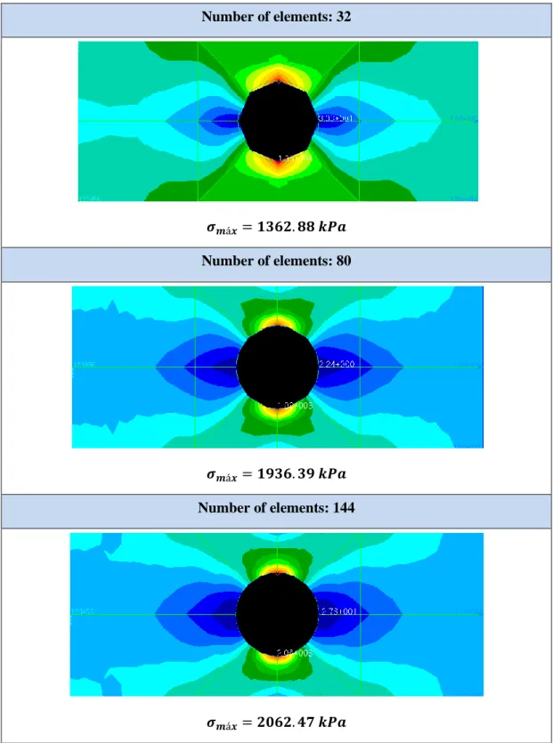
The stress diagrams and the values of the maximum stresses corresponding to the analyses performed with increasing number of elements are presented in Table 4. The orange areas of the stress diagrams represent the zones where the stress is larger, and the blue areas are the zone where the stresses are minor.

(40)

20 Number of elements: 32 Number of elements: 80 Number of elements: 144

Table 4 – von Mises stress diagram and maximum von Mises stress for increasing number of elements

(41)

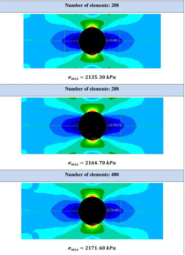
21 Number of elements: 208 Number of elements: 288 Number of elements: 480

Table 4(cont.) – von Mises stress diagram and maximum von Mises stress for increasing number of elements

(42)

22 The mesh refinement yields significant effects on the accuracy of the results, as the error decreases from 37.19% for the coarsest mesh, with 32 elements, to 0.074% for the finest mesh, with 480 elements. However, the number of DOF increases from 768 to 11520.

(43)

23

3. STRUCTURAL OPTIMIZATION

Many engineering problems involve structural optimization. Their goal is to satisfy certain requirements (e.g. limit state conditions) while minimizing certain quantities (e.g. resources spent) and maximizing others (e.g. structural safety). The requirements to satisfy are called restrictions and the functions to minimize/maximize are called objective functions. Optimization problems can be classified in three categories:

 Size optimization problems, which typically consist of the calibration of the cross sectional properties and dimensions of the structural elements. An example of a size optimization problem is the weight minimization of a truss structure by varying the cross-sectional areas of each element (Figure 3-1). The constraints are the allowable stress in all members and possibly, the displacements of selected nodes;

 Shape optimization problems, which consist of the optimization of the boundary shape, generally used to reduce stresses or to make the stress distribution uniform with no increase of structural weight. An example of such problem is the shape optimization of the Michell’s arch2 to achieve weight minimization by varying the coordinates of the nodes, with a displacement constraint at the loaded node;

2_{Structure named in honor of Anthony George Maldon Michell, an Australian mechanical}

engineer who played an important role in the development of structural optimization by publishing in 1904, his work “The limits of economy of material in frame structures”.

(44)

24

 Topology optimization problems, in which the goal is to determine the optimal distribution of material, given the design space, boundary conditions, loads and required design performance. An example of topology optimization problem is the optimization of a bicycle frame (Figure 3-3). The design process starts from the definition of a design area domain (the left-hand-side of Figure 3-3) and evolves towards the optimized material distribution (the right-hand-side of the same Figure), observing, at all times, a range of strength and displacement constraints.

Some key numerical methods to find extrema of functions (which constitute an essential part of all structural optimization procedures), are introduced in the next Section. The general description of the methods is followed by their application to two optimization problems from the engineering practice.

Figure 3-3 - Topology optimization problem: bicycle frame topology optimization Figure 3-2 - Shape optimization problem – Michell’s arch shape optimization

(45)

25

3.1 Introduction to the minimization

3

of functions

Given a function of variables, the main objective of a generic minimization problem is to find the values of all variables ( ), that correspond to a minimum of . Besides this primary objective, the minimization method should be computationally fast, consume limited resources and accommodate additional constraints applied on the function’s variables.

The minimization methods presented in this Section are aimed at identifying local, rather than global minima of functions. A global minimum is defined as the lowest value of the function on a search interval, while a local minimum stands for the lowest value of the function in a finite neighborhood, but not necessarily on the entire search interval. It is important to note that both minima may either correspond to a null gradient point or be on the interval’s boundary. Clearly, finding the global minimum generally yields better practical results than local minimum. However, as many methods of finding the global minimum are simply based on comparing local minima, only the latter will be treated here.

Relative to the constraints posed on the function’s variables, the minimization problem may be unconstrained or constrained. The unconstrained minimization is used when no constraints are applied on the variables, while the constrained minimization occurs when restrictions are enforced on the variables. Within the constrained type of minimization, there are three different types to be considered:

- Simple: the restrictions are simply used to limit a search interval;

- Linear programming: the constraints are linear functions of the same variables;

- Higher degree programming: the constraints are higher degree functions of the same variables.

Except for some particularly simple cases, determining analytically extrema of functions is not a straightforward task, so numerical methods are typically used instead. A classification of some of the most common methods for functions minimization is given next. For functions of a single variable (1D minimization), the methods can be classified as:

- Methods that do not require computation of derivatives:

 The Golden Search method

 The Brent method

- Method that do require the computation of derivatives:

 The Brent method, modified

3_{It should be noted that the extremum-finding methods described in this section are invariant to}

whether the extremum is a minimum or a maximum. For simplicity and without lack of generality, minimum extrema are adopted in this presentation.

(46)

26 For functions of N variables, the methods presented here are:

- Methods that do not require computation of gradients:

 The Downhill Simplex method

 The Powell method

- Methods that do require computation of gradients:

 Conjugate gradient methods (Fletcher-Reeves, Polak-Ribiere)

 Quasi-Newton methods (Davidon-Fletcher-Powell, Broyden-Fletcher-Goldfarb-Shanno)

All these methods are briefly described in the next sections.

3.2 One-dimensional minimization (unconstrained)

3.2.1 Golden search method

This method is one of the simplest minimum-finding methods, although not very fast in convergence. Employed to search for the minimum value of a continuous function, the method starts with the calculation of 3 abscissas (the bracketing points such that,

After this, a new sampling point ( is chosen between and the furthest away limit of the bracketing interval ( ). Then, based on the value of the function in the bracketing points, one of them is discarded by the following procedure:

- If (Figure 3-4) - Else

(Figure 3-5)

These criteria ensure that the minimum is, at all times, inside the bracketing interval. The point-discarding process described above repeats itself and allows for a gradual narrowing of the searching interval, until it becomes smaller than a tolerance, never inferior to , being the machine precision.

(47)

27 Although slow, in general, the convergence of the method can be improved by taking the new sampling point (d) such that the length between b and d is given by , being the golden ratio4 0.38197, and the distance between b and the furthest away point of the bracketing interval.

4_{This number, along with 0,61803, are well-known for their importance in the old Greek}

architecture. Buildings with the dimensions related through these constants were considered aesthetically pleasing.

Figure 3-4 - Bracketing interval when f(d)>f(b)

(48)

28

3.2.2 Brent’s method in 1D

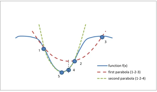
This method is the most effective when the objective function´s behavior near its minimum is smooth and hence is possible to use a parabola to approximate the function. Just as in the Golden Search method, the starting point of the Brent’s method involves the definition of three (bracketing) points. However, unlike the Golden Search method, the bracketing points are used to create an interpolating parabola. It is possible to prove that the extremum of this parabola is located at:

(3.1)

The process is illustrated in Figure 3-6. In the first iteration, the parabola passes through the first three bracketing points 1-2-3, and has an extremum at point 4. The second iteration uses the new bracketing interval obtained from the first interval by discarding the abscissa corresponding to the largest function value. In the case presented in Figure 3-6, the new parabola will thus pass through points 1, 2 and 4.

Although this method provides quadratic convergence, it has certain disadvantages when compared to the golden ratio method, such as the possibility of having iterations that yield maxima instead of minima, or the numerical problems encountered when approaching the

Figure 3-6 - Approximation of a function's minimum according to Brent's method function f(x) first parabola (1-2-3) second parabola (1-2-4) 1 2 3 4 5

(49)

29 extremum. This last issue is caused by the instability of equation (3.1), as the method gets closer to the extremum, due to the decreasing distance between the interpolation points.

3.2.3 Brent’s method, with first derivates

When information about the function’s first derivative is available, it must be handled with care. Indeed, the two most obvious strategies may be problematic at a deeper consideration:

- The elaboration of a numerical root-finding algorithm to find the root of the function’s derivative, using only derivative information, has problems related to the issue of distinguishing between a maximum and a minimum and to the fact that the derivative in an outer point of the bracketing interval points to the exterior of this interval.

- The construction of a higher-degree polynomial approximation of the function, using the information on the function and derivative’s values, although sometimes adequate, may amplify the numerical errors when the bracketing interval decreases.

Instead of using the ideas presented above, the modified Brent’s method evaluates the derivative of the function in the middle of the bracketing interval in order to establish if the next bracketing point should lay on the left or the right side of the interval. Then, as shown in Figure 3-7, this derivative and the derivative of the second-best bracketing point so far (a) are interpolated to zero and the new point ( ) that results from this interpolation is included in the new bracketing interval. However, if the new point is not consistent with the side of the interval it should lay into (between points and ), the new point is dropped and substituted by point , chosen in the middle of the “correct” region, as shown in Figure 3-8.

(50)

30

Figure 3-7 - Linear interpolation yields a new bracketing point (d) in the acceptable region of the bracketing interval

Figure 3-8 - Linear interpolation yields a new bracketing point (d) in the unacceptable region of the bracketing interval

(51)

31

3.3 Multi-dimensional minimization (unconstrained)

3.3.1 Downhill simplex method

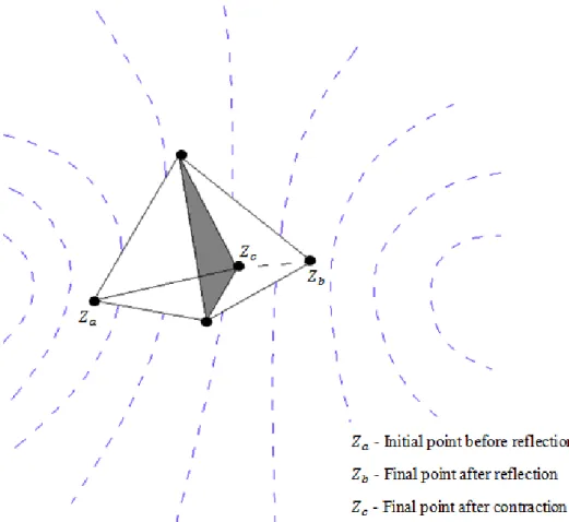
This minimization method uses a simplex, defined as a geometrical figure with N+1 points and all of their interconnecting lines and surfaces, where N is the dimension of the space the function is defined on. The simplex is constructed by taking one initial arbitrary point ( ) and one arbitrary side length ( ), from which it is possible to generate the remaining simplex points as,

(3.2)

where stands for the versor of each one of the N directions in the function’s space.

The downhill simplex method uses the simplex to evaluate the objective function at each node of the figure, in order to identify the node that corresponds to the highest value of the function. Once this point is found, a new trial point is obtained as the “symmetric” of the largest-valued point on the other side of the simplex. This procedure is called “reflection” and is illustrated in Figure 3-9. After the reflection, a new function evaluation takes place at the new point and if the new value is lower than the previous highest one, the previous point is discarded and a new simplex is constructed using the new point. Conversely, if the new point corresponds to a value larger than the largest of the previous simplex, the new point is discarded and a new trial point is defined on the same vertex, but closer to the center of the simplex. This procedure is called “contraction”. (Press et al., 1992)

(52)

32 Although this method does not require the use of derivatives, many evaluations may be needed at every iteration for the simplex to approach the minimum. On the other hand, the method is remarkably robust and particularly efficient for functions with unstable behavior.

It is important to note that this method is the only N-dimension minimization technique that does not use 1-dimension minimization as its basis.

3.3.2 Powell’s method

Powell’s method is a numerical technique for unconstrained minimization that does not require the calculation of derivatives and consists of sequences of 1-dimension minimizations.

The method uses a sequential minimization of the function, which takes place in different directions:

- The function is minimized in an arbitrary direction (x);

Figure 3-9 - "Reflection" and “contraction” of the highest value point from the initial simplex in a valley simulated by the blue dashed lines

(53)

33 - Taking the minimum found in the x direction as a new starting point, the function is

now minimized in another direction (y);

- This process repeats itself until the function’s minimum is found.

Obviously, this method requires the availability of a line-minimization algorithm, to take as input an arbitrary initial position vector P and the minimization direction versor , and to output the function’s minimum in the direction,

(3.3)

Depending on the adopted line minimization technique, the method may reach quadratic convergence (Chapra & Canale, 2006). The fact that it does not necessarily require the evaluation of function’s derivatives is also an advantage. However, the method may require a very large number of iterations to converge when the minimization directions correspond to the directions of the referential and the function is characterized by a long narrow valley, not aligned to any of the axes. The reason for this is that the minimization of the function in one direction generally compromises anterior minimizations in orthogonal directions, leading to the necessity of restoring the minima in the anterior directions and the process repeats itself.

To avoid this issue, it is desirable to identify some directions that do not interfere with each other, so that the minimization along one is not hindered by the minimization along the other. These are called “conjugate directions” and their theory is briefly reviewed in the next Section.

3.3.3 Conjugate directions

Consider the expansion in Taylor series of a function , around a point ,

(3.4)

which can be written in the equivalent matrix form:

(3.5)

where

(3.6)

(3.7)

(54)

34 Consider next the Taylor series expansion of the gradient of the function . The derivative of the function in a generic direction is,

(3.8)

and applying the same procedure for all directions i,

(3.9)

Using expression (3.6), result (3.9) is put in the form,

(3.10)

From result (3.10), it follows that the change of the gradient when one successively moves from point in directions and (not necessarily orthogonal) is,

(3.11)

The necessary and sufficient condition for this change not to be affected by a subsequent minimization in direction is for the vector to be orthogonal to the anterior change of gradient,

(3.12)

When the condition (3.12) is satisfied for two direction vectors, they are labeled conjugate directions. When this condition is satisfied for a whole vector set, a conjugate set is obtained.

The minimization along a set of conjugate directions lifts the necessity of performing various passages through each direction, requiring only one passage through all directions, if the analyzed function is a quadratic form, that is, if the expression (3.5) is exact. If the Taylor expansion is not exact, more iterations will be needed, but the convergence is still generally much faster than that of the Powell’s method.

The efficient construction of conjugate directions is important as it may be the most computationally demanding process in the conjugate gradient methods. To obtain conjugate directions it is necessary to consider, first, an arbitrary initial vector, , and to create a set of vectors, , such that the expression (3.12) is verified for any pair of these vectors,

, for any (3.13)

Application of definition (3.13) for computing the conjugate directions involves the computation of the Hessian matrix, which is generally difficult to accomplish. Therefore, it is

(55)

35 important to recover the conjugate directions without knowledge of the Hessian matrix. This is only practically achievable in an exact manner for quadratic functions. However, the method used to do so produces good approximations of the conjugate directions even when the function is relatively far from quadratic. Starting with a direction vector and an auxiliary vector

, the method successively constructs the recursive sequence,

(3.14) where, (3.15)

It can be shown that vectors and satisfy the following orthogonality conditions:

(3.16)

Consequently, if the Hessian matrix was known, it would be possible, by the application of (3.14) and (3.15), to construct the sequence of conjugate directions . However, as the Hessian matrix is not known, an alternative approach must be identified. Consider now that the auxiliary vectors are defined as the gradient of the function in the current point ,

(3.17)

Now, by the application of the equation (3.10), the function’s gradient computed in a point located at a distance along a direction is,

(3.18)

Setting as the distance between the initial considered point and the minimum in direction , and defining

(3.19)

equation (3.18) is identical to the second equation of system (3.14). Through this method, it is therefore possible to construct the sequence of vectors without any knowledge on the Hessian matrix.

Concluding, considering an arbitrary initial point , the procedure to obtain the conjugate directions is based on the following steps: