Macroprudential and Monetary Policies:
a Dynamic Stochastic General
Equilibrium Model-Based Perspective
Pesce, Simone
152216027
Thesis written under the supervision of Professor Gomes, Sandra
Dissertation submitted in partial fulfilment of requirements for the MSc in
Economics with major in Macroeconomic Policy, at Universidade Católica
Portuguesa and for the MSc in Economics and Finance, at University of
Naples Federico II, September 2018.
Macroprudential and Monetary Policies: a Dynamic Stochastic General Equilibrium Model-Based Perspective
By SIMONE PESCE1
Católica-Lisbon School of Business and Economics
Abstract
The increased emphasis on macroprudential policies since the global financial crisis has led to an increasingly rich literature on this subject. In this thesis, I use a DSGE model with borrowing constrained agents to study the impact of loan-to-value countercyclical macroprudential policies. By modelling a LTV ratio as a Taylor-type rule, I perform several simulations with different shocks in order to assess the macroeconomic impact, the transmission mechanism and possible (conflicting or complementary) interaction with monetary policy. I address the importance of policy design characteristics such as degree of reactiveness and graduality in the policy response from the macroprudential authority. The results show that the LTV ratio, by reacting to house prices growth, reduces the credit contraction associated with shocks arising in the housing sector. The sensitivity analysis suggests for the implementation of a smooth reaction of the policy to changes in house prices, which appears to better contain the fluctuations in credit. Regarding the interaction with monetary policy, simulations show that monetary and macroprudential policies are complementary when fluctuations are demand-base (i.e. housing preference shock) but they are conflicting when the shock is from the supply-side (i.e. housing productivity shock). Last, sensitivity analysis is performed with regard to the macroeconomic variable that the LTV ratio responds to.
Resumo
A maior ênfase dada à política macroprudencial desde a crise financeira global levou a uma crescente literatura sobre este assunto. Nesta tese, eu uso um modelo estocástico de equilíbrio geral com agentes com restrições ao endividamento para estudar o impacto de políticas macroprudenciais contracíclicas com base no rácio entre o empréstimo e o valor do imóvel que serve como colateral (loan-to-value, LTV). Ao modelizar o rácio LTV como uma regra do tipo Taylor, eu faço várias simulações com diferentes choques para avaliar o impacto macroeconómico, o mecanismo de transmissão e possíveis interações com a política monetária (quer complementares quer em sentidos contraditórios). Eu analiso a importância das características do desenho da política tais como a intensidade de resposta e o gradualismo na resposta de política da autoridade macroprudencial. Os resultados mostram que o rácio LTV, ao reagir ao crescimento dos preços de habitações, atenua a contração do crédito associada a choques com origem no setor de habitação. A análise de sensibilidade sugere uma reação gradual da política a variações dos preços de habitações, que parece conter melhor flutuações do crédito. Em relação à interação com a política monetária, as simulações mostram que as políticas macroprudencial e monetária são complementares quando as flutuações têm origem em choques do lado da procura de habitações mas existe conflito quando o choque é do lado da oferta de habitações. Em último lugar, é feita uma análise de sensibilidade com respeito à variável macroeconómica a que o rácio LTV responde.
Keywords: macroprudential policy, monetary policy, DSGE models, LTV ratio.
1 Email address: [email protected]
I would like to thank my supervisor, Professor Sandra Gomes of the Católica-Lisbon School of Business and Economics for the precious and constant support during the writing of this thesis. Her guidance throughout the process has been essential. I would also like to thank Professor Tullio Jappelli of the University of Naples Federico II for his suggestions and readiness to help. Finally, I want to thank my family for the endless encouragement and my friends, who made this journey so special.
TABLE OF CONTENTS
1 Introduction ... 1
2 Literature Review ... 4
2.1 Macroprudential policies overview ... 4
2.2 Effects of the macroprudential policies ... 5
2.2.1 Loan-to-value ratio as a prudential tool ... 6
2.3 Macroprudential policies within DSGE models ... 8
2.4 Monetary policy interaction with macroprudential policies ... 11
3 The Model ... 16
3.1 DSGE Models ... 16
3.2 Model setup ... 16
3.2.1 Households ... 17
3.2.2 Firms and technology ... 19
3.2.3 Monetary and Macroprudential Policies ... 21
3.2.4 Equilibrium ... 22
3.4 Calibration ... 22
4 Impulse Responses Analysis ... 24
4.1 Implementation in Dynare ... 24
4.2 Housing Preference Shock ... 25
4.3 Housing Productivity Shock ... 31
4.4 Monetary Policy Shock ... 38
4.5 Sensitivity Analysis ... 43
4.5.1 Credit Growth and other settings ... 43
4.5.2 LATW ... 47
5 Concluding Remarks... 50
Appendix ... 52
LIST OF FIGURES
Figure 1: Housing Preference Shock - Original vs Benchmark ... 26 Figure 2: Housing Preference Shock – Original vs Benchmark – House Prices and LTV Ratio ... 27 Figure 3: Housing Preference Shock - Benchmark vs ∅qM= 0.5 and ∅qM= 20 ... 28 Figure 4: Housing Preference Shock - Benchmark vs ∅qM= 0.5 and ∅qM= 20 – House Prices and LTV Ratio ... 29 Figure 5: Housing Preference Shock - Benchmark vs ρM= 0 and ρM= 0.95 ... 30 Figure 6: Housing Preference Shock - Benchmark vs ρM= 0 and ρM= 0.95 – House Prices and LTV Ratio ... 31 Figure 7: Housing Productivity Shock - Original vs Benchmark ... 33 Figure 8: Housing Productivity Shock - Original vs Benchmark - House Prices and LTV Ratio ... 33 Figure 9: Housing Productivity Shock - Benchmark vs ∅qM = 0.5 and ∅
q
M = 20 ... 35 Figure 10: Housing Productivity Shock - Benchmark vs ∅qM = 0.5 and ∅
q
M = 20 – House Prices and LTV Ratio ... 35 Figure 11: Housing Productivity Shock - Benchmark vs ρM= 0 and ρM= 0.95 ... 37 Figure 12: Housing Productivity Shock - Benchmark vs ρM= 0 and ρM= 0.95 – House Prices and LTV Ratio ... 37 Figure 13: Monetary Policy Shock - Original vs Benchmark ... 39 Figure 14: Monetary Policy Shock - Original vs Benchmark – House Prices and LTV Ratio ... 39 Figure 15: Monetary Policy Shock - Benchmark vs ∅qM = 0.5 and ∅qM = 20 ... 40 Figure 16: Monetary Policy Shock - Benchmark vs ∅qM = 0.5 and ∅
q
M = 20 – House Prices and LTV Ratio ... 41 Figure 17: Monetary Policy Shock - Benchmark vs ρM= 0 and ρM= 0.95 ... 42 Figure 18: Monetary Policy Shock – Benchmark vs ρM= 0 and ρM= 0.95 – House Prices and LTV Ratio ... 42 Figure 19: Housing Preference Shock - Benchmark vs Credit Growth ... 44 Figure 20: Housing Preference Shock - Benchmark vs Credit Growth – House Prices and LTV Ratio ... 44 Figure 21: Housing Productivity Shock - Benchmark vs Credit Growth ... 46
Figure 22: Housing Productivity Shock - Benchmark vs Credit Growth – House Prices and LTV Ratio ... 46 Figure 23: Housing Preference Shock - Benchmark vs Augmented TR ... 48 Figure 24: Housing Preference Shock - Benchmark vs Augmented TR – House Prices and LTV Ratio ... 48 Figure 25: Housing Productivity Shock - Benchmark vs Augmented TR ... 49 Figure 26: Housing Productivity Shock - Benchmark vs Augmented TR – House Prices and LTV Ratio ... 49
1 Introduction
Macroeconomic policies involve a large set of targets (e.g. economic and financial stability, price stability) and instruments (e.g. interest rates, and fiscal tools). To inform policy decisions, economists use a large set of tools to analyse the impact of different policies, including theoretical models and empirical analysis.
Following the 2007-09 crisis, these instruments have been under discussion both in the academia and in policy institutions and it has become clear that to guarantee the safety of the economic and financial system there is the need to encompass a broader set of goals compared to the pre-crisis regulation. Even though several factors lead to the financial crisis, there is some agreement that inadequate or insufficient prudential policy did play a role in the building up of the crisis. Indeed, there was the need to go beyond a purely micro-based approach to financial regulation and supervision thus leading to the introduction of macroprudential perspective in the framework. So, one can say that nowadays macroprudential policy is seen as the policy aiming at achieving financial stability and containing systemic risk2 (Galati and Moessner (2013)).
A successful implementation of macroprudential policies has to take into account that they interact with other types of policies, in particular with monetary policy. In theory, if monetary and macroprudential policies have different objectives they should use separate sets of instruments (Tinbergen principle). In fact, monetary policy primary objective is generally accepted as price stability, whereas for macroprudential policy it is financial stability. Even though these goals are necessarily complementary to the well-functioning of an economy, in practice, however, the implementation of these policies may in certain circumstances be complementary, but in others conflicting behaviour may imply trade-offs. Recent research papers address this issue,3 inparticular through the use of Dynamic Stochastic General Equilibrium (DSGE) models that offer a theoretically consistent tool to address policy questions and which have become the workhorse macroeconomic
2 Systemic risk is the risk of collapse of an entire financial system (or banking sector), as opposed to
the risk associated with an individual institution (e.g. bank) that can be contained without harming the entire system. Systemic risk often arises within the activities of main financial institutions, often called “Too Big to Fail”. Given their importance for the functioning of the system (either due to size or interconnectedness) the risk exists that issues at the company level could trigger serious instability or collapse of the entire financial system. The rationale of macroprudential policies is to mitigate the risk and reduce the externalities affecting financial – and economic – stability.
models in policy’s evaluation over the last decades. Developments in DSGE models have been central in the macroeconomic literature over the last three decades. The initial Real Business Cycle (RBC) models by Kydland and Prescott (1982) and Long and Plosser (1983) among others focused on fluctuations in aggregate economic activity as an efficient response to exogenous technological shocks. These general equilibrium models are built upon solid microeconomic foundations (emphasizing agents optimizing behaviour and intertemporal choices). However, they had difficulty in accounting for some key properties of aggregate data and gave no room for monetary policy. Subsequently, modifications were introduced, e.g. nominal and real rigidities, giving rise to the so-called New Keynesian models. Such features allow these models to explain many characteristics of modern economies and to overcome some of the previous model’s shortcomings. These New Keynesian DSGE models are set up on the seminal work of Smets and Wouters (2003-07) and Christiano, Eichenbaum and Evans (2005) and have become broadly used not only in the academia but also in policy institutions.4 When taken to the data discipline through estimation, they have been shown to fit aggregate data reasonably well and also to do well in forecasting (see for example Smets and Wouters, 2003). Furthermore, a greater emphasis has been given to the financial sector when analysing economic issues with these models, especially since the Global Financial Crisis (GFC).
The study of macroprudential policies has gained relevance in the macroeconomic literature but this literature is far from reaching a consensus on its objectives and, especially, preferred instruments. This increased interest in the literature led to many research papers that introduced macroprudential tools (e.g. loan-to-value (LTV) ratios, limits on credit growth and other balance sheets restrictions, countercyclical capital and reserve requirements) in DSGE models to evaluate their implementation and effectiveness.5
The focus of this thesis fits in within this literature, by focusing on the impact of macroprudential policy on macroeconomic outcomes, how it impacts the transmission mechanism of shocks and how it interacts with monetary policy. The focus is on
4For example, the Federal Reserve System, the European Commission, the International Monetary
Fund, the Bank of Israel, the Czech National Bank, the Sveriges Riksbank, the Bank of Canada, and the Swiss National Bank use such models.
systematic policies, i.e. adjustments in policy as a response to changes in macroeconomic variables. In particular I focus on borrower-based polices, where the policy instrument is the LTV ratio. The analysis is based on a New-Keynesian DSGE model with a housing sector and collateral constraints, originally developed by Iacoviello and Neri (2010). The macroprudential policy is modelled in a Taylor-type rule to respond to macroeconomic variables (i.e. house prices growth). Since the original model does not include this policy feature, the introduction of the macroprudential rule could affect the agents’ behaviour. However, by using a microfounded model where parameters are structural, I assume that the calibrated parameters of the model are invariant to this policy change. However, if the model is not fully correctly specified (as discussed by Cogley and Yagihashi (2010)), this may not be the case and the analysis could be subject to the Lucas critique.6
The thesis is structured as follows. Section 2 presents a review of the literature on macroprudential policies and the use of DSGE models to assess its impact as well as its interaction with monetary policy. Section 3 presents the DSGE model used in the analysis and the calibration of the main parameters. Section 4 describes the simulations conducted in the model. Section 5 presents the conclusion, policy and institutional remarks and highlights potential future research questions.
6 Structural parameters should not change with economic policies. If a microfounded model is not
2 Literature Review
2.1 Macroprudential policies overview
The 2007-09 financial crisis has made clear that there is the need go beyond a purely microeconomic approach to financial regulation and supervision. Even though macroprudential tools have been used for some decades, its widespread use is more recent. The introduction of a macroprudential view to regulation started with the September 2010 reform of the international regulatory framework. At that time, the Basel Committee for Banking Supervision (BCBS) proposed a number of reforms to reinforce not only micro-prudential regulation but also to introduce a macromicro-prudential focus to address system-wide risks, given the interaction between the business cycle and the financial system and institutions. It has represented a necessary response to the lack of instruments to help predict and face the build-up of financial imbalances, which usually turn out to have severe macroeconomic consequences.
Macroprudential policy’s main objective is generally financial stability, though this has not been given a clear and precise definition (like for price stability); also, the set of potential instruments is large and no standard taxonomy has been identified.
Regarding the risks that macroprudential policy aims to mitigate, these include:
excessive credit growth and asset price inflation in particular fuelled by credit expansion;
extreme leverage from financial institutions;
Against this background, macroprudential policy works on two dimensions: reducing the tendency of the banking system to amplify the business cycle, both the booms and the busts, and increasing the resilience of the financial system. Even though the distinction identifies – theoretically – the targets, in practise there is still uncertainty regarding the appropriate macroprudential instruments to deal with each dimension.
According to Lim et al. (2011) some of the most frequent tools are capital conservation buffers, countercyclical capital buffer, LTV and DTI ratios. Regarding the second dimension, efficient tools are still under debate. According to Beau et al. (2014), considering the complex interconnection of the companies within the system, possible
solutions could consist in the combination of capital overcharge, contingent capital and bail-in debt7 for significantly important financial institutions.
Galati and Moessner (2013) distinguish between macroprudential tools orientated on the time dimension (procyclicality of the financial system) and tools focused on the cross-sectional dimension (how risk is distributed within the financial system and by how much each institution contributes to systemic risk). With respect to the first dimension, effective instruments are countercyclical capital requirements, (forward-looking) provisioning schemes as well as LTV ratios. Regarding the cross-sectional dimension, one of the major source of risk is correlated to large share of short-term liabilities in banks’ balance sheets: in order to counteract these vulnerabilities, tools such as net stable funding ratio or liquidity coverage ratio are notable examples. Moreover, the authors suggest that policies’ development can benefit from the identification of externalities of financial instability, based on the two referred dimensions of the analysis.
The vast set of macroprudential instruments available for policymakers poses a challenge for the evaluation of the impact of the policies (section 2.2) as different tools are able to affect distinct exposures to instability. An adequate implementation likely combines several instruments. According to Claessens (2015), one of the most widely used tools is the LTV ratio so I assume this to be the macroprudential policy tool in the DSGE model used in the simulation analysis. For these reasons, section 2.2 is dedicated to review the evidence on the effects of implementing macroprudential policies but gives special focus to LTV-based policies. Section 2.3 presents recent applications of LTV ratio in the DSGE models framework. Section 2.4 focuses on the way macroprudential policies interact with monetary policy.
2.2 Effects of the macroprudential policies
A crucial issue faced by researchers and policymakers is the assessment of the impact of the macroprudential policies. The difficulty comes from the limited amount of data available, though experience with these policies is growing, and from different implementations across countries. The complexity is associated also with the
7 These are subordinated securities that are converted to common equity when certain conditions are
satisfied. The difference between contingent capital and bail in debt is that the latter is extended to senior debt securities of the financial institutions.
interrelationship with other types of policies, e.g. microprudential policies, and other macroeconomic policies that can support financial stability, such as monetary policy (see section 2.4) and fiscal policy.8
The impact of macroprudential policies has been analysed in the literature in recent years (for a recent survey see Galati and Moessner (2017)). Boar et al. (2017), using data for a panel of 64 advanced and emerging market economies,9 show positive effects of macroprudential policies’ implementationand find that countries are particularly active in using macroprudential policies have higher and less volatile per capita GDP growth. Interestingly, they find that these effects depend on the degree of country’s openness and financial development and that non-systematic macroprudential measures tend to be averse to growth.
Following the same strategy, Cerutti et al. (2017), using a dataset of 119 countries over the 2000-2013 period, show that emerging economies use policies more frequently and often related to the foreign exchange, while advanced economies concentrate more on borrowers’ constraints (such as LTV ratio). Furthermore, they find a negative link between the use of macroprudential policies and credit growth, even though they display heterogeneous impacts during the boom and the bust phases of the financial cycle, having less of an impact on busts.
Gambacorta and Murcia (2017) use granular credit registry data for several countries in South America and find that macroprudential policies have been successful in dampening credit cycles and reducing banking sector risk.
2.2.1 Loan-to-value ratio as a prudential tool
Given that there is no clear consensus on the use of different macroprudential instruments, the literature has analysed a wide range of possible tools. In this section, I focus on studies about LTV ratio policies in more detail as they are one of the most widely used prudential tool (Claessens (2015)) and it is the macroprudential tool I focus on in the empirical application. Imposing limits on the borrowing amount, in particular in mortgage loans, is a way to lower bank losses in case of default. The ratio is defined as the nominal amount of the mortgage loan divided by the value of the collateral.
8 On fiscal policy, see for example Borio (2009) and Blanchard et al. (2010).
9 The authors base their analysis on macroprudential data collected by Lim et al (2011, 2013), Kuttner
𝐿𝑜𝑎𝑛 𝑡𝑜 𝑉𝑎𝑙𝑢𝑒 𝑅𝑎𝑡𝑖𝑜 = 𝑀𝑜𝑟𝑡𝑔𝑎𝑔𝑒 𝐴𝑚𝑜𝑢𝑛𝑡
𝐴𝑝𝑝𝑟𝑎𝑖𝑠𝑒𝑑 𝑉𝑎𝑙𝑢𝑒 𝑜𝑓 𝑡ℎ𝑒 𝑃𝑟𝑜𝑝𝑒𝑟𝑡𝑦
Changes in the maximum LTV ratios will thus impact the behaviour of credit. Research has focused on measuring the impact of LTV caps across different countries. Quantifying these effects and identifying the channels through which the policy operates have represented large challenges for researchers. Focusing on the impact of the LTV policy on credit growth, one extensive study is a paper on Hong Kong, a country that has applied limits on loans since 1991. According to Wong et al. (2011), the LTV cap tightening in Hong-Kong controlled credit growth and the indebtedness of borrowers, which increase banks’ resilience to real estate price shocks. Additional information on the effects of LTV policy on the credit cycle is provided by Lim et al. (2011), Cerrutti et al. (2017) and Budnik and Kleibl (2018). These papers find a (negative) relationship between borrower-based measures and credit growth. Lim et al. (2011) also find that it is useful to combine more policies (e.g. LTV ratio addressing the wealth aspect and debt service-to-income (DSTI) for the income aspect) to ensure efficiency and limit the expansion of systemic risk. More focused on house prices and housing credit, Kuttner and Shim (2016) – using a panel of 57 countries from 1980 to 2010– show that changes in the LTV ratio were less successful in reducing (mortgage) credit growth compared to reduction in the DSTI ratio.10 Jácome and Mitra (2015),working with a small sample of countries, also find that reductions in LTV ratios (as well as DSTI ratios) were able to contain the growth of housing loans and improved performance of borrowers in repaying their loans, but their efficacy in reducing house prices growth is less evident.
Crowe et al. (2011) analyse tools to deal with real estate booms and point out three main policies: capital requirements, dynamic provisioning (it implies a higher loan loss provision for the bank during good times) and cyclical tightening/easing of the standards for real estate loans, e.g. LTV ratios. They find that the latter is the best mechanism (in terms of reduction of output gap’s volatility ) to hamper a real estate boom, in line with other empirical work,11 but it may suffer from a problem of policy design as there are
10 Kuttner and Shim (2016) provide as an example the offsetting of a reduction of the LTV ratio as
response to an increase in house prices that allows households to increase the amount that can be borrowed.
ways to circumvent the constraints imposed.12 In order to improve the efficiency of these policies, Crowe et al. (2011) call for a transparent communication from the authorities in charge, specifying that frequent and extreme changes to LTV ratios may lead to misleading signs and to policies that are driven by the real estate cycle. This points to a systematic behaviour of macroprudential policy authorities, including possibly some gradualism. This evidence partially motivates my choice of macroprudential rule used in the simulations (as discussed in Section 3).
Focusing on single country studies, recent analysis (Cassidy et al. (2016) for Ireland, Verbruggen et al. (2015) for the Netherlands) show that higher LTV ratios are related to higher probability of default of borrowers and losses for lenders. Compared to pre-crisis levels, these risks are lower partly due to the implementation of macroprudential policies, in particular reductions in the LTV ratio. Among other things, this includes less volatile house prices. With respect to the EU, during 2017 most of the policies introduced implied a tightening of borrowing conditions, caused by an increase in cyclical risks associated with the expansion phase of the business cycle.
In general, the crisis demonstrated the need and the importance of having a macro-view of regulation through the use of prudential policies. Even though some work has been done, more is required to assess and correctly establish the impact of such policies and, most important, to understand through which channels they impact the economy in order to inform the policymaker. Against this background, DSGE models are a useful laboratory to address these questions. My thesis fits in this branch of the literature by experimenting an LTV policy rule in a medium scale DSGE model. As such, next section presents a brief overview of this type of models while Section 2.4 focuses on the interaction between monetary and macroprudential policies.
2.3 Macroprudential policies within DSGE models
Macroprudential policies have been analysed recently in the context of DSGE models under different settings. Research on policies such as LTV ratio requires constraints to households to borrow against collateral (i.e. housing stock as in Iacoviello (2005) and Iacoviello and Neri (2010)). Results from DSGE models with borrower collateral
12There have been cases in which the LTV generated a peculiar real estate boom driven by
“short-cuts” to the constraints that it imposed. For example, limits to the amount on three-year loans in Korea generated a boom of loans with maturity of three years and one day.
constraint, such as Rubio and Carrasco-Gallego (2015), show that a LTV ratio rule helps to mitigate and control an expansionary phase of the business cycle by reducing credit growth, but it displays conflicting behaviour with monetary policy when the shock is arising from the supply side. Moreover, by designing a monetary policy rule that responds also to credit growth (i.e. it simulates a so-called “Lean against the Wind” (LATW) strategy, that involves a tighter monetary policy driven by financial stability purposes), it is optimal to have the central bank focusing on price stability and a macroprudential policy rule for financial stability.
Beau et al. (2014) analyse a DSGE model with borrow constrained entrepreneurs, and a macroprudential rule targets their credit growth. Their main result is that, in the presence of a financial shock, the macroprudential rule eases the response of monetary policy in counteracting the negative effects to the real economy. The dynamics of inflation is not greatly influenced by a LATW central bank, in addition to a macroprudential instrument, given the type of shocks that accounted the most for its fluctuation over their sample period. Lambertini et al. (2013) focus on a social welfare analysis within a DSGE model that includes heterogeneous agents (following Iacoviello and Neri (2010)). They show that an LTV ratio rule responding to credit growth is Pareto improving; furthermore, the optimized rules for monetary and macroprudential policies imply a lower volatility for house prices and credit, without performing an increase in inflation volatility. In contrast with the results showed in Beau et al. (2014), an interest rate rule that responds also to credit growth, in addition to an LTV ratio rule, is optimal in terms of social welfare.13 Studies with DSGE models with a banking sector focus on additional macroprudential policies, e.g. capital requirements. For example, Angelini et al. (2011) analyse a model for the euro area with credit frictions and countercyclical capital requirements as macroprudential tool. Monetary and macroprudential policies are modelled under two different settings: cooperation between the two institutions and independent conduct of policy. They find that when the economy is hit by supply shocks, the macroprudential rule produces low and negligible positive effects. Moreover, under the cooperative setting, this type of shocks generates excessive volatility in the policies’ instruments without stabilizing the macroeconomic variables of interest. On the contrary, under
13 Since the model exhibits two types of agents (savers and borrowers), when both LTV ratio rule and
interest rate respond to credit growth, a considerable share of the gains (in social welfare terms) goes to borrowers.
financial or housing shocks, the macroprudential rule produces considerable benefits in counteracting negative outcomes. Gains are higher when the institutions cooperate at the cost of high volatility in their respective policies’ tools.
Kannan et al. (2012) model the macroprudential rule to affect the bank lending rate (as a spread over the risk-free interest rate of the central bank) by imposing additional capital requirements to the banking sector. Their results are in line with the previous papers: having a macroprudential tool targeting credit growth allows to dampen negative effects arising from financial or housing sector shocks. At the same time, they find that it would be optimal to have no response from the macroprudential rule when the economy faces productivity shocks.
Other researchers have combined both capital requirements on the banking sector and households’ constraints in the DSGE framework. Carboni et al. (2013) analyse the interdependency of monetary and macroprudential policies for the euro area. The model includes financial frictions and a banking sector which is subject to capital requirements, firms and households are constrained on their collaterals. The main focus is on the impact on monetary policy when shocks arise from the macroprudential tools (counter-cyclical LTV ratio and capital buffer). In particular, an increase in capital requirements generates a contraction in the economy driven by higher margins applied by banks and a reduction in the provision of loans. In the case of a reduction in the LTV ratio, effects are more marked compared to capital requirements’ shock and eased by accommodative monetary policy.
In a similar setting, Brzoza-Brzezina et al. (2015) access the efficiency of macroprudential policies (i.e. LTV ratio and minimal capital adequacy) in a two-economy calibrated DSGE model of core and peripheral regions of the euro area. Given asymmetric shocks hitting the two regions both in the housing market and the banking sector, results show that the region - specific LTV ratio policy is more efficient in stabilizing output in the periphery than the capital requirements (common policy is not desirable from a welfare point of view). Moreover, a counter-cyclical macroprudential tool offsets partially the fact that monetary policy is common to both regions.
2.4 Monetary policy interaction with macroprudential policies
The following section focuses on the objectives, instruments and channels through which monetary and macroprudential policies operate and to which extent they are linked, leading to complementary or conflicting outcomes.
Central banks are in charge of the monetary policy in the country (or monetary union as in the case of Eurozone) in which they operate. Most central banks have a price stability goal.14 Regarding the instruments, a distinction need to be set up between “normal” times and crisis time (Svensson L. (2018)): the former usually consists of interest rate policy while the latter includes for example balance-sheet policies (large scale asset purchases also called quantitative easing) and lending at longer maturities.
Monetary policy aims at maintaining price stability and promoting economic growth whereas macroprudential policies aim at safeguarding the stability of the financial system. So, macroprudential policies interact with monetary policy actions and as such it can be argued that monetary policy has become more complex due to the more generalized used of macroprudential policy (Beyer et al. (2017)). In fact, even though these policies have different goals and use different instruments, the channels through which they operate are similar, so there is the need to understand how they interact with each other.
Beyer et al. (2017) classify the interaction between monetary and prudential policies in three major categories, based on the targets of the latter: asset, capital and liquidity-based. The interaction between these two policies goes both ways, e.g. monetary policy impacts prudential policies and vice versa. As explained by the authors, monetary policy affects prudential policies through:
Lending channel: the level of nominal interest rate set by the central bank influences capital requirements for banks and instruments designed for the credit demand side (e.g. LTV ratio). For example, under an accommodative monetary policy, the cost of funding is lower, thus it increases lending supply. The financial stability authority may need tighten capital requirements and the LTV ratio to increase financial institutions’ resilience to shocks. In particular, the dynamics could have a contractionary impact on the real economy since restrictions to credit
14 There are central banks (e.g. Federal Reserve in the U.S.) which have a dual mandate, embedding
demand and supply tend to vanish the positive effects coming from a loosening monetary policy.
Risk-taking channel: under an accommodative monetary policy banks are encouraged to take more risks (e.g. increasing the amount of risky assets in their portfolios and their leverage). As a response, the prudential authority may need to tighten capital requirements.
Prudential policies affect monetary policy through:
Lending channel: banks’ degree of leverage can influence the effects from (countercyclical) monetary policy, reducing further their credit supply. Indeed, highly leveraged financial institution will suffer more when an adverse shock hits the economy. Recent papers confirm a lower effectiveness of countercyclical monetary policy due to a tighter capital regulation. 15
Interest rate channel: prudential policies such as leverage ratios and risk-weighted assets measures tend to increase the cost of money in market’s transactions. This will be reflected in the interest rate markets which clearly is influenced by monetary policy. Other prudential measures as exposure limits tend to reduce funding opportunities for banks, which will be reflected in the money market rates;
Wealth channel: measures to contain credit demand (e.g. LTV ratios) influence and reduce the effects coming from a rise in asset prices, which imply a dampened impact from monetary policy through the wealth channel.
Borio and Zhu (2012) argue that the degree of impact of macroprudential constraints in the transmission of monetary policy is increasing, including direct and indirect effects: a change in the interest rate has direct effects on banks’ capital inflows (e.g. net interest margins, assets valuation and earnings) and indirect effects through impacts on non-banks’ balance sheets and on the overall macroeconomic conditions. Focusing on the risk-taking channel, Borio and Zhu (2012) argue that liquidity (to the extent at which agents can turn value into cash flows) is usually taken as exogenous16 - within the transmissions
15 Aghion and Kharroubi (2013), Budnik and Bochmann (2016), Maddaloni and Peydro (2013). 16 E.g. changes in collaterals’ values will impact borrowing capacity.
of macroprudential policy, while it is strongly influenced by risk perceptions and tolerance through monetary policy’s channels.
In addition to conventional monetary policy, non-standard monetary policy measures (such as the ECB’s Asset Purchase Program (APP)) interact with macroprudential policies. Antipa and Matheron (2014) perform several simulations with a DSGE model for the euro area of forward guidance policy which interact with a countercyclical macroprudential policy. They show that the countercyclical macroprudential policy (by relaxing the collateral constraint) increases the positive effects arising from forward guidance (in terms of inflation increase, compared to the case where the macroprudential policy is absent), even though their nature appears – theoretically – conflictive in the recovery phase: the latter aims at stimulating credit, the former to restrict it. On the same setting, Burlon et al. (2016) analyse17 the interconnection of local LTV ratios set by region-specific macroprudential authorities and the union-wide unconventional monetary policy (e.g. APP) in a euro area DSGE model where households have overly positive expectations about house prices growth. Results show that the local policies help in stabilizing the excessive borrowing as response to the accommodative monetary policy jointly with the APP. This analysis suggests interesting features of coordination between the ECB (at the monetary union level) and the regional macroprudential authorities. Coordination and interaction between the policies are issues arising from a natural conduct of these policies to pursue their objectives, breaking down the Mundell’s principle (Mundell (1962)) according to which “policies should be paired with the objectives on
which they have the most influence”: since the strategies affect the same variables, a call
for coordination may be necessary. In order to avoid situations in which macroprudential and monetary policies are working in a conflicting way (given that the former affects macroeconomic performance and that the latter may affect risk-taking incentives), a question of design and implementation of these policies arises.
Svensson L. (2018) argues that monetary policy cannot have financial stability as goal, since it is not able to achieve it: price stability does not ensure financial stability and monetary policy, in general, has no way to affect systematically and achieve sufficient resilience of the financial system. In support of this, the author looks at LATW policy
17 In the model, households have overly positive expectations about house prices growth, which they
applied by the Norges Bank and by the Riksbank. Svensson (2018) concludes that the costs are greater than the benefits of having monetary policy targeting also financial stability because “raising the policy rate simply has too small and uncertain effects on the
probability or magnitude of a financial crisis to match the certain substantial costs, in terms of lower inflation and higher unemployment” - Svensson L. (2018, pp.8).
Should there be coordination between monetary and macroprudential policies (even if the central bank is in charge for both)? Bean (2014) and Svensson (2018) support the idea that each policy should be conducted separately (during crisis prevention times), focusing on its goal and taking into account the conduct and the effects of the other policy, in order to achieve the best outcome. Separate conduct involves separate decision-making bodies, with separate goals and instruments. Under crisis management, full cooperation and coordination may be required, including all the relevant authorities.
In any case, the conduct of both policies will have to consider the effects they have on each other’s main objectives. Some authors argue that policy coordination may improve macroeconomic outcomes but concentrating more than one objective in one institution can imply credibility and accountability issues (IMF (2013), Beau et al. (2014), Svensson (2018)).
Examples of separate conduct but close relationship of respective policies are the regulations adopted in E.U., U.K. and U.S., developed in 2010 with financial stability purposes. In the E.U., the European Systemic Risk Board (ESRB) is independent from the European Central Bank (ECB) but it is does not have control of macroprudential tools (the ESRB monitors systemic risk and issues recommendations and warnings), and the Single Supervisory Mechanism (SSM) operates as a system of common bank supervision in E.U. that involves national supervisors and the ECB itself; in U.K. the Financial Stability Committee (FSC) is within the Bank of England and includes members from the Monetary Policy Committee (MPC), a Treasury representative and the governor. Its structure ensures close sharing of information with monetary policy; in U.S. the Financial Stability Oversight Council (FSOC) is headed by the Treasury Secretary and independent from the Federal Reserve (Fed) but efforts to mitigate systemic financial risks are taken into account for monetary policy’s decisions.
To take synergies fully into account, facilitating coordination and information flows are of paramount importance (because there might be cases when monetary policy’s activity poses a threat to financial stability, even if it fulfils its goals and macroprudential policy cannot easily handle the risk) but should not put into question the credibility of both policies and of their goals. Thus, it is crucial to preserve the independence of monetary policy and of macroprudential policy.
A good illustrationof this point is provided by the MPC of the Bank of England in August 2013 when the committee decided not to raise the policy rate “until the unemployment
rate had fallen to a threshold of 7 percent, subject to three ‘knockouts’ not being breached”.18 In particular, the third ‘knockout’ was the FSC judging that the attitude of monetary policy would pose a “significant threat to financial stability that cannot be
contained by the range of mitigating policy actions available to the FSC […] in a way consistent with their goals”. Then, if the financial stability authority should warn the
monetary policy authority about this possible threat, the latter may choose to adjust its strategy, either tightening or loosening (depending on the current conditions) and temporarily deviate from the monetary policy goals.
The existing literature on the interaction between monetary and macroprudential policies has used extensively (though not exclusively) DSGE models emphasizing the banking sector (Bernanke, Gertler, Gilchrist (1999), Kannan, Rabanal and Scott (2012)) and the housing sector (Iacoviello (2005), Iacoviello and Neri (2010), Lambertini et al. (2013), Rubio and Carrasco-Gallego (2015)). This thesis fits in the strand of the literature that uses DSGE models to analyse the interaction between monetary and macroprudential policies, by providing an illustration of the interaction between the two policies in Section 3.
3 The Model
3.1 DSGE Models
The early DSGE models, the so-called RBC models (Kydland and Prescott (1982) and Long and Plosser (1983)), were based on the representative agent framework, in perfect competition, where fluctuations in aggregate economic activity were the result of technology shocks. Subsequently, a growing literature led to the inclusion of monopolistic competition and nominal rigidities, giving room for monetary policy,19 real frictions that made these models fit the data better, to open-economy versions and to the introduction of a role for the financial sector. Outcomes of this intensive research are models referred as New Keynesian (NK) models, which represents the foundation of modern macroeconomics.
Important developments have been introduced to the basic RBC setup, importantly in the seminal work by Christiano et al. (2005) and Smets and Wouters (2003, 2007) which formed the core DSGE model before the 2008’s crisis. In their setting, the representative household chooses consumption, investment and financial assets, he receives wages by supplying labour and income by renting capital to firms (in addition to the returns on the financial assets). Nominal rigidities are present under the form of monopolistic competition and by assuming frictions to price setting style. Furthermore, Christiano et al. (2005) assume that the technology that transforms investment into installed capital is subject to shocks together with adjustments costs for its rate of utilization. This will lead to a hump-shaped response of investment to shocks.
The following section presents in details the model’s structure that I assume to analyse the impact and the transmission mechanism of the LTV ratio.
3.2 Model setup
The DSGE model that I take as the framework for the analysis of the impact of macroprudential policy (LTV ratio) is based on the work of Iacoviello and Neri (2010), which is often used in research related to the housing sector and its links to the broad
19 Important studies on nominal frictions in the business cycle are: Fischer (1977), Taylor (1980) and
economy. Before describing in more detail each sector of the model, here I present its main features of the version of model I use:
On the supply side, there are two sectors: the non-housing and the housing sector. In the former, firms produce a consumption good and a business investment good. In the latter, firms produce new houses.
On the demand side, there are two types of households that differ according to their discount factors. This generates credit flows between these types of households in equilibrium: impatient households borrow from patient households. Households gain utility from consumption and housing services and disutility from working.
Nominal rigidities are present for price and wage formation under the Calvo (1983) assumption.
There is a rich set of shocks originating in the several sectors of the model. Monetary policy and macroprudential policy are described in a Taylor (1993)
-type rule.
3.2.1 Households
One of the main features of this model is the difference in the discount factors between households: patient households and impatient ones. Both types of households supply work to the firms, consume and acquire houses. Impatient households use their housing stock as collateral to borrow. Patient agents are the ones who own the productive capital in the model, they rent it to firms, and they own firms.
There is a continuum of households of each type of households. Each type of agent maximizes the expected value of lifetime utility defined as:
(1) 𝐸0∑∞𝑡=0(𝛽𝐺𝐶)𝑡𝑧𝑡(Γ𝑐ln(𝑐𝑡− 𝜀𝑐𝑡−1) + 𝑗𝑡lnℎ𝑡− 𝜏𝑡 1+𝜂(𝑛𝑐,𝑡 1+𝜉 + 𝑛ℎ,𝑡1+𝜉) 1+𝜂 1+𝜉) ; (2) 𝐸0∑∞𝑡=0(𝛽′𝐺𝐶)𝑡𝑧𝑡(Γ′𝑐ln(𝑐′𝑡− 𝜀′𝑐′𝑡−1) + 𝑗𝑡lnℎ′𝑡− 𝜏𝑡 1+𝜂′(𝑛′𝑐,𝑡 1+𝜉′ + 𝑛′ℎ,𝑡1+𝜉′) 1+𝜂′ 1+𝜉′) ;
where variables without a prime refer to patient households and variables with a prime refer to impatient households, with the assumption that 𝛽 ∈ (0,1) and that 𝛽 > 𝛽′. Households gain utility from consumption (𝑐𝑡 and 𝑐𝑡′) subject to habits (𝜀 and 𝜀′) , and
housing services (ℎ𝑡 and ℎ𝑡′), while they gain disutility from working in the consumption sector (𝑛𝑐,𝑡 and 𝑛′𝑐,𝑡) and in the housing sector (𝑛ℎ,𝑡 and 𝑛′ℎ,𝑡). 1/ 𝜂 is the labour supply elasticity and 𝜉 drives the inverse elasticity of substitution between the hours spent in the two sectors. The current time index is represented by (t). 𝐺𝐶 is the growth rate of consumption in the balanced growth path,20 while 𝑧
𝑡, 𝑗𝑡 and 𝜏𝑡 represent AR(1) shocks respectively to intertemporal preferences, housing preferences and labour supply.
Patient households’ budget constraint (written in real terms) takes this form:
(3) 𝑐𝑡+ 𝑘𝑐,𝑡 𝐴𝑘,𝑡+ 𝑘ℎ,𝑡+ 𝑘𝑏,𝑡 + 𝑞𝑡ℎ𝑡+ 𝑝𝑙,𝑡𝑙𝑡 – 𝑏𝑡 = 𝑤𝑐,𝑡𝑛𝑐,𝑡 𝑋𝑤𝑐,𝑡 + 𝑤ℎ,𝑡𝑛ℎ,𝑡 𝑋𝑤ℎ,𝑡 + (𝑅𝑐,𝑡𝑧𝑐,𝑡+ 1− 𝛿𝑘𝑐 𝐴𝑘,𝑡 ) 𝑘𝑐,𝑡−1+ (𝑅ℎ,𝑡𝑧ℎ,𝑡 + 1 − 𝛿𝑘ℎ)𝑘ℎ,𝑡−1+ 𝑝𝑏,𝑡𝑘𝑏,𝑡− 𝑅𝑡−1𝑏𝑡−1 𝜋𝑡 + (𝑝𝑙,𝑡+ 𝑅𝑙,𝑡)𝑙𝑡−1+ 𝑞𝑡(1 − 𝛿ℎ)ℎ𝑡−1+ 𝐷𝑖𝑣𝑡 − ∅𝑡− 𝑎(𝑧𝑐,𝑡)𝑘𝑐,𝑡−1 𝐴𝑘,𝑡 – 𝑎(𝑧ℎ,𝑡)𝑘ℎ,𝑡−1 ;
Patient households maximise expected lifetime utility (with respect to consumption 𝑐𝑡, capital in the consumption sector 𝑘𝑐, capital 𝑘ℎ and intermediate inputs 𝑘𝑏 (with price 𝑝𝑏) for housing firms, houses ℎ𝑡 (priced at 𝑞𝑡), land 𝑙𝑡 (priced at 𝑝𝑙), hours in both sectors (𝑛𝑐 and 𝑛ℎ), capital utilization rates (𝑧𝑐 and 𝑧ℎ) and lending 𝑏𝑡21) subject to the budget constraint, equation (3). More precisely, 𝐴𝑘,𝑡 is an investment-specific technology shock, 𝑅𝑡 is the risk-free nominal interest rate on loans, 𝑤𝑐,𝑡 and 𝑤ℎ,𝑡 are the real wage in the consumption and housing sectors, respectively. 𝑅𝑐,𝑡 and 𝑅ℎ,𝑡 are the real rental rate in their respective sectors, where 𝛿𝑘𝑐 and 𝛿𝑘ℎ represent their associated depreciation rate of capital. 𝑋𝑤𝑐,𝑡 and 𝑋𝑤ℎ,𝑡 are the mark-ups on wages in the consumption and housing sector. 𝐷𝑖𝑣𝑡 are lump-sum profits from final good firm and labour unions. Regarding the parameters that influence the allocation of capital, ∅𝑡 are convex adjustment costs for capital, 𝑧 is the capital utilization rate,22 and 𝑎(𝑧) is a convex cost of setting capital utilization rate equal to 𝑧. Impatient households’ budget constraint is:
(4) 𝑐′𝑡+ 𝑞𝑡ℎ′𝑡− 𝑏′𝑡= 𝑤′𝑐,𝑡𝑛′𝑐,𝑡 𝑋′ 𝑤𝑐,𝑡 + 𝑤′ℎ,𝑡𝑛′ℎ,𝑡 𝑋′ 𝑤ℎ,𝑡 + 𝑞𝑡(1 − 𝛿ℎ)ℎ ′ 𝑡−1 − 𝑅𝑡−1𝑏′𝑡−1 𝜋𝑡 + 𝐷𝑖𝑣′𝑡;
20 The growth rate (𝐺
𝐶) and the scaling factors (Γ𝑐 and Γ′𝑐) ensure that the steady state of consumption
are 1/𝑐 and 1/𝑐′ for each type of households. See the Appendix A for the specifications of the model’s
trends.
21 𝑏
𝑡> 0 represents borrowing whereas 𝑏𝑡 < 0 is lending. In equilibrium, patient households will lend
to impatient households.
Impatient households receive wage by working in the two sectors (𝑤′
𝑐,𝑡 and 𝑤′ℎ,𝑡) and dividends from the labour union (𝐷𝑖𝑣′𝑡). They do not own land or final good firms and they do not accumulate capital. Impatient households borrow funds from patient households against collateral. However, they can only borrow up to a fraction of the expected value of their housing stock, i.e. their borrowing constraint is:
(5) 𝑏′
𝑡 ≤ 𝑚𝑡𝐸𝑡(
𝑞𝑡+1ℎ′𝑡𝜋𝑡+1
𝑅𝑡 );
Equation (5) defines the maximum amount that impatient households can borrow, which is determined by the expected present value of their houses (that are used as collateral) times the LTV ratio 𝑚𝑡.23 In the original model, the authors assume that the LTV is a constant parameter, while in this case I assume that it is time-varying and follows a macroprudential rule. More details will be given in Section 3.2.3. Impatient households maximise lifetime utility (equation (2)) subject to their budget constraint, equation (4), and their borrowing constraint, equation (5).
3.2.2 Firms and technology
Wholesale firms work in perfect competition and produce consumption goods and housing. The firms producing the final consumption good work under monopolistic competition. The latter has monopoly power when selling the final consumption good to households at mark-up 𝑋𝑡 and set prices under a Calvo (1983) setting.24
The wholesale goods (𝑌𝑡) firms produce also new houses (𝐼𝐻𝑡) in a competitive market, according to the following Cobb-Douglas technologies:
(6) 𝑌𝑡= (𝐴𝑐,𝑡(𝑛𝑐,𝑡𝛼 𝑛′1−𝛼𝑐,𝑡 )) 1−𝜇𝑐 (𝑧𝑐,𝑡𝑘𝑐,𝑡−1) 𝜇𝑐 ; (7) 𝐼𝐻𝑡= (𝐴ℎ,𝑡(𝑛ℎ,𝑡𝛼 𝑛′ℎ,𝑡1−𝛼)) 1−𝜇ℎ−𝜇𝑏−𝜇𝑙 (𝑧ℎ,𝑡𝑘ℎ,𝑡−1) 𝜇ℎ 𝑘𝑏,𝑡𝜇𝑏𝑙 𝑡−1 𝜇𝑙 ;
Capital and labour (𝑘𝑐,𝑡−1, 𝑛𝑐,𝑡 and 𝑛′𝑐,𝑡, respectively) are used to produce the wholesale consumption good (𝑌𝑡), while new houses (𝐼𝐻𝑡) are generated with land (𝑙𝑡−1),
23 The borrowing constrain in equilibrium is binding.
24 The assumption of Calvo (1983) is that there is a constant probability (following a Poisson
distribution) of each firm re-optimizing their price in each period, regardless on the last time they modified it.
intermediate input (𝑘𝑏,𝑡), labour (𝑛ℎ,𝑡 and 𝑛′
ℎ,𝑡) and capital (𝑘ℎ,𝑡−1). The index c and h denotes the inputs used in the consumption and housing sector, respectively. Wholesale firms maximise profits subject to (6) and (7):
(8) 𝑌𝑡
𝑋𝑡+ 𝑞𝑡𝐼𝐻𝑡− (∑𝑖=𝑐,ℎ𝑤𝑖,𝑡𝑛𝑖,𝑡+ ∑𝑖=𝑐,ℎ𝑤′𝑖,𝑡𝑛′𝑖,𝑡+ ∑𝑖=𝑐,ℎ 𝑅𝑖,𝑡 𝑧𝑖,𝑡𝑘𝑖,𝑡−1+
𝑅𝑙,𝑡𝑙𝑡−1+ 𝑝𝑏,𝑡𝑘𝑏,𝑡) ;
Since the market is perfectly competitive, in equilibrium profits will be zero (marginal revenues equal to marginal costs).
In the final consumption good sector, prices are sticky à la Calvo (1983). Under the assumption of monopolistic competition, retailers sell the wholesale goods (at the price 𝑃𝑡𝑤) to households at mark-up 𝑋𝑡 = 𝑃𝑡/𝑃𝑡𝑤 over the marginal costs.
Moreover, given that a fraction 1 − 𝜃𝜋 of firms will set the price optimally at each period, while the remaining share 𝜃𝜋 will index prices to the previous inflation rate (assuming elasticity 𝜄𝜋), the following Phillips curve holds:25
(9) ln 𝜋𝑡− 𝜄𝜋ln 𝜋𝑡−1= 𝛽𝐺𝐶(𝐸𝑡ln 𝜋𝑡+1− 𝜄𝜋ln 𝜋𝑡) − 𝜀𝜋ln(𝑋𝑡⁄ ) + 𝑢𝑋 𝑝,𝑡 ; where 𝑢𝑝,𝑡 is an independent and identically distributed cost shock.
Equation (9) is referred as the (forward-looking) New Keynesian Phillips Curve, where current inflation growth is a function of future expected inflation growth and mark-up over marginal costs.
Similar to price setting, wages are set according to a Calvo scheme. Patient and impatient households supply homogeneous labour to labour unions in perfect competition. Labour unions differentiate labour services into composites 𝑛𝑐, 𝑛′𝑐, 𝑛ℎ, 𝑛′ℎ and offer labour services to wholesale firms under monopolistic competition.26 The structure implies four different wage equations (see Appendix A).
25 Where 𝜀
𝜋 = (1 − 𝜃𝜋)(1 − 𝛽𝐺𝐶𝜃𝜋)/𝜃𝜋.
3.2.3 Monetary and Macroprudential Policies
The central bank, in charge of the monetary policy, sets the interest rate 𝑅𝑡 according to a Taylor rule, responding to inflation and output.27
(10) 𝑅𝑡 = 𝑅𝑡−1 𝜌𝑅 𝜋 𝑡 (1−𝜌𝑅)∅𝜋𝑅( 𝐺𝐷𝑃𝑡 𝐺𝐶𝐺𝐷𝑃𝑡−1) (1−𝜌𝑅)∅𝑌𝑅 𝑟𝑟1−𝜌𝑅𝑢𝑅,𝑡 𝑠𝑡 ;
The variable 𝐺𝐷𝑃𝑡 is defined as: (11) 𝐺𝐷𝑃𝑡= 𝐶𝑡+ 𝐼𝐾𝑡+ 𝑞𝐼𝐻𝑡 ;
where 𝑞 is the real housing prices on the balanced growth path.28 The parameter 𝜌 𝑅 regulates the degree of smoothness of the policy rule.
The parameters (∅𝜋𝑅, ∅ 𝑌
𝑅) specify to which extent the central bank replies to inflation and to output growth respectively; 𝑟𝑟 is the real interest rate in steady state, 𝑢𝑅 is an independent and identically distributed monetary policy shock and 𝑠𝑡 is a shock with high persistence.29
The key departure from the original model is to allow the LTV ratio to follow a Taylor-type rule, assuming that the financial stability authority, in charge of macroprudential policies, can modify the LTV according to the behaviour of some variable. In line with the monetary policy’s form, I define the rule for the LTV ratio as follows:
(12) 𝑚𝑡= (𝑚𝑡−1)𝜌𝑀(( 𝑞𝑡 𝑞𝑡−1) −∅𝑞𝑀𝑚 𝑠𝑠) (1−𝜌𝑀) 𝜀𝑚,𝑡 ;
where 𝜌𝑀 controls for the smoothness of the policy, 𝑞𝑡⁄𝑞𝑡−1 is quarterly house prices growth, 𝑚𝑠𝑠 is the LTV ratio in the steady state, 𝜀𝑚 accounts for shocks to the macroprudential policy, while the parameter ∅𝑞𝑀 indicates the reactiveness to house prices growth. One can say that the policy takes house prices as indicators of credit growth because agents use housing as collateral. Thus, a lower (higher) value of the LTV ratio restricts (enhances) the borrowing capacity of agents, smoothing fluctuations resulting from shocks that lead to increases (decreases) in credit growth.
27 We abstract from the lower bound constraint.
28 The authors use the steady state house prices so that changes in the short-run do not affect the growth
of the GDP.
29 Iacoviello and Neri (2010). The variable follows an AR(1) process: ln 𝑠
The purpose of adding a systematic behaviour to the macroprudential authority is to assess, based on an analysis of impulse response functions (IRFs) in Section 4, the importance of macroprudential policy in the transmission mechanism of shocks. Other researchers have implemented rules of this type (e.g. Beau et al. (2014), Lambertini et al. (2013), and Rubio and Carrasco-Gallego (2015)), but mainly focus on optimal monetary policy or analyse the effects of having monetary policy targeting also financial variables, i.e. allowing the nominal interest rates to respond to variables like asset prices or borrowing growth (the so called LATW strategy).
3.2.4 Equilibrium
The goods market clearing condition (equation (13) below) states that total output (net of the adjustment costs for capital) is equal to aggregate consumption, aggregate housing plus the two types of business investment. The clearing in the housing sector specifies the total supply equals total demand defined in equation (14). Land supply is fixed (by assumption) and normalized to one. The conditions are:
(13) 𝐶𝑡+ 𝐼𝐾𝑐,𝑡⁄𝐴𝑘,𝑡+ 𝐼𝐾ℎ,𝑡+ 𝑘𝑏,𝑡 = 𝑌𝑡− ∅𝑡 ; (14) 𝐼𝐻𝑡= 𝐻𝑡− (1 − 𝛿ℎ)𝐻𝑡−1 ;
where
(15) 𝐼𝐾𝑐,𝑡 = 𝑘𝑐,𝑡− (1 − 𝛿𝑘𝑐)𝑘𝑐,𝑡−1 ; (16) 𝐼𝐾ℎ,𝑡 = 𝑘ℎ,𝑡− (1 − 𝛿𝑘ℎ)𝑘ℎ,𝑡−1 ;
The equations determining the first order conditions, AR processes for the shocks and other equilibrium conditions are in Appendix A.
3.4 Calibration
The calibration of the model’s parameters follows the original work from Iacoviello and Neri (2010).30 Tables 1B-2B in the Appendix B summarize the parameter values, including the additional parameters of the macroprudential policy rule that I introduce.
It is worth to notice the choice of the discount factors ( = 0.9925,’ = 0.97) that implies an annual real interest rate (at the steady state) of 3% and it guarantees that the borrowing constraint (5) is binding. Moreover, the LTV ratio is not fixed (as it is in the original model) but I assume its steady state level (𝑚𝑠𝑠) to be the same as in Iacoviello and Neri (2010).
As commented in their work, Iacoviello and Neri calibrate the parameter equal to 0.85 in order to be conservative given the observed historical changes.31 In addition to this, I calibrate the parameters for the macroprudential rule based on previous works done in the literature, such as Rubio and Carrasco-Gallego (2015), including also a smoothing parameter. Because there is poor empirical evidence of how fast macroprudential instruments are changed, I choose to calibrate the smoothing parameters in the LTV rule to be in line with the interest rate smoothing of monetary policy rules usually used in the literature.32 Nevertheless, different calibrations for the rule parameters will be analysed in the section looking at how the IRFs change to different shocks with the macroprudential policy rule.
31 During 1973-2006 it was 0.76, while in 2004 it was 0.94, on average. 32 McCallum (2001), Iacoviello (2005).
4 Impulse Responses Analysis
4.1 Implementation in Dynare
The code for benchmark model in Iacoviello and Neri (2010) is available at Iacoviello’s website.33 The code is implemented in Dynare, a free software widely used in policy institutions and the academia to simulate (and estimate) New Keynesian DSGE models, Overlapping generations models, and other macroeconomic models. More precisely, it computes steady state and the (nth order) approximations, it performs the estimation of parameters and computes optimal policy. All operations (Bayesian techniques, multivariate nonlinear optimization and other applied mathematical tools) are run on MATLAB. The code has been modified such that the LTV ratio follows a rule with a shock term instead of being a parameter as in the benchmark model in Iacoviello and Neri (2010). The script for the code I use is in Appendix C. I simulate the model under different assumptions for the LTV ratio behaviour. The shocks that will be analysed are housing preference, a housing technology and a monetary policy shock.
I simulate several scenarios regarding the macroprudential policy rule:
A framework labelled “Original”: the reference model set up of Iacoviello and Neri (2010), i.e. the LTV ratio is constant (and equal to 0.85).
A setting called “Benchmark”: the reference model set up of Iacoviello and Neri (2010) enlarged with a macroprudential policy rule following those in Lambertini et al. (2013) and Rubio and Carrasco-Gallego (2015) (see equation (12)). The calibrated parameters for this setup are 𝜌𝑀 = 0.75, ∅𝑞𝑀 = 3.
Alternative calibrations of the parameter driving the response to house price growth to assess the implications of a more passive or more active rule (∅𝑞𝑀 = 0.5, 2, 10, 20) but keeping 𝜌𝑀 = 0.75. The Figures in this section will display only the two extreme cases, since the results are qualitatively similar for the intermediate values.
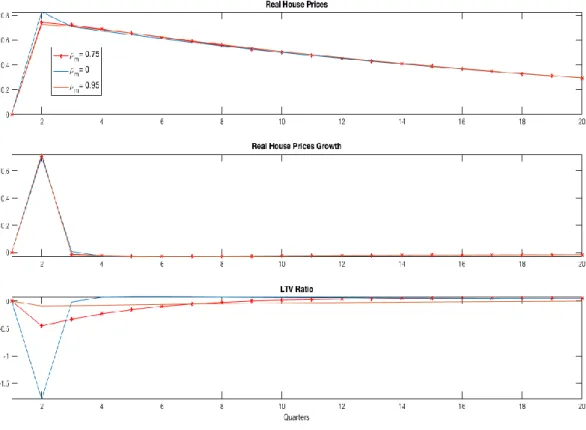
Alternative calibrations of the persistence parameter term (𝜌𝑀= 0, 0.3, 0.95). The charts for the IRFs will display the following variables: consumption for both types of households, borrowing of impatient households, real consumption, real business
investment, real residential investment, real house prices, nominal interest rate, inflation, LTV ratio, house prices growth and, in the last case, also credit growth.
4.2 Housing Preference Shock
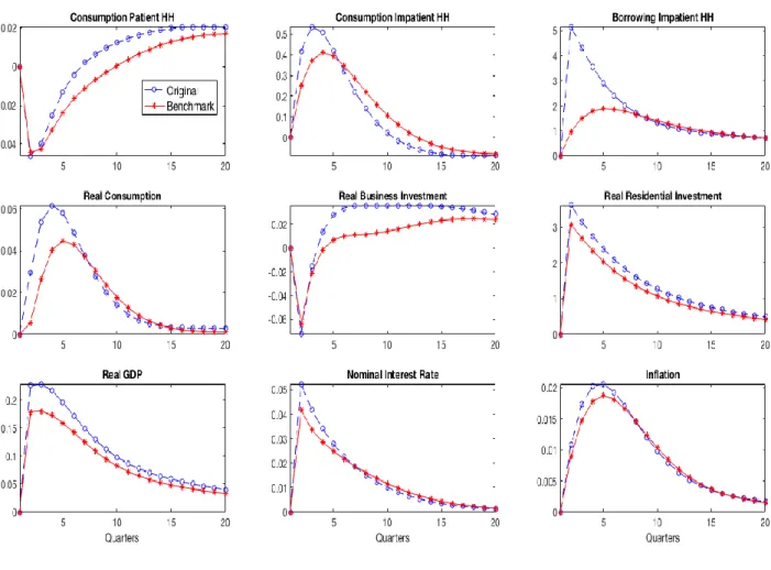
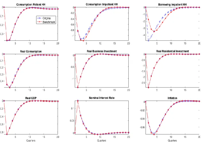
Figures 1-2 show the IRFs to a transitory one standard deviation housing preference shock.34 The shock represents an interesting way to analyse how systematic macroprudential policy impacts the transmission mechanism of shocks, since this shock directly affects the demand for housing that is the asset used as collateral in the model. Two specifications of the model are considered, i.e. the “Original” and the “Benchmark” as described above.
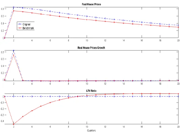
Focusing on the model with a constant LTV ratio (the “Original” setup), as consequence of the (positive) housing preference shock, the demand for housing increases leading to a rise in house prices and residential investment (because agents receive higher returns from this sector). Impatient households can borrow more given the increase in the value of their collateral, which allows them to consume more. Patient households increase lending to impatient ones and invest more in the housing sector, thus transferring resources away from consumption that drops on impact. Given the increased demand for housing, investment in this sector rises and so the capital stock in this sector increases. Since there is a shift in resources towards the residential sector, capital in the consumption sector drops, thus business investment falls. The combined effect of an increase in aggregate consumption and these opposing dynamics in the two types of investment drive an increase in GDP and in inflation, requiring the central bank to tighten monetary policy. Focusing now in the case when the LTV ratio responds according to the benchmark rule, given that a housing preference shock generates an increase in house prices, the macroprudential authority responds by decreasing the LTV ratio. This constrains the borrowing capacity of impatient households, containing borrowing. On impact, real house prices are also contained by the response of the macroprudential authority. Consumption of impatient agents thus increases to a lower extent and, consequently, also aggregate consumption. The main difference in terms of macroeconomic outcomes is in the behaviour of consumption, as would be expected given that the macroprudential instrument is the LTV ratio of borrowers, i.e. impatient consumers.
Results of this simulation show that having the macroprudential authority reacting to house price growth mitigates the effects of the shock. Given that the macroprudential authority counteracts the macroeconomic expansion (leaded by an increase in house prices and borrowing), the monetary policy response does not have to be as strong as in the “Original” setting, as in the “Benchmark” case the macroprudential policy and monetary policy authorities perform in a complementary way.
Figure 1: Housing Preference Shock - Original vs Benchmark 35
35 The y-axis measures percent deviation from the steady state (inflation and nominal interest rate are
Figure 2: Housing Preference Shock – Original vs Benchmark – House Prices and LTV Ratio 36
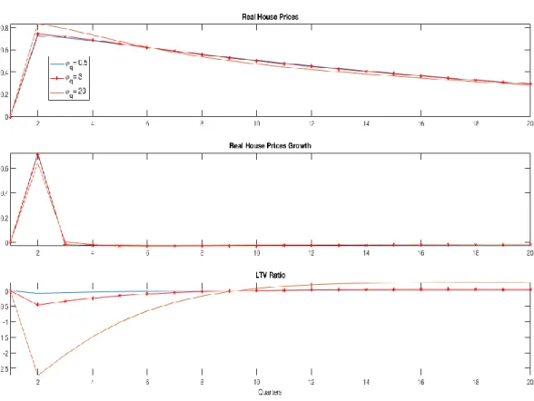
For the same shock, Figures 3-4 display the IRFs sensitivity analysis regarding the parameter controlling the macroprudential authority response to house prices growth (∅𝑞𝑀).
Higher (lower) values of the parameter compared to the benchmark (∅𝑞𝑀 = 3) correspond to a stronger (smaller) reduction of the LTV ratio by the macroprudential authority, as illustrated in Figures 3-4 for two extreme cases.
A smaller value of ∅𝑞𝑀 compared to the “Benchmark” case leads to a smaller reduction in the LTV ratio following the shock. Therefore, impatient households are less constrained to borrow (compared to the “Benchmark” case) and consequently consumption increases slightly more.
Higher values of ∅𝑞𝑀 imply a greater reduction in the LTV ratio. We take as an example a situation where the macroprudential authority is much more reactive than in the benchmark rule (i.e. ∅𝑞𝑀= 20). Following the shock, the LTV ratio falls
36 In this figure (and all similar figures in this section), the y-axis measures percent deviation from the
steady state in the case of house prices and percentage point deviations in the case of house price growth and LTV.