Numerical Modelling of Subcooled Boiling Flow based on Mechanistic Approach: A Validation Study using Wet Steam (IAPWS) as Working Fluid Properties

Numerical Modelling of Subcooled Boiling Flow based

on Mechanistic Approach: A Validation Study using

Wet Steam (IAPWS) as Working Fluid Properties

Machimontorn Promtong, Sherman C.P. Cheung, Jiyuan Tu

Abstract—Due to the safety conditions for operating the nuclear reactors, a number of researches have attempted to gain more knowledge and to understand the boiling flow phenomena. In this research, the wall boiling models, based on the mechanistic approach, were improved into ANSYS CFX 14.5 for studying the sub-cooled boiling flow. Basically, these constituted models are required for predicting the main parameters at the heated wall boundary, which include (i) nucleation site density, (ii) bubble departure diameter, and (iii) bubble departure frequency. Currently, the wall heat flux partitioning closures have been modified to consider an influence of bubble sliding along the wall before the lift-off, which usually happens in the flow boiling. For the simulation, it was performed based on the Two-fluid model, together with the k-ɛ turbulent model. Also, the properties of Wet Steam (IAPWS) at considered temperature and pressure operations were adopted as the working fluid conditions. The available experimental data, which observed the boiling flow at the low pressure, were chosen. The results showed that the void fraction, vapor velocity, liquid velocity, and Sauter Mean Diameter (SMD) from the predictions were found to be in fair agreement with the experiments. Thus, the current mechanistic models are necessary to develop further to obtain more accurate prediction of this flow. According to the experimental works, the mechanisms, such as a merging of bubbles during sliding, a shrinking of bubbles during the condensation, will be considered for the code development in the future work.

Index Terms—Two-fluid model; Subcooled boiling flow; Wall partitioning heat flux; Bubble interactions; Mechanistic model; Population balance method; Computational Fluid Dynamics (CFD)

I. INTRODUCTION

Sub-cooled boiling flow is of the most interest to nuclear power industries because it presents typical nuclear reactors

Machimontorn Promtong is a PhD student in school of Aerospace, Manufacturing and Mechanical Engineering (SAMME), RMIT University, Melbourne, VIC 3083 Australia (corresponding author - phone: +61(0)42364-5352; e-mail: machimontorn.promtong@rmit.edu.au).

Sherman C.P. Cheung is a Associate Professor in school of Aerospace, Manufacturing and Mechanical Engineering (SAMME), RMIT University, Melbourne, VIC 3083 Australia (e-mail: chipok.cheung@rmit.edu.au).

Jiyuan Tu is a Professor in school of Aerospace, Manufacturing and Mechanical Engineering (SAMME), RMIT University, Melbourne, VIC 3083 Australia (e-mail: jiyuan.tu@rmit.edu.au).

and plays a key role in cooling of the reactor core. Due to the safety operation and new designs of the nuclear reactors, many researchers have attempted to gain more understanding in sub-cooled boiling flow phenomena. In general, the size of vapor bubbles, which are nucleated from the heat wall, can represent a portion of latent heat from the heated wall carried into the bulk liquid. However, other important parameters, including a bubble growth rate (frequency) and a waiting time during the bubble generation, are also needed to be considered. This is because they can determine how fast energy is transferred to the liquid. Basically, these boiling parameters are involved in determining the boiling heat flux partitions; convective, quenching and evaporative heat flux. Based on intensively investigated experimental studies, they have been formulated in the forms of empirical correlations [1], [2] and [3].

In the past decades, there have been a number of experimental works studying the pool boiling and the flow boiling [4], [5], [6], [7], [8] and [9]. These significant works allow us to develop and improve an accuracy of the numerical techniques in predicting the boiling phenomena. Afterward, some confidential models have been adopted into Computational Fluid Dynamics (CFD) software for predicting the boiling application [10], [11], [12] and [13]. For instance, the

RPI (Rensselaer Polytechnic Institute) model which is

available in ANSYS CFX is used to predict the pool boiling [14]. However, to introduce this RPI algorithm for predicting the flow boiling, the available consituted models used to predict bubble departure diameter, nucleation site density and bubble frequency, have to be modified to account more realistic bubble behaviors which happen in a forced convective sub-cooled boiling flow. For example, the experimental observation suggested that there has been a sliding of bubbles before their departures [15], [16] and [17]. Recently, there has been an attempt to experimentally study the sliding bubble dynamics to gain a better understanding of the boiling heat transfer mechanism [18].

evaluate the accuracy of the proposed models in term of predictions this flow behavior.

The objectives of this work were (i) to evaluate the current mechanistic approach in term of the prediction accuracy for studying the sub-cooled flow boiling, and (ii) to address a further development of the current employed models in order to extend a wider range prediction of this flow. In order to assess the modeling accuracy, the results i.e. bubble size distribution, void fraction distribution, temperatures and velocities of liquid and gas were compared with the experimental data.

II. FLOW DESCRIPTIONS AND GOVERNING EQUATIONS

A. Phenomenological descriptions

Flow characteristic of the sub-cooled boiling is presented in Fig. 1a. Basically, the sub-cooled liquid flows pass through the heated wall, and then vapor bubbles start to initiate on the wall at the ONB (Onset of Nucleate Boiling). The location where the amount of vapor starts to significantly increase is called the Net Vapor Generation (NVG), in which the sub-cooling temperature is dominant the flow structure.

From Fig. 1b, the void fraction of vapor gas may increase along the way because of bubble interactions including the break-up and the coalescence. In contrast, the size of vapor bubble may be reduced because of condensation, when they leave the wall and oppose to the lower- temperature bulk liquid.

B. Two-fluid model

Computational Fluid Dynamics (CFD) method of two-phase flow systems relies on the average flow models, and they may range from simple mixture models to more complex two-fluid models [13, 21, 22]where the equations are separately solved for each individual phase. Physically, this flow can be also described based on the averaged equations of continuity, momentum and energy governing of

each phase. For the gas phase, it is represented as disperse phase (

g

 ), and its ensemble-averaged equation is written as follows:

- Continuity equation of gas phase:

(1)

For the liquid phase, the liquid is represented as the continuum phase (_l), and their continuity is written as:

- Continuity equation of liquid phase:

(2)

Where



is the density,



is the volume fraction,

u



is the velocity vector. It should be noted that the right term of the equations (



lg) is involved in the calculation because of the condensation effect.

The momentum equations of gas and liquid phases are expressed as follows:

- Momentum equation of liquid phase:

(3)

- Momentum equation of gas phase:

(4)

Where e

l



and



_ge are the effective viscosities of the liquid and gas phases, respectively. These viscosity terms are calculated using the turbulence models which are normally required since the nature of this forced convective sub-cooled boiling is turbulent.

- Interfacial momentum forces:

The total interfacial force

F

lg in equations (3) and (4) is formulated based on the appropriate consideration of different sub-forces affecting the interface between each phase. For the liquid phase, the total interfacial force is given by the drag, lift, wall lubrication, and turbulent dispersion, and they are shown in equation (5). More details regarding these terms can be found from the work of Anglart and Nylund [23].

(5)





_Γlg

   

 g g _{g g g}

u

α ρ

t

α

ρ 

fg l sat if

h ) T (T a

h 

 

lg lg ;



ρ α u u



α P α ρ g t

u α

ρ g g g g g g g

g g g

 

 

    

   

lg lg

F ug_



 





_Γlg

   

 l l _{l l l}

u

α ρ

t

α

ρ 

lg lg

F ul 



 



ρα uu



α P α ρ g t

u

α

ρ l l l l l l l

l l l

 

 

    

   

 







e l lT



l l

u u

α   

  

 







e g gT



g

g

u u α   

 

dispersion lg rication lub lg lift lg drag lg

lg F F F F

F    

(a) (b)

Fig. 1. Phenomenological descriptions of subcooled boiling flow;

Since the gas phase was assumed to be at saturated situation, the calculating requirement of energy equation of gas phase was ignored. The energy equation of liquid phase may be expressed as:

- Energy equation of liquid phase:

(6)

Equation (7) expresses a calculation of the interfacial heat transfer (

lg

Q) term at the energy equation, and in this case it

represents the heat transfer due to the condensation process.

- Interfacial energy terms:

(7)

In order to calculate the heat transfer at the interface, the interfacial area term (a_if) is necessary, and as displayed in equation (7), it can be calculate based on the bubble mean diameter (D_s) and gas void fraction (



_g).

C. Population Balance Method

Population Balance Methods (PBM) is widely used as a co-operation with the multi-fluid modeling framework to determine the coalescence and break-up phenomena of bubbles. Recently, the performance of different PBM including direct quadrature method of moments (DQMOM) [24], average bubble number density (ABND) model [25], and MUlti-SIze-Group (MUSIG) model [26], has been assessed.

In this simulation, Inhomogeneous Multiple-Size-Group (MUSIG) model, originally developed by Lo [26], was adopted to account a non-uniform bubble size distribution. The bubbles were divided into 15 classes of equal diameter, and each class was traveled at different velocities.



g j i j



ji i ph i

i j j

R

m

S

u

f

α

ρ

t

f

α

ρ

)

(

,















_

(8)

Where the source term (S_j,_i) of this equation is a

representative of the birth and dead rates caused by the coalescence and breakage of bubbles. To obtain these terms, the model proposed by Luo and Svendsen [27] was employed for calculating the break-up rate , and the model proposed by Prince and Blanch [28] was adopted for calculating the coalescence rate. The details of them are not descried here. For the second term (

ph

R ) on the right of the

equation, it represents the source rate due to phase change, and this can represent the mass transfer due to the condensation.

III. THE CONSTITUTED MODELS FOR THE WALL HEAT FLUX

PARTITIONING ALGORITHM

In order to obtain the parameters required for the wall heat-flux partitioning algorithm, the constituted models employed for nucleation site density, bubble departure diameter and bubble lift-off frequency calculations are detailed as follows:

- Nucleation site density (N_a)

For the nucleation site density calculation, the fractal analysis, originally formulated by Mikic and Rosenow [29], was employed in this study. Basically, this model considers the nucleation site density based on a power correlation of the active cavities on heated surface. As presented in equations (8), (9), (10) and (11), the variables including the superheat temperature (

sup

T ) and the sub-cooling

temperature (T_sub) and the liquid properties, which are required for thermal boundary thickness (_l) calculation, are mainly participated in this model.

(8)                  ) ( 4 2 sup 3 2 sup sup 1 min , T C T T T T C D sub sub l c _   ₍₉₎                  ) ( 4 2 sup 3 2 sup sup 1 max , T C T T T T C D sub sub l c

_





(10) min , max , 2 min , max , ln 2 1 ln c c c c f D D D D d                 

(11)

From the above equations, D_c,maxand D_c,minare the maximum and minimum of active cavity diameter. The

d

_f

term represents the area fractal dimension (1<

d

_f <2) and

 is the contact angle of the fluid on the heated wall. Where   2T_sat /_gh_fg, C1(1cos)/sin and

  1 cos

3

C . Further details regarding the fractal analysis can be found from Yun et al. [19].

- Bubble lif-off diameter(D_l)

For the bubble lift-off diameter calculation, the force balance approach, formulated by Klausner et. al [15] and Zeng et. al [30], was introduced in this study. All the forces acting at the vapor bubbles are depicted in Fig. 2, and the equations used for calculating the bubble diameter are shown in (12) and (13). Basically, the bubble lift-off diameter (D_l) can be obtained when a summation of the







e l





gl l l



l l l l l l l l l H H Q T α H u α ρ t H α

ρ _{   } lg_{  }lg

   ) T (T a h

Qlg lg if g l ;aif 6g D_s



 i i i s d f D 1 ; f d c ,max

a c ,min c c ,max

c

D

N D D D

D

 

_{ }  

forces involved in the x-direction (perpendicular to the wall) is equal to zero





Fx _0



. Similarly, for the y-direction,

several forces are involved in calculating a size of the sliding bubble (D_sl).This sliding diameter can be obtained when the summation of forces reach a zero





Fy _0



. It

should be noted that this value is required for calculating the bubble influence area for the quenching heat flux term.

- Along the x-direction:



F

_x



F

_sx



F

_dux



F

_sL



F

_h



F

_cp (12)



cos _r cos _a



;

r a w sx d

F  

 



 

 



; cos i du dux F

F 



;

2

1_{C U}2 _r2

F_sL  _L



_l



; 4 4

9 2 w2 l

h

d U

F 







r w cp

r d F



2



4

2



- Along the y-direction:



F

y



F

sy



F

duy



F

qs



F

b (13)



sin sin



; )

( ) (

2

2 a r

r a

r a w

sx d

F  

  

  

 

 

 



; sin _i

du duy F

F 



F 6C U r;

l D qs 







; ) (

3 4 3

g r

F_b 





_l



_g

Where

F

_sx

,

F

_sy are the surface tension forces;

duy dux

F

F

,

are the unsteady drag forces due to asymmetrical growth of the bubble;

F

_sL is the shear lift force;

F

_h is the force due to the hydrodynamic pressure;

cp

F

is the contact pressure force accounting for the bubble being in contact with a solid;

F

_qs is the quasi steady-drag force in the flow direction; and

F

_b is the buoyancy force.

Also,



_a,



_rand



_i are the advancing, receding and inclination angles, respectively;

d

_w is surface/bubble contact diameter;

g

is gravitational acceleration;

r

is the bubble radius and



U

is the relative velocity between bubble and the liquid;

C

_Dand

C

_Lare drag and lift force coefficients, respectively; and their formula has been found in Klausner’s work [15].

- Bubble lift-off frequency (f)

In this study, the bubble frequency term was calculated using a mechanistic approach proposed by Yeoh et al. Basically, this frequency term is formulated by considering a life cycle of vapor bubble generation at the active cavity site. By substituting the waiting time and the growth time, the formula for bubble lift-off frequency can be obtained as follow:

g w

t

t

f





1

(14)

The consuming time after the departure of a vapor bubble from the cavity site (or waiting time) and just before the regeneration of a new vapor bubble (quenching time) can be estimated by using Hsu’s criteria, and it can be expressed as follow:





2

2 sup

1 sup

/ 2 1

    

  

  

c fg g sat

c sub w

r h C T T

r C T T t







(15)

Where

T

_sup is the wall superheat and

T

_sub is the sub-cooled temperature;

C

₁



(

1



cos



)

/

sin



and



sin / 1

2

C , r_c is the cavity radius; and



is the liquid thermal diffusivity. For further details regarding the equation, it can be found from Yeoh [1]. For the term of the growth time (

t

_g), it is examined by adopting the sliding diameter (D_sl) into (16).

2 2

2

16 1

Ja b

D

t sl

g

_





(16)

    

   

fg g

l l

h T k Ja





_sup

(17)

Where Ja is represented as a Jacob number and it may be estimated from the above equation.

Fig. 2. Schematic diagram of the forces acting on a vapor bubble

IV. EXPERIMENTAL DESCRIPTIONS

Three cases from an experimental study of Lee [20] were introduced in this validation study. The operation details of each case are presented in the Table 1. Noticeably, the wall heat flux and liquid mass flux for each case are different, and the operating pressures for all cases are at low pressure. Working fluid used in the experimental study was demineralized water. Moreover, the uncertainties of the void fraction, liquid and gas velocities were 3% and the bubble Satuter Mean Diameter was 27%.

Table 1. Experimental details of the flow conditions of the selected cases

Case Pinlet

(kPa) Tinlet

(°C)

Tsat-Tinlet

(°C)

Qwall (kW/m2)

G (kg/m2s)

L1 142 96.6 13.4 152.3 474.0

L2 137 94.9 13.8 197.2 714.4

L3 143 92.1 17.9 251.5 1059.2

As shown in the Fig. 2, the experimental configuration of Lee consists of a vertical concentric annulus with an inner heating rod of 19 mm outer diameter. The length of heated section is 1.67 m. This rod can produce a uniform heat using a 54kW DC power supply. The diameter of outer wall is 37.4 mm, and there is a transparent glass connected for visual observation. The measuring plane for collecting the experimental data is 1.61 m, and this is far from the inlet as depicted in the Figure.

V. SIMULATION DETAILS

Two sets of continuity, momentum, energy of each phase were simultaneously solved based on the finite volume method. Since the gas phase was assumed to be a saturated condition, this could lead to only one energy equation for the liquid phase. The SIMPLE algorithm was used to handle the coupling of velocity-pressure calculation. Again, the Inhomogenous MUSIG was employed to track the bubble size distribution. Thus, the iterative process the fifteen transport equations were coupled with the flow equations.

Because of annular geometrical shape, only a quarter of the annulus could be considered in this simulation. The total grid, used in calculation, was 1170, with 13(radial) x 30(height) x 3(circumference). The operating conditions, such as wall heat fluxes, mass flux, sub-cooling temperatures from Lee’s experiments, were adopted into the simulations as the boundary and initial conditions.

Also, to gain more realistic simulation, the properties of Wet Steam (IAPWS-IF97) at the considered ranges of temperature and pressure were used as the working fluid conditions. So far, no standard turbulence model has been tailored for bubbly flow in handling bubble induced turbulent flow. However, because the void fraction of this flow was considerably low and the bubble sizes were relatively small, the standard k–ε model was adopted for the liquid phase and dispersed phase zero-equation was employed for the gas phase.

For boiling model, the proposed models, which consist of the fractal model (2002), the force balance model (1993), and the mechanistic model (2008), were examined through a CFD code. These proposed closures were implemented into the commercial Computational Fluid Dynamics (CFD) code named ANSYS CFX 14.5 via user FORTRAN files. Usually, at each equation of the size fraction (except at the smallest group, Group 1), additional source terms should be accounted for the condensation effects; however these terms have not been implemented into the current simulation yet. However, at the heated wall boundary the nucleation terms were included into the size fraction equations of the groups which have the mean diameter closed to the bubble lift-off diameter as the evaporative heat sources.

Overall, the convergences of all the simulation cases were found between 4200 and 6500 iterations when their residual terms were below 1x10-6. The total times consumed for all simulation cases for their calculations were less than 5 hrs.

VI. RESULTS AND DISCUSSIONS

A. Void fraction

The prediction of local mean radial profiles of void fraction comparing with the experiments is presented in Fig. 3. Among these three cases, the highest void fraction was similarly shown at near the heated wall; this may be a result of lots of bubble nucleated from the heat wall. However, when it was far away from the wall, the void fraction was decreased, and this reduction may be due to the condensation. As we known, when the departed bubbles opposed to the bulk liquid which has lower temperature, the sizes of them became smaller. Hence, it was also resulted in lower void fraction. For the case L152, the predicted void

fraction was higher than the experiment, and this may be caused by an over-prediction of a portion of the evaporative heat flux from the wall heat flux.

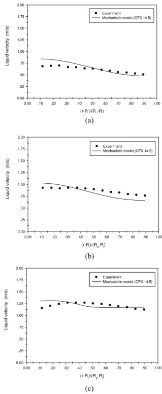
B. Liquid velocity

As shown in Fig. 4, at near the heated wall, the predicted velocities of case L152 and case L197 were higher than the experiment, and the lower values were found at the locations far from the wall. This may be a result of high temperature at the heat wall. However, for the case L252, the highest velocity from the experiment was found at the middle of the

flow channel instead. Since this case had the highest of the mass flux comparing with the others, thus the velocity field may be dominated by this high flow-rate, and it may also be less influenced by the wall temperature if compared with the other cases. Among these cases, similar trend were found between the predictions and experiments, and the differences between them were less than 0.20 m/s.

(r-R_i)/(R_o-R_i)

0.00 .10 .20 .30 .40 .50 .60 .70 .80 .90 1.00

Li

q

u

id

v

e

lo

ci

ty

(m

/s)

0.00 .25 .50 .75 1.00 1.25 1.50 1.75 2.00

Experiment

Mechanistic model (CFX 14.5)

(r-R_i)/(R_o-R_i)

0.00 .10 .20 .30 .40 .50 .60 .70 .80 .90 1.00

L

iqui

d v

el

ocit

y

(m/

s

)

0.00 .25 .50 .75 1.00 1.25 1.50 1.75 2.00

Experiment

Mechanistic model (CFX 14.5)

(r-R_i)/(R_o-R_i)

0.00 .10 .20 .30 .40 .50 .60 .70 .80 .90 1.00

L

iqui

d v

el

oc

it

y

(m/

s

)

0.00 .25 .50 .75 1.00 1.25 1.50 1.75 2.00

Experiment

Mechanistic model (CFX 14.5)

Fig. 4. Comparisons of local mean radial profiles of liquid velocity between experiment and prediction; (a) Case L152, (b) Case L197,

(c) Case L252

(r-Ri)/(Ro-Ri)

0.00 .10 .20 .30 .40 .50 .60 .70 .80 .90 1.00

V

o

id

fr

ac

ti

o

n

(



)

0.00 .10 .20 .30 .40 .50 .60 .70 .80 .90 1.00

Experiment

Mechanistic model (CFX 14.5)

(r-Ri)/(Ro-Ri)

0.00 .10 .20 .30 .40 .50 .60 .70 .80 .90 1.00

Vo

id

fra

c

ti

o

n

(



)

0.00 .10 .20 .30 .40 .50 .60 .70 .80 .90 1.00

Experiment

Mechnistic model (CFX 14.5)

(r-R_i)/(R_o-R_i)

0.00 .10 .20 .30 .40 .50 .60 .70 .80 .90 1.00

V

o

id

f

ractio

n

(



)

0.00 .10 .20 .30 .40 .50 .60 .70 .80 .90 1.00

Experiment

Mechanistic model (CFX 14.5)

Fig. 3. Comparisons of local mean radial profiles of void fraction between experiment and prediction; (a) Case L152, (b) Case L197,

(c) Case L252

(a)

(b)

(c) (a)

(b)

C. Gas velocity

From Fig. 5, the local mean radial profiles of predicted vapor velocities of case L152 and case L197 were in a similar trend. Their gas velocities closed to the heated rod were slightly higher than the experimental results. This may be because the sizes of bubbles on that area are smaller than the bubble size from the experiment, then it could result in higher velocities. However, in the reality, while the flowing-up, the travelling bubbles may merge/collide to the neighbors, those are still attached the heated rod. Eventually, they become bigger bubbles and result in lower vapor velocities at the area closed to the heated rod.

For the case L252, the predicted velocity of vapor was similar with the others, as higher velocity than the experiment was found at near the heated surface. Interestingly, there was a sudden drop of the vapor velocity at the locations far from the heated rod, and this could imply that there were no flowing bubbles at that locations. Overall, the vapor velocities of all cases were higher than the liquid velocities, as a result of lighter density (buoyancy force) of the vapor.

D. SauterMean Diameter (SMD)

The comparisons between the predictions of the mean bubble diameter and the experiments at the measuring plane are shown in Fig. 6.

(r-R_i)/(R_o-R_i)

0.00 .10 .20 .30 .40 .50 .60 .70 .80 .90 1.00

Vapor

v

eloc

it

y

(m/s

)

0.00 .25 .50 .75 1.00 1.25 1.50 1.75 2.00

Experiment

Mechanistic model (CFX 14.5)

(r-R_i)/(R_o-R_i)

0.00 .10 .20 .30 .40 .50 .60 .70 .80 .90 1.00

V

a

p

o

r v

e

lo

c

ity

(

m

/s

)

0.00 .25 .50 .75 1.00 1.25 1.50 1.75 2.00

Experiment

Mechanistic model (CFX 14.5)

(r-R_i)/(R_o-R_i)

0.00 .10 .20 .30 .40 .50 .60 .70 .80 .90 1.00

Va

po

r v

e

loc

ity

(m/s

)

0.00 .25 .50 .75 1.00 1.25 1.50 1.75 2.00

Experiment

Mechanistic model (CFX 14.5)

Fig. 5. The comparisons of local mean radial profiles of vapor velocity between experiment and prediction; (a) Case L152,

(b) Case L197, (c) Case L252

(r-Ri)/(Ro-Ri)

0.00 .10 .20 .30 .40 .50 .60 .70 .80 .90 1.00

Bu

bbl

e saut

er

m

ean d

iam

e

te

r (

m

m

)

0.00 .50 1.00 1.50 2.00 2.50 3.00 3.50 4.00 4.50 5.00 5.50 6.00

Experiment

Mechanistic model (CFX 14.5)

(r-Ri)/(Ro-Ri)

0.00 .10 .20 .30 .40 .50 .60 .70 .80 .90 1.00

Bu

bbl

e saut

er

m

ean d

iam

e

te

r (

m

m

)

0.00 .50 1.00 1.50 2.00 2.50 3.00 3.50 4.00 4.50 5.00 5.50 6.00

Experiment

Mechanistic model (CFX 14.5)

(r-Ri)/(Ro-Ri)

0.00 .10 .20 .30 .40 .50 .60 .70 .80 .90 1.00

Bu

bbl

e saut

er

m

ean d

iam

e

te

r (

m

m

)

0.00 .50 1.00 1.50 2.00 2.50 3.00 3.50 4.00 4.50 5.00 5.50 6.00

Experiment

Mechanistic model (CFX 14.5)

Fig. 6. Comparisons of local mean radial profiles of SMD between experiment and prediction; (a) Case L152, (b) Case L197,

(c) Case L252

(a)

(b)

(c)

(a)

(b)

From the experimental results, the bubbles which were near the wall were usually big, and their size was getting smaller following the longer distance from the wall. Once bubbles leave the wall, they will be opposed to the bulk liquid which has lower temperature. Then, the heat and mass from the bubbles are transferred to the bulk liquid (condensation), as shown from the Figures, their sizes become smaller and they can be disappeared.

However, from the prediction, the bubble sizes which are far from the wall were slightly smaller than those close to the heated wall. Also, the predicted mean sizes of bubbles closed to the heated rod were smaller than the experimental results. In contrast, the bigger sizes comparing with the experiments were located far from the head rod. Thus, this can show a significant difference between the current predicting results and experiments.

As mentioned earlier, the condensation effects at the PBM equations of the simulations have not yet been considered. Thus, the effect from condensation process cannot be clearly observed from the predictions. Therefore, a further work regarding about the condensation terms is required to gain more accurate simulation.

E. Simulation results regarding the boiling model

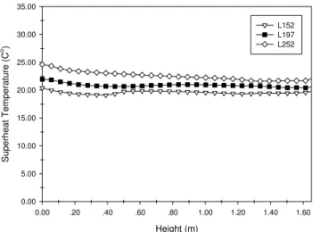
As shown in Fig. 7, the highest wall temperature from the predictions was about 17.5 °C (case L252), and it was as low as 12.5 °C for the case L152. This can be explained by comparing the heat flux among these three cases (Table 7.1). The case L252 showed the highest heat flux, therefore, the predicted results were higher than the others. Moreover, among the cases, the wall superheat temperature which was near the inlet was higher than the other area; apart from that the temperature remained nearly constant along the height.

From Fig. 8, the predicted results of nucleation site density from three cases were between 1.0-2.8 millions per m2. At the near inlet, the values are at lower values, and this may be because they are affected from high sub-cooling temperature. Usually, the nucleation site density will increase following the amount of the superheat temperature. So, the value from the case L252 should be higher than that

from the case L152. However, this is not happened in this study and this may be because the liquid mass fluxes and their sub-cooling temperature of the cases are also different.

According to the fractal analysis, not only the superheat temperature was considered for predicting the nucleation site density, but the sub-cooling temperatures and other liquid properties were also involved. Thus, the higher nucleation site density was found when the superheat temperature was high and the sub-cooling temperature was low. However, for the case of L252, the mass flux was high (higher liquid velocity), resulting in the slightly reduced sub-cooling temperature when compared with the other two cases (which have lower liquid velocities at the inlet). Therefore, even though the case L252 showed a higher superheat temperature (Fig. 7), there may be higher sub-cooling temperature as well. Therefore, based on the fractal model, the L252 case could be resulted in lower number of nucleation site density, as shown in the Fig. 8. Furthermore, it can be noticed a sudden change of the nucleation site density for the case L152 (Fig. 8), and this may be because from that location the fluid temperature become more stable.

As depicted in Fig. 9., the predicted bubble lift-off frequency of all the cases based on the mechanistic approach was between 50-80 Hz. Normally, the predictions of bubble

Height (m)

0.00 .20 .40 .60 .80 1.00 1.20 1.40 1.60

S

u

pe

rh

ea

t T

e

m

p

e

rat

ure

(C

o)

0.00 5.00 10.00 15.00 20.00 25.00 30.00 35.00

L152 L197 L252

Fig. 7. Predicted wall superheat temperatures on the heated surface along the

height of the rod

Height (m)

0.00 .20 .40 .60 .80 1.00 1.20 1.40 1.60

N

u

clea

ti

o

n

si

te

de

n

s

o

ity

(1

/m

2)

0.00 5.00e+5 1.00e+6 1.50e+6 2.00e+6 2.50e+6 3.00e+6 3.50e+6 4.00e+6

L152 L197 L252

Fig. 8. Predicted nucleation site density on the heated surface along the

height of the rod

Height (m)

0.00 .20 .40 .60 .80 1.00 1.20 1.40 1.60

Bubble lif

t-off

freq

uenc

y

(

1

/s

)

0 10 20 30 40 50 60 70 80 90 100 110 120

L152 L197 L252

Fig. 9. Predicted bubble frequency on the heated surface along the height of

frequency of the case which has a lower heat flux should present lower value. However, for the case of L152 which has the lowest of heat flux, it represented at the highest frequency for a certain distance from the inlet. Moreover, its frequency was reduced to be below the other cases after 0.40 m of the height above the inlet. From further investigation, it was found that at that height the bubble lift-off diameter was suddenly changed to have bigger sizes, as a result of higher level of the force interactions. Finally, the longer time was required before its lifting-off and this was consequently resulted in lower frequency which is mechanistically calculated using the bubble growth time and the waiting time.

VII. CONCLUSION AND FUTURE WORK

The wall boiling closures including the fractal model, the force balance approach, and the bubble frequency have been successfully implemented into the ANSYS CFX 14.5 for studying the subcooled boiling flow. Based on the present mechanistic approach, the prediction results were in reasonable agreements with the experimental data. As we know, the properties of Wet Stream are changed following the conditions of pressure and temperature, thus using them as the working fluid in the simulations; some realistic mechanisms of subcooled boiling flow could be observed. Regarding the bubble size distribution, the current Inhomogenous MUSIG method may require a further modification to include the condensation term at the bubble size equations to increase the prediction accuracy. As a result, the void fractions of the cases, except Case L197, were higher than the experiments. This can be a result of high prediction of partitioning evaporative heat at the wall boiling algorithm. In another word, the proposed closures may give the over-predicted values of the area influenced by the vapor bubbles and/or the bubble lift-off diameter. Thus, our attentions for future work will be directly toward to the development of the force balance approach, i.e. the micro-layer evaporation, the condensation at the bubble tips and bubble merging during sliding. This way could eventually improve a better prediction of the heat partitioning from the heated wall and also could increase an accuracy prediction of the flow structure variables, for example, the void fraction and the bubble distribution.

ACKNOWLEDGMENT

The financial support provided by the Australian Research Council (ARC project ID DPXXXXXXXX) is gratefully acknowledged.

REFERENCES

[1] Yeoh, G.H., et al., Fundamental consideration of wall heat partition of vertical subcooled boiling flows. International Journal of Heat and Mass Transfer, 2008. 51(15-16): p. 3840-3853.

[2] Warrier, G.R. and V.K. Dhir, Heat Transfer and Wall Heat Flux

Partitioning During Subcooled Flow Nucleate Boiling—A Review.

Journal of Heat Transfer, 2006. 128(12): p. 1243.

[3] Basu, N., G.R. Warrier, and V.K. Dhir, Wall Heat Flux Partitioning During Subcooled Flow Boiling: Part 1—Model Development.

Journal of Heat Transfer, 2005. 127(2): p. 131.

[4] Cooper, M.G., The microlayer and bubble growth in nucleate pool

boiling. International Journal of Heat and Mass Transfer, 1969.

12(8): p. 915-933.

[5] Yang, C., et al., Study on bubble dynamics for pool nucleate boiling.

International Journal of Heat and Mass Transfer, 2000. 43(2): p. 203-208.

[6] Levy, S., Forced convection subcooled boiling—prediction of vapor volumetric fraction. International Journal of Heat and Mass Transfer, 1967. 10(7): p. 951-965.

[7] Rogers, J.T., et al., The onset of significant void in up-flow boiling of water at low pressure and velocities. International Journal of Heat and Mass Transfer, 1987. 30(11): p. 2247-2260.

[8] Thorncroft, G.E., J.F. Klausner, and R. Mei, An experimental

investigation of bubble growth and detachment in vertical upflow and downflow boiling. International Journal of Heat and Mass Transfer, 1998. 41(23): p. 3857-3871.

[9] Basu, N., G.R. Warrier, and V.K. Dhir, Onset of Nucleate Boiling and Active Nucleation Site Density During Subcooled Flow Boiling.

Journal of Heat Transfer, 2002. 124(4): p. 717-728.

[10] Tu, J.Y. and G.H. Yeoh, On numerical modelling of low-pressure

subcooled boiling flows. International Journal of Heat and Mass Transfer, 2002. 45(6): p. 1197-1209.

[11] Yeoh, G.H. and J.Y. Tu, A unified model considering force balances for departing vapour bubbles and population balance in subcooled boiling flow. Nuclear Engineering and Design, 2005. 235(10-12): p. 1251-1265.

[12] Kocamustafaogullari, G. and M. Ishii, Interfacial Area and

Nucleation Site Density in Boiling Systems. International Journal of Heat and Mass Transfer, 1983. 26(9): p. 1377-1387.

[13] Ishii, M., Interfacial Area Modeling. 1987. 3: p. 31-62.

[14] Kurul, N.a.P., M. Z.,, On the modeling of multidimensional effects in boiling channels. ANS Proc. 27th National Heat Transfer Conference, Minneapolis, MN,, 1991.

[15] Klausner, J.F., et al., Vapor Bubble Departure in

Forced-Convection Boiling. International Journal of Heat and Mass Transfer, 1993. 36(3): p. 651-662.

[16] Situ, R., et al., Bubble lift-off size in forced convective subcooled boiling flow. International Journal of Heat and Mass Transfer, 2005.

48(25-26): p. 5536-5548.

[17] Cho, Y.-J., et al., Development of bubble departure and lift-off diameter models in low heat flux and low flow velocity conditions.

International Journal of Heat and Mass Transfer, 2011. 54(15-16): p. 3234-3244.

[18] Xu, J., et al., Experimental visualization of sliding bubble dynamics in a vertical narrow rectangular channel. Nuclear Engineering and Design, 2013. 261: p. 156-164.

[19] Yu, B. and P. Cheng, A Fractal Model for Nucleate Pool Boiling

Heat Transfer. Journal of Heat Transfer, 2002. 124(6): p. 1117. [20] Lee, T.H., G.C. Park, and D.J. Lee, Local flow characteristics of

subcooled boiling flow of water in a vertical concentric annulus.

International Journal of Multiphase Flow, 2002. 28(8): p. 1351-1368. [21] Zhang, D.Z. and A. Prosperetti, Ensemble phase‐averaged equations for bubbly flows. Physics of Fluids (1994-present), 1994. 6(9): p. 2956-2970.

[22] A. Prosperetti and G. Tryggvason, Computational Methods for

Multiphase Flow. Cambridge Univ. Press, 2007.

[23] Anglart, H. and O. Nylund, CFD application to prediction of void distribution in two-phase bubbly flows in rod bundles. Nuclear Engineering and Design, 1996. 163(1–2): p. 81-98.

[24] Marchisio, D.L. and R.O. Fox, Solution of population balance

equations using the direct quadrature method of moments. Journal of Aerosol Science, 2005. 36(1): p. 43-73.

[25] Duan, X.Y., et al., Gas–liquid flows in medium and large vertical pipes. Chemical Engineering Science, 2011. 66(5): p. 872-883.

[26] Lo, S. and A. Technology, Application of Population Balance to

CFD Modeling of Bubbly Flow Via the MUSIG Model. 1996. [27] Luo, H. and H.F. Svendsen, Theoretical model for drop and bubble

breakup in turbulent dispersions. AIChE Journal, 1996. 42(5): p. 1225-1233.

[28] Prince, M.J. and H.W. Blanch, Bubble coalescence and break-up in air-sparged bubble columns. AIChE Journal, 1990. 36(10): p. 1485-1499.

[29] MIKIC, B.B., A new correlation of pool-boiling data including the effect of heating surface characteristics. Journal of Heat Transfer, 1969.

[30] Zeng, L.Z., et al., A unified model for the prediction of bubble detachment diameters in boiling systems—II. Flow boiling.

International Journal of Heat and Mass Transfer, 1993. 36(9): p. 2271-2279.

[31] Gerardi, C., et al., Study of bubble growth in water pool boiling through synchronized, infrared thermometry and high-speed video.