Feedback-control operators for improved Pareto-set description:
Application to a polymer extrusion process
Eduardo G. Carrano
a, Dayanne Gouveia Coelho
b, António Gaspar-Cunha
c, Elizabeth F. Wanner
d,
Ricardo H.C. Takahashi
e,naDepartment of Electrical Engineering, Universidade Federal de Minas Gerais, Brazil bDepartment of Computing, Universidade Federal de Ouro Preto, Brazil
cInstitute for Polymer and Composites
–I3N, University of Minho, Campus de Azurém, 4800-058 Guimarães, Portugal dDepartment of Computing, Centro Federal de Educação Tecnológica de Minas Gerais, Brazil
eDepartment of Mathematics, Universidade Federal de Minas Gerais, Brazil
a r t i c l e
i n f o
Article history:
Received 4 September 2013 Received in revised form 7 July 2014
Accepted 21 October 2014 Available online 26 November 2014 Keywords:
Evolutionary computation Multiobjective optimization Genetic algorithms Polymer extrusion Local search
a b s t r a c t
This paper presents a new class of operators for multiobjective evolutionary algorithms that are inspired on feedback-control techniques. The proposed operators, thearchive-set reductionand thesurface-filling crossover, have the purpose of enhancing the quality of the description of the Pareto-set in multi-objective optimization problems. They act on the Pareto-estimate sample set, performing operations that eliminate archive points in the most crowded regions, and generate new points in the less populated regions, leading to a dynamic equilibrium that tends to generate a uniform sampling of the efficient solution set. The internal parameters of those operators are coordinated by feedback-control inspired techniques, which ensure that the desired equilibrium is attained. Numerical experiments in some benchmark problems and in a real problem of optimization of a single screw extrusion system for polymer processing show that the proposed methodology is able to generate more detailed descriptions of Pareto-optimal fronts than the ones produced by usual algorithms.
&2014 Elsevier Ltd. All rights reserved.
1. Introduction
One of the main concerns in the design of multi-objective evolutionary algorithms (MOEAs) has been to ensure the quality of the sample set of Pareto-optimal estimates that is generated by the algorithm. The quality measure is, by itself, multi-dimensional,
and there are not, up to now, any definitive standards that
represent it (Zitzler et al., 2003; Auger et al., 2012). A
high-quality solution set can be defined as a set of samples that reach,
as long as possible, the exact Pareto-set, and is representative of
the whole extension of the Pareto-set (Silva et al., 2007; Zitzler et
al., 2010). It should be noticed that a MOEA can be built with the purpose of describing a subset of the Pareto set, in the cases in
which some a priori or online decision information is available
(Kim et al., 2012; Sinha et al., 2013). In those cases, the quality
measures should refer to the representation of such subsets (Auger
et al., 2012).
This paper introduces new operators that can be used to enhance the ability of a MOEA to represent the Pareto set in
detail, with a uniform spread of the samples: the sphere-control
operators. Such operators are based on the information about the
distances between every pair of solution samples in a set –this
motivates the denomination of“sphere”operators. The key idea is
the usage of afeedback-controlinspired scheme (Ogata, 2001) in
order to establish a dynamic equilibrium along the algorithm iterations, associated to the high-quality description of the Pareto-set. While such a high-quality description is not reached, some measured variables do not reach an equilibrium, causing a control action that will enhance a quality metric.
The proposed methodology is applied to an optimization problem of the operational and screw geometrical parameters of a single screw polymer extrusion system. In this problem, a modeling routine describing properly the complex process developed is necessary. This involves the mathematical description of the different phases
suf-fered by the polymer inside the machine (Gaspar-Cunha, 2009). This
practical problem of strong industrial relevance concerns the employment of multiobjective optimization on a simulation model
for the purpose of gaining knowledge about possible efficient
operating modes to be implemented in a real machine. The main purpose of such a multiobjective optimization study is to obtain
Contents lists available atScienceDirect
journal homepage:www.elsevier.com/locate/engappai
Engineering Applications of Arti
fi
cial Intelligence
http://dx.doi.org/10.1016/j.engappai.2014.10.016 0952-1976/&2014 Elsevier Ltd. All rights reserved.
n
Corresponding author.
E-mail addresses:[email protected](E.G. Carrano),
selecting the best operating conditions and/or screw geometry. Further discussions about the application of evolutionary computa-tion methods for problems in materials science and engineering are
reported inPaszkowicz (2013).
An instance of application of a feedback-control inspired
scheme, as proposed here, is represented inFig. 1. In thisfigure,
the measured variable is the error e¼q a, which feeds a
mechanism that is inspired in the proportional-integral (PI) controller, which in turn determines the value of the control
variable
ρ.
ρ, which represents the radius of the spheres associated
to the points in the archivefile, plays the role of the control input
variable, while the variable a, which represents the number of
points in the archivefile, plays the role of the controlled variable. The pre-established reference number of points in the archive,
denoted byq, will be attained in an equilibrium1situation that will
be reached due to the feedback mechanism.
In the equilibrium, e¼0 (which means the desired result of
a¼q). As in other contexts of application of feedback-control techniques, the role of the feedback-control inspired scheme here is to induce an overall system behavior that presents low sensi-tivity to variations in the initial conditions and in the algorithm parameter values, delivering stable results, with repeatability in
the reach of high-quality solution sets (Ogata, 2001). The error
variables are defined here such that the feedback loop reaches an
equilibrium only when a good description of the Pareto-set is attained.
Specifically, two sphere-control operators are presented here:
an archive-set reductionoperator, which controls the number of non-dominated solutions that are stored, and a crossover operator that is applied in the archive set, thesurface-filling crossover. The archive-set reduction plays the role of solution density reduction
in the most crowded regions of the Pareto-set. The surface-filling
crossover is to be applied in the less crowded regions of the
Pareto-set, in order to fill eventual gaps in its description. The
equilibrium between the opposite actions of surface-filling and
archive-reduction, attained by a feedback-control inspired scheme, leads to an ultimate description of the Pareto-set that is composed of samples that are evenly distributed in the space of objectives.
Feedback-control inspired mechanisms, based on the principles of a switched controller and of a proportional-integral (PI)
con-troller, are employed in the surface-filling operators and in the
archive-set reduction operator, in order to enhance the distribu-tion of soludistribu-tions along the Pareto surface. This motivates the
denomination of“sphere-control”operators. These operators are
to be employed together, since their effects are complementary, and their dynamic interaction is necessary in order to achieve the desired behavior.
It should be noticed here that the idea of feedback-control inspiration constitutes a further step beyond some studies that
have considered the theme ofparameter adaptationin
evolution-ary computation. Examples of those studies can be found for
andSilva et al. (2007)which employ“sphere” operations which are similar to the archive-set reduction operator presented here, yet without any feedback adaptation scheme.
The basic idea, both in that references and here, is that a
“sphere”means roughly a domain in which the information gained
by a solution point in its center would be representative–with no
need of further function evaluations inside such a sphere.Bui et al.
(2008, 2009)also employ the concept of“spheres” for construc-tion of an MOEA (multi-objective evoluconstruc-tionary algorithm), with a
dual meaning: in that cases, the“sphere”is the domain in which a
local search is conducted, with sub-populations assigned to per-form searches inside each sphere.
In the specific formulation that is presented here, the proposed
operators are structured for continuous-variable spaces. However, the adaptation for discrete-variable problems can be performed
directly, provided that some distance metric becomes defined in
the discrete-variable space. This can be performed according to the
guidelines presented byCarrano et al. (2010).
It should be noticed that the proposed methodology may be supplemented by the usage of local search operators, that can enhance the precision of solutions if applied along the algorithm
iterations (Wanner et al., 2008), or even provide a certificate of
optimality in some cases (Takahashi et al., 2011). Those
hybridiza-tions are not discussed further, in order to privilege the presenta-tion of the main aspects of the methodology proposed here.
This paper is structured as follows. A discussion about
multi-objective evolutionary algorithms is provided in Section 2. The
proposed feedback-control inspired operators are presented in
Section 4. Section 3presents a modified version of the classical NSGA-II algorithm, in which the proposed sphere-control opera-tors are included. The results of numerical tests on some
bench-mark problems are presented inSection 5. The numerical tests
show that the proposed methodology leads to a significant
enhancement of the ability of the algorithm for reaching afi
ne-grained description of the Pareto-optimal set. Finally, inSection 7, the proposed algorithm is employed in the problem of polymer extrusion process design. The results are compared with the ones obtained using the basic NSGA-II and with another algorithm, the RPSGA, that was employed formerly for dealing with the same problem. The results support the conclusion that the proposed
methodology is able to significantly enhance the description of the
efficient solution set in this practical problem too.
2. Multiobjective evolutionary algorithms
Consider fðÞ:Rn↦Rm a vector-valued real function. Let fiðÞ
denote thei-th coordinate of the function in the image space. The
multiobjective problems appear from the partial ordering induced
by the relation ofdominance:
u!v3
fiðuÞrfiðvÞ 8i¼1;…;m and
(iAf1;…;mgsuch thatfiðuÞofiðvÞ 8
> <
> :
ð1Þ
Consider the Pareto-setPdefined by
P9fxn
A
Ω
j∄xAΩ
such thatx!xng ð2Þin whichxARn is the decision variable vector, and
Ω
DRnis thefeasible set. A multiobjective optimization problem is defined as
the task of generating samples of the set P. A multiobjective
evolutionary algorithm (MOEA) is an evolutionary algorithm
which is intended to produce a set of samples ofP. At the end
of the execution, the archive setAkcontains the algorithm
out-come, which constitutes an estimate of the Pareto-setP.
3. MOEA with sphere-control operators
This paper presents new evolutionary operators which are not
intended to be algorithm-specific. Instead, they should be suitable
to be inserted in any MOEA that works with archive solutions. For this reason, in this paper the proposed operators are inserted within a standard MOEA, the Non-Dominated Sorting Genetic
Algorithm II (NSGA-II) (Deb et al., 2002), in order to define a
working algorithm. The resulting algorithm, named Sphere-Control Multiobjective Genetic Algorithm (SCMGA), is compared here with the basic NSGA-II over a set of benchmark problems, in
order to establish somefigures about the effect of introducing the
sphere-control operators inside a known MOEA. The basic NSGA-II
and the proposed SCMGA are described briefly in this section.
3.1. The NSGA-II
The Non-dominated Sorting Genetic Algorithm (Deb et al.,
2002), or simply NSGA-II, has been used for dealing with the
multiobjective optimization problems considered here. For a full description of that algorithm, the reader should refer to the original reference. The following procedures, which are part of NSGA-II, will be employed in the next section in the construction of the SCMGA (the Sphere-Control Multiobjective Genetic Algorithm):
A’non_dominatedðPÞ returns the individuals that lie in thefirst front of the populationP;
F’fast_non_dominated_sortingðPÞ sorts the individuals of population according to fronts, the solutions in each front dominated only by solutions in the former ones; Ci’crowding_distance_assignmentðFiÞ employs a crowding distance assignmentprocedure to estimate how the solutions offrontiare spread in the objective space;
Q’selectionðP;NÞ uses binary stochastic tournaments withreplacement for performing selection of a new populationQ,
composed ofNindividuals, from populationP.
3.2. The SCMGA
The structure of the Sphere-Control Multiobjective Genetic Algorithm (SCMGA), is similar to the one of the original NSGA-II. Basically, this algorithm presents three major differences in rela-tion to the original one:
Archive size control scheme: In the original NSGA-II, an elitist selection scheme allows the current population to serve as an archive, which is built upon the crowding distance measure. However, while the control of the archive size based on crowd-ing distance is efficient for two objectives, it is not so reliablewhen more objective functions are considered (Kukkonen and
Deb, 2006). In the proposed algorithm, an external archive uses
the sphere-based archive control procedure (Section 4.1). The PI
controller that is used for performing the archive-size control
adjusts the radius
ρ
in order to keep theqmost representativesolutions (or a number of solutions that is close to q). As this
method employs spheres for controlling the archive size, it is suitable for dealing with any number of objective functions, since spheres can be fully parametrized by the radius only, in spaces of any dimension. The archive, in SCMGA, interacts with the population on the end of each iteration.
Insertion of surface-filling crossover: The surface-fillingcross-over, described in Section 4.2, is executed at the end of each
iteration in order to fill the blank spaces of the archive. The
number of surface-filling crossover operations which are
per-formed depends on the measured efficiency of this operator in
the previous generations.
Auto-adaptation of the algorithm parameters: The controllerparameters
ρ,
β
and rare adjusted inside the SCMGA. Theρ
parameter is adjusted based on the current number of solutions
in the archive and the desired one. The
β
parameter is adjustedin order to obtain solutions which are not excessively near the
parents in surface-filling crossover. Finally, therparameter is
adjusted based on the efficiency of surface-filling crossover: if the number of successful operations is higher than the
unsuc-cessful onesrdecreases; otherwiserincreases.
The details of these operations are described in the next
section. Algorithm 1 shows the pseudo-code for the SCMGA
algorithm.
Algorithm 1. Pseudocode for SCMGA.
Inputs:N,q ▹N: population size;
q: archive size
Output:A ▹A: archive set
t’0
ρ
;β
;r’start_ρ_β_rPt’new_populationðNÞ ▹generates random
population of size N Qt’∅
A’non_dominatedðPtÞ whilenot stop criteriondo
Rt’Pt[Qt
F’fast_non_dominated_
sortingðRtÞ
Ptþ1’∅
i’1
whilejPtþ1jþjFijrNdo
Ci’crowding_distance_
assignmentðFiÞ Ptþ1’Pt[Fi i’iþ1 end while
Fi’sortðFi;Ci;‘descending’Þ ▹sorts fronti, descending order ofCi Ptþ1’Ptþ1[Fi½1:ðN jPtþ1jÞ
Qtþ1’selectionðPtþ1;NÞ Qtþ1’crossoverðQtþ1Þ Qtþ1’mutationðQtþ1Þ t’tþ1
A’non_dominatedðA[QtÞ
ðT;k1;k2;k3;k4;k5;k6Þ ’Surf_Fill_XOðA;
ρ
;r;4;β
Þ ðr;β
Þ’Update_r_βðr;
β
;k1;k2;k3;k4;k5;k6ÞQt’Qt[T
upper bounds respectively.
4. The sphere operators
Consider the setsAandPrespectively meaning the archive and
the current population:
A9fx1~ ;…;xa~ g
P9fx1;…;xpg ð3Þ
withjAj ¼aandjPj ¼p. The images of such sets in the objective space are denoted by
Ay¼ fy~ 1;…;y~
ag9ffðx1~ Þ;…;fðxa~ Þg
Py¼ fy1;…;ypg9ffðx1Þ;…;fðxpÞg ð4Þ
In this paper it is considered that both setsAyandPyare
normal-ized between 0 and 1, according to extreme values ofAy(0 and
1 are assigned to the minimum and maximal value in each dimension respectively). These sets are re-normalized every time
Ayis updated.
The main idea which is behind the “sphere operators” is to
enhance representativity of the archive Aby evaluating its
reg-ularity. If the solution samples regularly cover the set P, they
should be located in relation to their nearest neighbors such that the distances to them become of the same order of magnitude.
Therefore, a parameter
ρ, which has the meaning of a
referencedomain radiusfor each point, must be defined.
This parameter is employed in order to guide the algorithm operations, with the intent to generate points which
approxi-mately “represent” the region inside the sphere of such radius
centered in that point. Any two neighbors should be separated, therefore, by at least 2ρ. In the regions in which the points are too densely distributed, an operation of decimation should be per-formed. In the regions in which the points are too sparsely distributed, new solution points should be found and included in the archive. The indication of what operation should be performed in each region is obtained via the comparison of the distances
between the points with this parameter. The parameter
ρ
isdynamically adjusted during the algorithm execution, in order to reach a good dispersion of the sample points along the Pareto-set estimate, considering a reference value of the number of sample points that is to be found.
The sphere-control operators to be presented in this section are: (i) the archive size control, and (ii) the surface-filling
cross-over. The surface filling mutation operator should also be
men-tioned, presented inTakahashi et al. (2009), which is not discussed
in detail here. The effect of those operators is illustrated inFig. 2.
4.1. Archive size control
Consider the set A¼ fx1;x2;…;xm;xmþ1;…;xag in which the
individual minima of themobjective functions have been put in
thefirst mpositions, and the remaindera mpoints have been
ordered randomly. The set Ay is ordered correspondingly. The
archive set size is controlled byAlgorithm 2. After this operation,
there will be no two points inAywith pairwise distances smaller
Ay’Ay fyjjJyi yjJo
ρ
;iajg i’iþ1end while
Algorithm 3.Pseudocode for
ρ
Control [Update_ρ].Inputs:A;q;
ρ
Output:
ρ
Parameters:s;Kp;Kn a’jAj
ifa4qthen e’ða qÞ=q
ife4sthen
Δ
’Kps elseΔ
’Kpe end ifρ
’ð1þΔ
Þρ
else
ρ
’Knρ
end ifIf this operation was executed with a pre-defined value of
ρ,
this could cause the sizeaof setAto become too large or too small,
since the exact extension of the setPis not knowna priori. On the
other hand, the number of efficient solutions which are kept in the
archive is a variable that can be measured easily, and this
information can be used in order to adjust
ρ, in order to reach a
coverage of the setPwith a“resolution”
ρ.
The adjustment of parameter
ρ
takes into account a referencenumber of points that should be stored in the archive setA. Let
such a reference number be denoted by q, and let a¼ jAj. The
adjustment procedure is described inAlgorithm 3. Default values
can be indicated for the control parameters: Kp¼0.6, s¼0.1,
Kn¼0.9. The initial value of
ρ
is defined such that qspheres ofdimension ðm 1Þ occupy a volume equivalent to the unitary
simplex of dimensionðm 1Þ.
Algorithm 3performs the adjustment of the value of
ρ
in thefollowing way. If the reference number of pointsqis greater than
the current number of points in the archive,a, then the value of
ρ
should be increased, in order to decrease the archive size. The
percentage increase in
ρ
is given byΔ.
Δ
is calculated as a constantKp times the relative error e betweena and q. However, if e is
greater than a thresholds, the value of
Δ
is saturated asKptimesthis thresholds. This saturation is introduced in order to avoid a
very fast change in the value of
ρ, which could cause oscillations in
the number a of points in the archive, possibly harming its
convergence.
On the other hand, if the reference number of points q is
smaller than the numberaof points in the archive, then
ρ
shouldbe decreased, in order to cause the archive size to increase. For the
purpose of this reduction in
ρ, a constant factor
Knis employed,instead of employing a factor proportional to the relative errore.
first steps of the algorithm, when the number of archive solutions
is much smaller than the reference numberq, and also causes a
small step decrease of
ρ
on any time that a decrease becomesnecessary when the system is near the equilibrium. A diagram of
such a closed-loop feedback control scheme is presented inFig. 1.
This algorithm resembles the PI (proportional-integral) controllers with control signal saturation, which are employed in industrial control systems.
It should be noticed that, as the control action over variable
ρ
isincremental, the net effect has the form of anintegralcontrol. This
integral term in the PI controller is necessary in order to induce an error-less steady behavior in the closed-loop system. Indeed, if a
simple P(proportional only) controller were adopted, the steady
state value of the controlled variableawould not become equal to
the reference valueq. Explaining this point: consider the situation in
which there is a positive error between aand q, meaning that
ρ
should be increased in order to make that error decrease. If the value
of
ρ
was itself proportional to the errorethen there would be avalue of that error that, when multiplied by the constantKp, would
give rise to a value of
ρ
which would cause exactly that value oferror to appear–causing an equilibrium situation that would not
lead to further error reductions. However, if the value of the errore is used to calculate an increment
Δ
proportional to it, by adding thisincrement to the value of
ρ
will make the value ofρ
to alwaysincrease for any positivee, eventually leading the erroreto converge to zero. In this way, the PI controller structure is the simplest one
that fulfills the requirement of producing exactlyaevenly spaced
solutions (most textbooks on classic control theory, for instance
Ogata (2001), will present a detailed discussion about such effects). The adoption of such a closed-loop control scheme makes the
size of
ρ
to reach an equilibrium point by itself, avoiding the needof ana prioriknowledge about such a parameter, and rendering
the multiobjective genetic algorithm robust in relation to this parameter. Notice that even in the degenerate case of the
Pareto-set surface being of dimension less than m 1 (one or more
objectives being redundant), the algorithm still works as expected,
forming an archive set of Pareto estimates which will still haveq
evenly spaced elements.
4.2. Surface-filling crossover
Define the functionvðÞas
vðyiÞ ¼ jfyjjJyi yjJo3ρgj ð5Þ
which means the cardinality of the set of points from the archive
set Ay which is inside a ball of radius 3ρ around the function
argumentyj. Without loss of generality, consider that the setAyis
ordered in increasing order ofvðyiÞ:
Ay¼ fyijvðyiÞrvðyiþ1Þg ð6Þ
The set Areceives the corresponding ordering, andjAj ¼a. After
receiving the ordering as defined by(6), the archiveAbecomes
arranged in such a way that thefirst solutions are the ones which
have less neighbors in the objective space.
The parameter r, which is between 0 and 1, represents the
proportion of elements in archive that will be submitted to the surface-filling crossover(SFXO) operation. This parameter is one of the control variables that will be adjusted dynamically by
Algorithm 5. The r jAj first solutions of A (after sorting) are chosen to perform the SFXO. The ordering is chosen such that a
random solution is initially chosen to be the first parent p1.
Afterward, the solution which is nearest to the current parentpi
is chosen, among the solutions which have not been selected yet. In the end, the procedure delivers a set of parentsfp1;p2;…;prjAjg which will suffer crossover. The SFXO will perform the crossover operations of (p1 vs. p2), (p2 vs. p3), (p3 vs. p4), …, (pðrjAj 1Þ vs. prjAj). Therefore,r jAj 1 crossover operations are performed each
time. The SFXO operator is defined inAlgorithm 4.
Algorithm 4. Pseudocode for SFXO [Surf_Fill_XO].
Inputs:A ▹archive set
Inputs:r,
β
▹controlled parametersOutputs:T,F ▹set of enhanced
solutions (decision and objective space)
k1;k2;k3;k4;k5;k6’0
T;F’∅
p’Sequence_SFXOðA;rÞ fori¼1 toðr jAj 1Þdo
b¼Betað
α
;β
Þ^
xi’ð1 bÞ piþbpiþ1 ^
yi’fðxi^Þ
vf’FALSE ifJy^
i fðpiÞJo
ρ
thenk5’k5þ1
vf’TRUE end if
if Jy^i fðpiþ1ÞJo
ρ
thenk6’k6þ1
vf’TRUE end if ify^
i!fðpiÞory^i!fðpiþ1Þthen
k1’k1þ1
T’T [xi^
F’F[y^i
else ify^
igfðpiÞory^igfðpiþ1Þ
then
k2’k2þ1 Else
ifvf¼FALSEthen if∄jjfðAjÞ!yi^ then
k3’k3þ1
T’T [xi^
F’F[y^i
else
k4’k4þ1 end if end if end if end for
In this algorithm, the command p’Sequence_SFXOðA;rÞ
returns the sequence of parents fp1;p2;…;prjAjg on which the SFXO operator will be executed.
The main idea of the SFXO is to interpolate solutions which have less neighbors in the objective space (i.e., less other points at a distance smaller than 3ρ). These individuals are subjected to
crossovers which are intended tofill the gaps on the archive set, in
order to generate a better description of the Pareto set. The
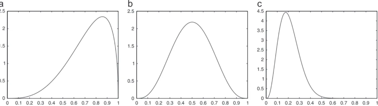
parameter
α
of the Beta distribution has been kept fixed inα
¼4, in order to generate concave probability distributionfunctions (PDFs). On the other hand, the parameter
β
hasbeen modeled as a controlled variable, which can vary dynami-cally inside the algorithm in order to adjust the Beta
distribu-tion: lower values of
β
lead the median of the PDF to approach1 and higher values of Beta lead the median of the PDF to approach
0. The variable
β
therefore can be used to approximate theoffspring solution to either p1 or p2. The shapes of the PDF
of Beta distribution for
α
¼4 and different values ofβ
areshown inFig. 3. Each new solution obtained by thesurface-filling
crossover is analyzed, with the results driving the following counters:
Counterk1: xi^ dominatespiorpiþ1; Counterk2: xi^ is dominated bypiorpiþ1;
Counterk3: xi^ is not dominated by neither pi, piþ1 nor by any
other solution inA;
Counterk4: xi^ is not dominated by neitherpinorpiþ1, but it is
dominated by some other solution inA;
Counterk5: The distance betweenxi^ andpiis lower than
ρ;
Counterk6: The distance betweenxi^ andpiþ1is lower than
ρ.
This means that the counterkiis increased each time a solution makes the respective condition to become true. These six counters are used to estimate the efficiency of the operator and to updaterandβ
values.The pseudo-code forrand
β
tuning is shown inAlgorithm 5.Algorithm 5. Pseudocode forrand
β
control in SFXO [Update_r_β].Inputs:r,
β
▹controlled parametersInputs:k1;k2;k3;k4;k5;k6 ▹counters used for parameter adaptation
Outputs:r,
β
bexp’log10ðβ
Þ rinv’1rnSFXO’k1þk2þk3þk4 ▹number of SFXO operations performed SSFXO’k1þk3 ▹number of successful SFXO operations USFXO’k2þk4 ▹number of unsuccessful SFXO operations
ifk5Z0:25nSFXOork6Z0:25
nSFXOthen
▹
β
controlifk54k6then
bexp’0:90bexp ▹approach the median top2
else
bexp’1:10bexp ▹approach the median top1
end if end if
ifSSFXOZUSFXOthen ▹rcontrol
rinv’0:90rinv ▹increase the number of
SFXO operations
else
rinv’1:10rinv ▹decrease the number of
SFXO operations
end if
ifbexpo0:25then ▹
β
controller saturation-lower bound bexp’0:25
else ifbexp41:25then ▹
β
controller saturation -upper bound bexp’1:25end if
ifrinv410then ▹rcontroller saturation
-lower bound rinv’10
else ifrinvo2then ▹rcontroller saturation -upper bound rinv’2
end if
r’r1
inv
β
’10bexpThe parameters
β
and rare updated according to the resultsobserved in SFXO operations:
When a significant part (more than 25%) of the offspringsolutions are concentrated near p1, the Beta distribution is
adjusted in such a way that, in next generation, the operator will have higher chance of generating solutions which are more far away from it. The same holds for the case ofp2. In this way, the operator tends to generate new solutions which are located not too close to any parent solution.
When the SFXO presents more successful than unsuccessfulcases in one generation, the number of expected crossover operators is increased for the next iteration. On the other hand, when more unsuccessful operations are performed this num-ber is decreased.
The adjustment of variables is always performed in small steps, by increasing or reducing 10% of the current value. This is adopted in order to avoid abrupt variations which could cause instability in the algorithm. Both controllers also have lower and upper bounds in the control action.
After the execution of SFXO, all the solutions which are not
dominated by any solution ofAand whose distance top1andp2
are higher than
ρ
are delivered by the SFXO as a setT, which isinserted in the populationQ of the GA, in order to improve the
quality of the current population.
Assuming that solutions which are near on the parameter space are usually not so far away on the objective space, it is reasonable
to admit that a crossover operation would be suitable forfilling the
blank spaces within archive, performing the interpolation of
solutions. It should be noticed that the surface-filling crossover
operator is likely to generate new points that are located nearby the same manifold in which the parent points lie. This means that, especially in the case of Pareto-set manifolds of relatively low dimension embedded in high-dimensional decision variable
spaces, the surface-filling crossover tends to be efficient in the
task of finding new Pareto-optimal points. Indeed, in the tests
conducted within this study, the surface-filling crossover has been
found to be more efficient than the surface-filling mutation which
was proposed inTakahashi et al. (2009). Due to this, the
surface-filling mutation has not been considered in the present work.
4.3. Time complexity
With regard to computational complexity, the procedure employed to perform archive size control is built upon three
major (and more costly) operations: (i) extreme solution identifi
-cation: before performing archive size control, it is necessary to identify the extreme points of the current Pareto-front approx-imation, in order to ensure that these points are not displaced
during the operator execution. It can be performed inOðjAjÞtime,
in which A is the archive that stores the current Pareto-set
approximation; (ii) solution distance evaluation: the archive size control algorithm requires that the distances between all points in the archive are known. It is possible to accomplish such a calculation in OðjAj2Þ time; (iii) Paretofiltering: the while-loop ofAlgorithm 2can, in the worst case, compare each solution with
all thejAj 1 remaining ones. Therefore, the execution of such a
loop is bounded toOðjAj2Þtime complexity.
Since these three operations are the most costly in the procedure, it is possible to conclude that the archive size control
can be executed in OðjAj2Þ time. It should be noticed that the
desired number of solutions in the archive is a user-defined
parameter and, therefore, it is not affected neither by the problem dimension nor by the number of objectives.
The SFXO2executes, for ar
jAj number of times, a crossover
operator that is, usually, very similar to the one employed in the original algorithm. Therefore, the complexity of the SFXO can be
estimated as r jAj times the computational complexity of the
crossover operator. Since the size of jAj is controlled, and r is
bounded by a maximum value, the SFXO computational complex-ity is then controlled by the algorithm parameters.
However, it must be emphasized that, in most part of cases, the function evaluations are the main responsible for the algorithm processing time. In those cases, the additional time required to perform SFXO calculations (excluding function evaluation) could
be ignored, since it would be insignificant when compared to the
time required to evaluate the solutions generated by the operator itself. The number of solutions evaluated inside SFXO is counted as normal algorithm evaluations, in order to keep algorithm com-parisons fair.
5. Numerical tests
In order to assess the suitability of the proposed methodology, a series of numerical tests has been conducted over a set of 18 benchmark functions. The description of those benchmark multi-objective optimization problems is presented in the Appendix.
In order to support the comparisons, the NSGA-II implementa-tion found in PISA (Zitzler, 2010) has been translated to Matlab 7,3 in order to be used as benchmark. This algorithm employs exactly the same operators (simulated binary crossover and polynomial
mutation, Deb and Agrawal, 1995) and structure of the original
one. Such as in the PISA implementation, the probability distribu-tion funcdistribu-tion of the operators are adjusted in order to generate real values only in the intervalf0;1g. A scheme that controls the size of the archive has been included in order to keep it at a
pre-defined size. This scheme is based on the crowding distance
assignment, and it is referred ascrowding_archive_reductionin
Section 3.1.
2The complexity of the procedure adopted to adjustρandβis not discussed here because it requiresOð1Þtime.
This algorithm has been used also as the basis for the implementation of the sphere-control hybrid algorithm presented in this paper (SCMGA). In the SCMGA, the control of the archive size is performed using
ρ_
Archive_Control(Section 4.1) instead ofcrowding_archive_reduction. The surfacefilling crossover is also
executed at each algorithm generation, as shown inAlgorithm 1.
The procedures that adjust
ρ,
β
and r are also executed in theSCMGA variant.
The performances of these two algorithms on the benchmark problems considered here have been compared in order to estimate the effect of the sphere-control operators on the algo-rithm convergence. The performances of the algoalgo-rithms, in each test problem, are compared through the following steps:
Performance comparison procedure.
1. Each algorithm is executedktimes for the same parameter set
and stop criterion;
2. Based on the minimum and maximum values achieved for each objective, considering all algorithms and runs, normalize the fronts between 0 and 1 (the values 0 or 1 are not necessarily present on each Pareto-front approximation);
3. For each runiof thekruns:
(a) Join the archive obtained by the original NSGA-II (ANSGA IIi )
and the archive obtained by the SCMGA (ASCMGA
i ) into a
single archiveA;
(b) Perform dominance on A and create A0 with the
non-dominated points ofA;
(c) MakeA0NSGA IIi ¼ANSGA IIi \A0andASCMGAi ¼A0SCMGAi \A0;
(d) Employ some Pareto quality metricPQMfor evaluating the
convergence performances of the NSGA-II and SCMGA algorithms:
qNSGA II
i ¼PQMðA
0NSGA IIi;A0SCMGA
i Þ;
qSCMGA
i ¼PQMðA0SCMGAi ;A0NSGAi IIÞ.
4. Sort theqNSGA IIandqSCMGAvectors in ascending order.
This process returns k quantiles associated with the
conver-gence performance of the algorithms that are being considered. These quantiles can be used for performing a stochastic
dom-inance analysis, as discussed in Carrano et al. (2010). From the
stochastic dominance principle, it is possible to say that a
multi-objective algorithmA1stochastically dominates another algorithm
A2(A1gA2) if, and only if
A1gA2: qA1
i Zq
A2
i 8iA1;…;k
(ijqA1
i 4q
A2 i 8
<
:
ð7Þ
Therefore,A1 dominatesA2 if allkquantiles ofA1 are higher or
equal the quantiles ofA2and at least one quantile ofA1is higher
than the same quantile ofA2. This kind of analysis provides an
accurate comparison of the algorithm outcomes.
Although this process is considerably better than single run comparison or visual analysis, it still has a problem: for a moderate number of algorithm executions, the order in which the archives
are compared can effect the vectorsq, because the result of the
dominance analysis is dependent on the sets that are being compared. This order dependence can give rise to inaccurate results, since two different executions of the proposed scheme could lead to different (or even opposite) results. In order to avoid this inconvenient, permutation test procedures have been used for performing algorithm analysis. In each permutation test, random permutations of the indexes of the archives obtained by the algorithms are generated. The archives are compared following such indexes, and the process is repeated for a pre-determined
number of times P. Each permutation test provides a set of
quantilesqfor each algorithm. Thefinal value of the quantileqi
is obtained by determining the median of allPvalues assigned to
the quantile qi in the permutation tests. This procedure avoids
order biasing of the solutions, and reduces the variability between the responses provided by the method when comparing the same algorithms.
5.1. Pareto quality metrics
In this paper, three Pareto quality metrics (PQM) have been used to estimate the quality of the Pareto approximations
deliv-ered by the algorithm: the C metric (Zitzler and Thiele, 1998) for
set coverage, the
Δ
metric (Deb et al., 2002) for set spacing and theintegrated sphere counting metric (Silva et al., 2007), which tries
to handle with both aspects at once.
C Metric (CM): The C metric, proposed byZitzler and Thiele (1998), estimates the coverage of two Pareto set approximations,
based on the dominance principle. LetX be the set of candidate
decision vectors for a given problem and letADX,BDX be any
two sets of decision vectors. The coverage ofAwith regard toB,
CðA;BÞ, can be evaluated as follows:
CðA;BÞ ¼jfaAAj(bAB:b⪯agj
jAj ð8Þ
In this expression, the fraction gives the ratio of solutions fromA
that are dominated by solutions fromB. IfCðA;BÞ ¼0, thenAdoes
not have any dominated solutions when compared toB; on the
other hand, ifCðA;BÞ ¼1, then all solutions ofAare dominated by
at least one solution ofB. In this way, a lower value ofCmeans a
more suitable Pareto front approximation.
Δ
Metric(Δ
M): TheΔ
metric, proposed byDeb et al. (2002), is used to estimate how the solutions of the approximated Pareto-setare spaced into the objective domain. LetXbe the set of candidate
decision vectors for a given problem and letADX be any set of
decision vectors. The
Δ
metric forA,Δ
ðAÞ, can be calculated asfollows:
Δ
ðAÞ ¼∑ mi¼1d
e
iþ∑j
Aj
i¼1jdi dj
∑m
i¼1d
e
iþjAj d
ð9Þ
in whichmis the number of objectives;dieis the Euclidean distance
between the extreme points in A and in Xn
; diis the Euclidean
distance between the point iAA and its closest neighbor, in the
objective space;dis the average of all distancesdi; andXn
is the real Pareto set of the problem. From(9), it is straightforward to note that
lower values of
Δ
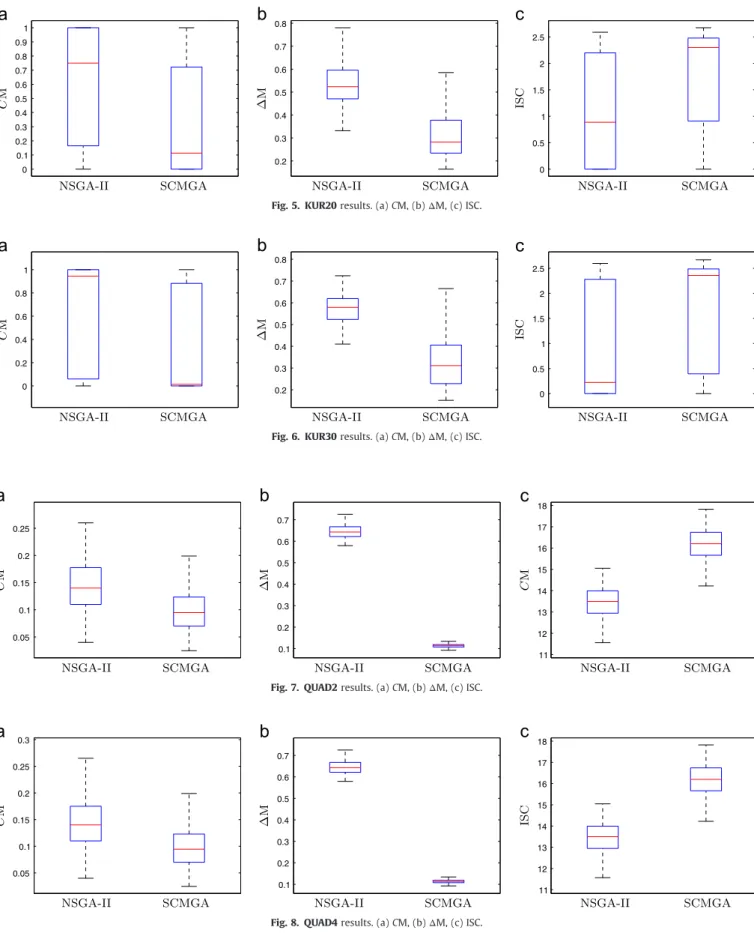
are associated to better spaced Pareto-fronts.Fig. 5. KUR20results. (a)CM, (b)ΔM, (c) ISC.
Fig. 6. KUR30results. (a)CM, (b)ΔM, (c) ISC.
Fig. 7. QUAD2results. (a)CM, (b)ΔM, (c) ISC.
Integrated sphere counting(ISC): The integrated sphere counting is used to estimate the quality of the approximated Pareto-sets achieved by the algorithms under analysis. The procedure for ISC
calculation is presented in Algorithm 6. In this algorithm, the
symbolnris the number of radii for which the sphere counting is
applied and rd is the vector of radii to be evaluated. In all
executions here, the values nr¼11 and rd¼ ½0:01;…;0:1 were adopted. Notice that, when comparing Pareto-estimates coming from two algorithms, the ISC metric is applied only to the points of
an algorithm that are non-dominated with regard to the points obtained by the other algorithm. In this way, the only relevant feature to be measured is the spread of solutions in the Pareto-estimate set. The ISC metric measures the sample effectiveness of each Pareto-set estimate under different sampling distances. The more regular is the distribution of samples, and the more
fine-grained is the sampling, the ISC metric will be greater. In
this sense, the ISC assigns higher values to better Pareto approximations.
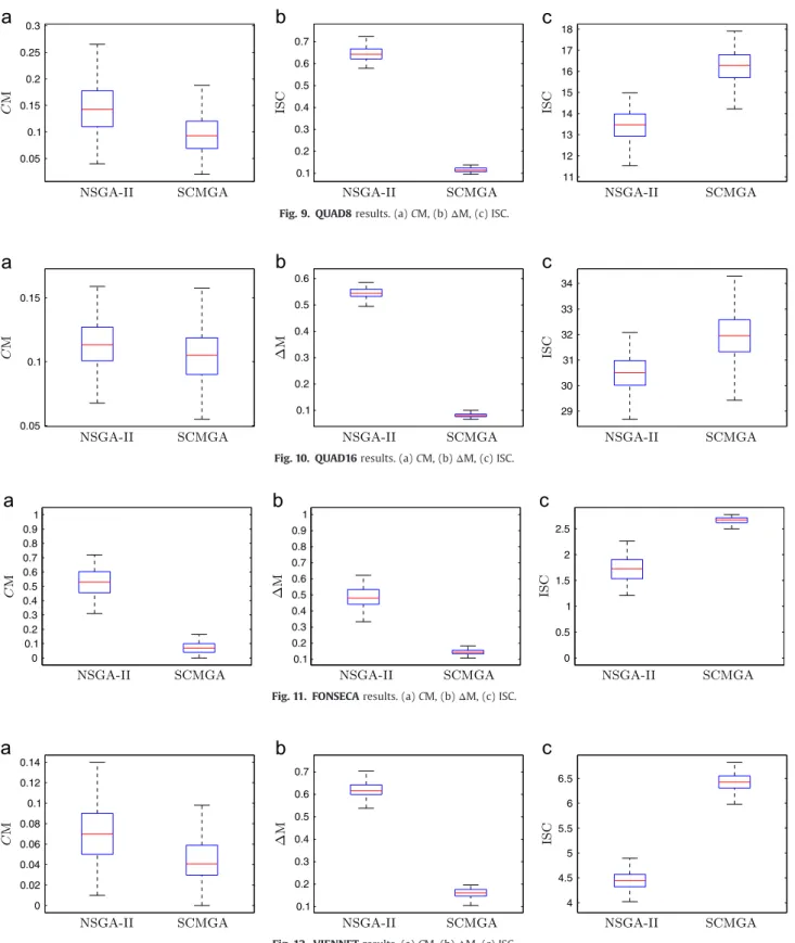
Fig. 9. QUAD8results. (a)CM, (b)ΔM, (c) ISC.
Fig. 10. QUAD16results. (a)CM, (b)ΔM, (c) ISC.
Fig. 11. FONSECAresults. (a)CM, (b)ΔM, (c) ISC.
Algorithm 6. Pseudocode for the ISC algorithm.
1: procedureISC (A,nr,rd)
2: ISC’0
3: fori¼1 tonrdo
4: C’A
5: ci’1
6: r’rdðiÞ
7: Place a sphere of radiusrcentered at any point ofC
8: whilejCj40do
9: LetRdenote the points ofCinside that sphere
10: C’C R
11: Among the remaining points, center the sphere at
the point which is closest to the previous center;
12: ci’ciþ1
13: end while
14: ISC’ISCþci
15: end for
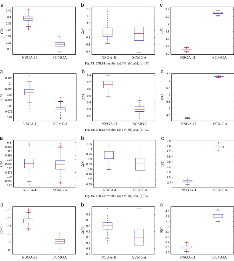
16: end procedure Fig. 13. DTLZ1results. (a)CM, (b)ΔM, (c) ISC.
Fig. 14. DTLZ2results. (a)CM, (b)ΔM, (c) ISC.
Fig. 15. DTLZ3results. (a)CM, (b)ΔM, (c) ISC.
These quality metrics have been chosen due to their efficiency and low computational complexity. Note that the comparison procedure described earlier in this section can be used with any
of these three metrics. However, in the specific case of
Δ
M, thesteps 3a–3c of the performance comparison procedure should not
be executed, since this metric requires that the input sets have the same number of elements. Besides, the permutation tests are not necessary for this metric, since it does not require pairwise comparisons.
The comparison of the algorithms has been performed using
stochastic dominance, as shown in Eq.(7). A visual information of
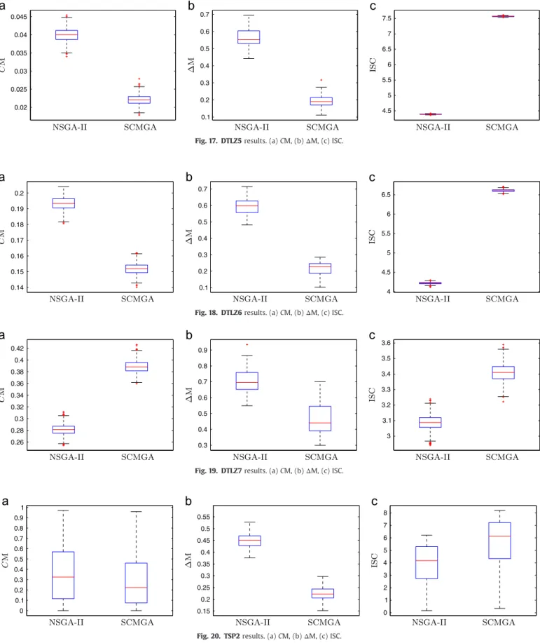
Fig. 17. DTLZ5results. (a)CM, (b)ΔM, (c) ISC.
Fig. 18. DTLZ6results. (a)CM, (b)ΔM, (c) ISC.
Fig. 19. DTLZ7results. (a)CM, (b)ΔM, (c) ISC.
this comparison is provided using box plots, in which the hor-izontal lines represent (from bottom to top): quantile 0.025, quantile 0.25, quantile 0.50, quantile 0.75 and quantile 0.975.
5.2. Numerical results
This section presents the results achieved by the NSGA-II and the SCMGA algorithms in the benchmark problems that are stated in the Appendix. The comparison of the results has been per-formed using the stochastic dominance procedure. Finally, the results of the comparisons are illustrated using box plots.
Both algorithms have been set using the same parameters:
Population size: 100 individuals.
Stop criterion–maximum number of function evaluations:
○ QUAD2: 10,000 evaluations.
○ KUR10andQUAD4: 20,000 evaluations.
○ FONSECA,VIENNET,DTLZ1,DTLZ2,DTLZ3,DTLZ4,DTLZ5,
DTLZ6andDTLZ7: 30,000 evaluations. ○ KUR20: 35,000 evaluations.
○ QUAD8: 40,000 evaluations. ○ KUR30: 50,000 evaluations.
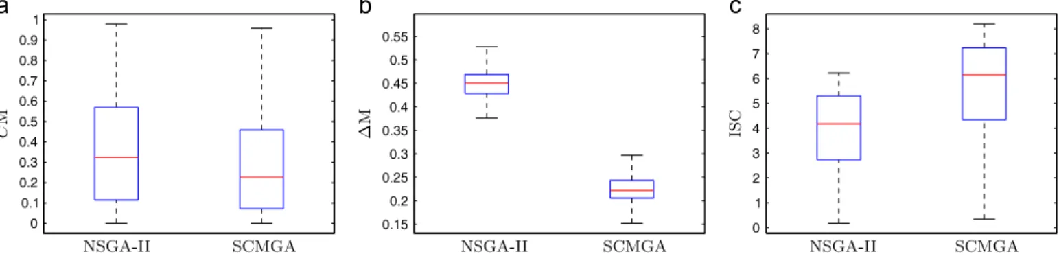
○ TSP2: 75,000 evaluations.
○ QUAD16: 80,000 evaluations.
○ TSP3: 100,000 evaluations.
Crossover probability (per pair): 0.90.
Crossover
η: 20.
Mutation probability (per individual): 1=n.
Mutation
η: 20.
Maximum archive size:
○ QUAD2andTSP2: 50 individuals.
○ KUR10,KUR20,KUR30,QUAD4,FONSECA,VIENNET,TSP3,
DTLZ1, DTLZ2, DTLZ3, DTLZ4, DTLZ5,DTLZ6 and DTLZ7: 100 individuals.
○ QUAD8: 200 individuals. ○ QUAD16: 400 individuals.
Number of algorithm runs: 100 (per instance).
Number of permutation tests: 1000 (per instance).
The
Δ
metric (9)depends on the extreme points of the realPareto-fronts. The exact extreme points have been used in the QUAD, KUR, FONSECA, VIENNET and DTLZ to evaluate such a metric, since these points are known from the literature. On the other hand, the exact mono-objective optima are not known for the TSP instances, since they have been generated at random. In order to surpass such a limitation, the best solution achieved for each objective, considering all algorithm runs, has been adopted as the respective extreme point.
Figs. 4–6show the results observed for the instances KUR10,
KUR20 and KUR30 respectively. Figs. 7–10 show the results
observed for the instancesQUAD2,QUAD4,QUAD8andQUAD16.
Fig. 11shows the result which has been observed for the instance
FONSECA, andFig. 12shows the result which has been observed
for the instanceVIENNET.Figs. 13–19show the results observed
for the seven DTLZ instances. Finally,Figs. 20 and 21show the
results observed for the instancesTSP2andTSP3.
From the box plots, it is easy to note that the SCMGA stochastically dominates the NSGA-II algorithm in most part of cases for all performance metrics (the quantiles of the SCMGA are better than the corresponding quantiles of the NSGA-II). The only exception is the coverage metric (CM) for the instance DTLZ7, in which NSGA-II achieved better results. However, it should be noticed that the proposed algorithm outperformed the original
NSGA-II for both,
Δ
M andISC, in the DTLZ7 instance. The analysisof the instances of KUR problem suggest that the SCMGA is less affected by the increase in the problem dimension than the NSGA-II, since the difference between the two algorithms increases with the problem dimension. In all instances of problem QUAD, the Fig. 21. TSP3results. (a)CM, (b)ΔM, (c) ISC.
Table 1
Processing time per run (in p.u.).xis the mean computation time andsis the standard deviation of computation time in 100 algorithm runs.
Instance NSGA-II SCMGA Base(s)
x=base s=base x=base s=base
KUR10 1.00 0.01 1.06 0.02 11.90
KUR20 1.00 0.01 1.06 0.01 19.95
KUR30 1.00 0.01 1.06 0.00 28.06
QUAD2 1.06 0.08 1.00 0.05 43.51
QUAD4 1.00 0.05 1.01 0.08 54.44
QUAD8 1.00 0.05 1.00 0.04 91.56
QUAD16 1.11 0.01 1.00 0.01 287.65
FONSECA 1.00 0.12 1.07 0.16 36.56
VIENNET 1.00 0.00 1.00 0.00 17.72
DTLZ1 1.00 0.02 1.06 0.01 18.83
DTLZ2 1.00 0.01 1.03 0.00 18.45
DTLZ3 1.00 0.01 1.07 0.01 18.99
DTLZ4 1.00 0.00 1.03 0.00 18.42
DTLZ5 1.00 0.01 1.03 0.00 18.55
DTLZ6 1.00 0.00 1.03 0.00 18.41
DTLZ7 1.00 0.00 1.04 0.00 18.16
TSP2 1.01 0.01 1.00 0.03 56.53
TSP3 1.00 0.01 1.03 0.02 68.37
decision variable space has dimension 20, and the dimension of the objective space varies. The results are similar in all cases, what suggests that the number of objectives does not affect the relative efficiency between the algorithms. In a wide analysis, it is possible to see that the proposed algorithm can obtain a bigger amount of
efficient solutions than the NSGA-II. Besides, the solutions
achieved by the SCMGA are often better spaced into the objective domain, what is also highly desirable.
The computation times required by both algorithms are shown inTable 1. The simulations have been performed on a single core of an iMac 27 (model 2011), with Core i7 3.4 GHz processor and 16 GB RAM, using Matlab 2010. In this table, it is shown the mean and the standard deviation observed amongst the runs, in p.u. values. It is possible to note that the difference between the
algorithm processing times is not significant in any of the
instances considered. In the worst case, the proposed algorithm is less than 10% slower than the original NSGA-II and it is faster in some instances. It means that the overhead caused by the
employ-ment of the self-controlled operators is not significant when
compared to the other operations required by the algorithm. The reader should notice that such a difference would be even smaller in problems in which the time required to evaluate the function is high, such as several real-world problems as the application example presented next in this paper.
6. Application study: polymer extrusion process
This section presents a brief explanation about the polymer extrusion process, which constitutes the system to which the proposed methodology is applied.
Single screw extrusion is one of the most important polymer processing technologies, allowing the production of products such as pipes,film, profiles, andfibers. Basically this process consists in feeding a solid polymer at the beginning of the system (in the hopper), melting and homogenizing it and forcing the melted
polymer to pass through a tool called the die that gives thefinal
shape to the product to be obtained. Fig. 22 illustrates this
procedure. The extruder is constituted by: (i) a hopper, where the solid polymer with the shape of pellets is fed; (ii) a heated barrel; (iii) an Archimedes-type screw rotating inside the barrel at
a given speed (N); (iv) heater bands, with temperature defined by
the operator and (v) a die.
The process performance depends on three different type of parameters: the polymer properties, the system geometry and the operating conditions. The different polymers are characterized by
properties such as thermal (e.g., heat conduction coefficient,
melting temperature and heat capacity), physical (e.g., friction
coefficients and density) and rheological (which is a measure of
the resistance of the polymer to theflow). Usually, the process is
optimized in order to process a single polymer, thus the properties are, in this case, constant. In the most simple case, a conventional
screw with three geometrical zones, as the one shown inFig. 22,
Fig. 23.Thermo-mechanical functional process steps.
Table 2
Optimization runs.
Case Optimization type Decision variables Objectives
1 Operating conditions N,Tb1,Tb2,Tb3 Q,Lmelt
2 Operating conditions N,Tb1,Tb2,Tb3 Q,Tmelt
3 Operating conditions N,Tb1,Tb2,Tb3 Q,WATS
4 Operating conditions N,Tb1,Tb2,Tb3 All
5 Screw geometry L1,L2,H1,H3,P,e Q,Power
6 Screw geometry L1,L2,H1,H3,P,e Q,WATS
7 Screw geometry L1,L2,H1,H3,P,e All
8 Both N,Tb1,Tb2,Tb3 Q,Power
9 Both N,Tb1,Tb2,Tb3 Q,WATS
10 Both N,Tb1,Tb2,Tb3 All
Table 3
Objectives, aim of optimization and range of variation.
Objective Aim of optimization Range of variation
Output (kg/h) Maximization [1, 20]
Length for melting (m) Minimization [0.2, 0.9]
Melt temperature (1C) Minimization [150, 210]
Power consumption (W) Minimization [0, 9200]
is used. First, appears a screw section with constant depth (H1), the feed section. Then, there is a compression section where the depth
varies betweenH1andH3. Finally, there is a metering section with
a constant but smaller depth (H3). The screw is also characterized
by the pitch (P) and theflight width (e). The operating conditions
are the variables that are controlled by the operator of the machine. In the present case these variables are the screw rotation
speed (N) and the barrel temperature profile (Tb1,Tb2andTb3).
The main functions of the extruder are to transport the solid material from the hopper to the heated barrel zone, to melt the polymer, to homogenize and mix the melted polymer with the additives usually present and to create the necessary pressure which enables the polymer to pass through the die at the desired output. As stated above, the performance of the extruder depends on the polymer properties, system geometry and operating con-ditions. Taking this into account a thermo-mechanical environ-ment is developed in which the polymer passes through different thermal and physical states (seeFig. 23): (i)first, the solids are fed into the hopper where, by action of gravity, they are transported inside the barrel (solids conveying in the hopper); (ii) then, by
action of the screw rotation and due to the friction between the screw and barrel walls the solid polymer is pressurized and a solid bed is formed and, simultaneously, the polymer is transported to the heated barrel zone (solids conveying in the screw); (iii) at this point, due the heat generated by friction and the heat conducted
from the barrel a melt film is formed (delay zone); (iv) then, a
specific melting mechanism develops, characterized by the
exis-tence of a melt pool and meltfilms around the solid bed (melting
zone); (v)finally, the polymer is pressurized and is transported to
the die (conveying zone).
The modeling of this process involves the linkage of all those functional zones using the appropriate boundary conditions. The
program developed is based onfinite differences, were central and
backward differences are applied for thefirst order derivatives and
the implicit Crank–Nicolson scheme is applied for the second
order derivatives. The system of equations resulting from the analysis, momentum and energy equations, was solved using the method of Gauss elimination with pivoting. The stability of the solutions was assured taking into account the convergence of
the velocityfield developed, simultaneously with the convergence
1.5 1.55 1.6 1.65 1.7 1.75 1.8 1.85 1.9 Output,kg/hr
Length,m
RPSGA
[0.8, 1.0] [0.6, 0.8) [0.4, 0.6) [0.2, 0.4) [0.0, 0.2)
1.5 1.55 1.6 1.65 1.7 1.75 1.8 1.85 1.9 Output,kg/hr
Length,m
NSGA−II
1.5 1.55 1.6 1.65 1.7 1.75 1.8 1.85 1.9 Output,kg/hr
Length,m
NSGA−II
[0.8, 1.0] [0.6, 0.8) [0.4, 0.6) [0.2, 0.4) [0.0, 0.2)
1.5 1.55 1.6 1.65 1.7 1.75 1.8 1.85 1.9 Output,kg/hr
0.125 0.13 0.135 0.14 0.125 0.13 0.135 0.14
0.125 0.13 0.135 0.14 0.125 0.13 0.135 0.14
Length,m
SCMGA
in temperature. More details of the modeling routine
implemen-ted can be found elsewhere (Gaspar-Cunha, 2009). Also, due to the
complexity of the process, in each functional zone (as identified in
Fig. 23) the existence of multiple zones is considered and solved simultaneously, i.e., the convergence must be assured simulta-neously for the different zones.
The program developed is able to compute some important performance characteristics of the process as a function of the polymer properties, system geometry and operating conditions. The process performance is characterized by the mass output of
the machine (Q), the average melt temperature of the polymer at die exit (Tmelt), the power consumption required to rotate the screw (Power), the capacity of pressure generation (Pmax), the mixing capacity measure by the average of deformation (WATS) and the length of screw required to melt the polymer (Lmelt). Those
are the objectives that are employed in the definition of the
multiobjective optimization problem studied here.
The interested reader mayfind further information about the
simulation of polymer extrusion processes in such asVergnes et al.
(1998)andCassagnau et al. (2007). The topic of optimization of
0 4 8 12 16 20
0.1 0.3
Q (kg/hr)
0 4 8 12 16 20
0.1 0.3
Q (kg/hr)
0 4 8 12 16 20
150 170 190 210 230
Q (kg/hr)
Tmelt (ºC)
RPSGA NSGA−II
0 4 8 12 16 20
150 170 190 210 230
Q (kg/hr)
Tmelt (ºC)
RPSGA SCMGA
0 4 8 12 16 20
0 250 500 750 1000
Q (kg/hr)
WATS
RPSGA NSGA−II
0 4 8 12 16 20
0 250 500 750 1000
Q (kg/hr)
WATS
RPSGA SCMGA
polymer extrusion processes has been also studied in several
works, for instance Smith et al. (1998),Sienz et al. (2006), and
Lebaal et al. (2009). It is also worthy to mention that, as the simulation of the polymer extrusion process is computationally expensive, the usage of meta-models (or surrogate models) may be useful for reducing the number of calls of the system numerical model. Some examples of usage of such models may be found, for
instance, in Wanner et al. (2008) which presents a local
meta-modeling approach, and in Giri et al. (2013) which presents a
global approach.
7. Results: application to polymer extrusion
In this section, the proposed algorithm is employed for the study of variable setup in a polymer extrusion system. In the study conducted here, three algorithms are compared: the basic NSGA-II,
the proposed SCMGA, and the RPSGA (Gaspar-Cunha and Covas,
2004; Gaspar-Cunha, 2009). This last algorithm is also used here because it was employed, in former studies, for the multiobjective optimization of the same polymer extrusion system studied here, and therefore it provides some reference for the evaluation of the behavior of other algorithms in this problem. All the tests reported
in this section were performed with a fixed budget of 20,000
function evaluations for each algorithm.
Three different types of studies were carried out as shown in
Table 2. First, only the operating conditions (i.e.,N,Tb1,Tb2, and
Tb3) were considered as decision variables – in cases 1–4. In a
second set of studies, the aim was to optimize the screw geometry (i.e.,L1,L2,H1,H3,P, ande)–in cases 5–7. Finally, both types of
decision variables were considered–in the cases 8–10. Due to the
complexity of the process and with the aim of understanding
better the variable interactions in the optimization procedure, in some preliminary studies only two objectives were considered in each run. In this case the mass output was considered the most
important objective, in order to increase the profits, being used in
all optimization runs.Table 3lists the objectives used, the aim of
optimization and their range of variation.
A statistical method based on attainment functions was applied
to compare thefinal population for all runs. The method attributes
to each objective vectorza probability that this pointzis attained in one single run. It is not possible to compute the true attainment function, but it can be estimated based on an approximation to set samples, i.e., different approximations obtained in different runs,
denoted as empirical attainment function (EAF) (Fonseca and
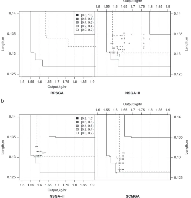
Fleming, 1996). The differences between two algorithms can be visualized by plotting the points in the objective space where the differences between the empirical attainment functions of the two algorithms are significant (López-Ibánez et al., 2010).
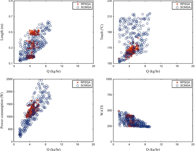
Fig. 24shows a comparison for case 1 between NSGA-II, RPSGA and SCMGA. Ten different runs for case 1 were performed. For this particular case, NSGA-II is slightly better than RPSGA, but SCMGA is better than the NSGA-II, since there are some black dots that indicate that the SCMGA is better in at least 80% of the runs than
NSGA-II. Figs. 25–27 show the results obtained by the different
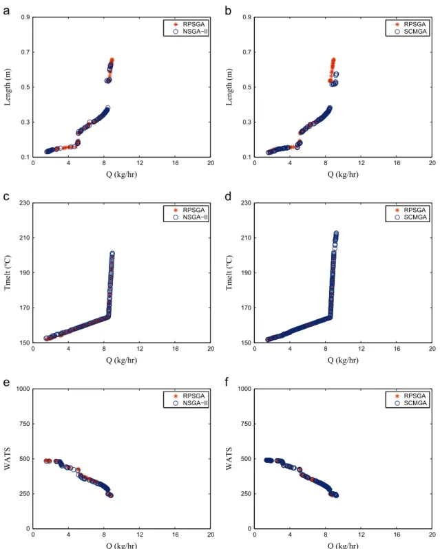
methods (RPSGA, NSGA-II and SCMGA) for the remaining cases
studied. Fig. 25 shows that for the cases were the operating
conditions were optimized the better performance of the SCMGA is mainly accomplished in the extreme limits of the objective
functions. In case study 4, in which all five objectives are
considered, the SCMGA was able tofind Pareto-optimal solutions
much more spread over the search space. The results for cases 7 and 10 are very similar to results obtained for case 4. Finally,
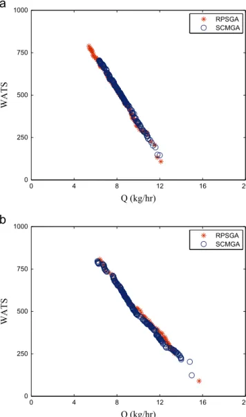
Fig. 27shows the results for cases 6 and 9 were both objectives are
0 4 8 12 16 20
0.1 0.3 0.5 0.7 0.9
Q (kg/hr)
Length (m)
RPSGA SCMGA
0 4 8 12 16 20
150 170 190 210 230
Q (kg/hr)
Tmelt (ºC)
RPSGA SCMGA
0 4 8 12 16 20
0 500 1000 1500 2000 2500
Q (kg/hr)
Power consumption (W)
RPSGA SCMGA
0 4 8 12 16 20
0 250 500 750 1000
Q (kg/hr)
WATS
RPSGA SCMGA
to be maximized. In these cases the differences between the two methods considered were not so evident due to the fact that now, in the extrusion process, the geometry of the system is allowed to vary. The effect of geometry variation is evident if these results
were compared with the results of case 3 represented inFig. 25(e)
and (f).
The outcomes of the multiobjective optimization–the
Pareto-optimal solutions–may be used by a decision-maker as a means
to assist the choice of the parameter configuration to be employed
in the manufacturing of a specific product. The Pareto-optimal set
carries the information about the limits of performance of the plant for that task, including the information about the trade-offs involved in the choice between different Pareto-optimal solutions.
In this specific case study, the trade-offs are related to energy
consumption, production capacity and product quality. A good description of the Pareto-set covering all its extension with a uniform sampling is important in order to provide the full set of alternatives to the decision-maker. The SCMGA method was
shown to be an effective way to find out good descriptions of
the Pareto-set that were not possible to obtain by other algo-rithms, mainly when more than two objectives are considered. This suggests that the proposed methodology is suitable for dealing with problems in application domains similar to the one studied here.
The archive reduction plus the space-filling crossover were
included in the canonical NSGA-II, with the hybrid algorithm (the SCMGA) used for the purpose of performing some comparisons with the original algorithm. In this way, some quantitative
comparisons were performed, showing a significant
enhance-ment of the resulting Pareto-set descriptions obtained by the hybrid algorithm, in several benchmark problems. The numerical experiments that have been conducted on those benchmark functions also showed that the computational overhead caused by the proposed operators is smaller than 10%, not considering
the computational effort devoted to objective function
evaluation.
The proposed SCMGA was employed in the multiobjective
optimization of a polymer extrusion system. Some specific
con-clusions about the case study are: (i) The SCMGA was able to generate a much enhanced description of the Pareto-set of the problem, providing both a more uniform sampling and a more complete description of the whole extension of that set. (ii) It was
also verified that the difference of the performance of SCMGA in
comparison with the other algorithms was greater in the case of three objectives than in the case of two objectives.
Those features indicate that the proposed SCMGA may be a good choice as a tool for providing the detailed information about the Pareto-optimal set, in order to assist the decision-maker in
tasks such as the choice of the configuration of a polymer
extrusion machine.
Acknowledgments
This work was supported by the Brazilian agencies CNPq, CAPES and FAPEMIG. The authors also acknowledge the support by a Marie Curie International Research Staff Exchange Scheme Fellowship within the 7th European Community Framework Programme.
Appendix A. Description of benchmark problems
The benchmark multiobjective optimization problems employed in the numerical tests are described in this appendix.
Kursawe problem (Kursawe, 1991):
Xn
¼arg min
X
f1¼n∑1
i¼1
10exp 0:2
ffiffiffiffiffiffiffiffiffiffiffiffiffiffiffiffiffiffiffiffiffiffiffiffi x2
i þx2iþ1
q
h i
f2¼ ∑ n
i¼1½j
x0:8
i jþ5 sinðx3iÞ
8 > > > > <
> > > > :
ð10Þ
subject to 5rxir5 8i¼1;…;n ð11Þ
in whichnis the number of problem variables.
Three instances of the Kursawe problem are considered here:
KUR10:n¼10; KUR20:n¼20; KUR30:n¼30.0 4 8 12 16 20
0 250
Q (kg/hr)
0 4 8 12 16 20
0 250 500 750 1000
Q (kg/hr)
WATS
RPSGA SCMGA