Abstract
In this paper, we present a new numerical method for nonlinear vibrational analysis of Euler-Bernoulli beams. Our approach is based on the continuous Galerkin-Petrov time discretization meth-od. The Euler-Bernoulli beam equation which governs its vibrations is transformed into set of ordinary differential equations and the presented method is employed in order to investigate the vibration-al response. A comparison is made between present method and different other methods available in literature. It is observed that the obtained results are in strong agreement with other results in literature. We conclude that the present method has a great poten-tial to deal with nonlinear vibration analysis problems of beams and related structures like rods and shafts.
Keywords
Nonlinear vibration; Euler-Bernoulli beams; Time discretization; Numerical method
Nonlinear Vibration Analysis of Euler-Bernoulli Beams by Using
Continuous Galerkin-Petrov Time-Discretization Method
1 INTRODUCTION
In the design and fabrication of many engineering structures and machines, vibrational analysis and dynamical response of structures like beams (or rods or shafts) are important factor to investigate in order to increase the performance of these structures. For the analysis of complex engineering struc-tures like bridges, tall buildings, vehicle guide-ways, huge cranes, turbines and compressor blades, beams can be used as simple model. The dynamical response of beams is governed by linear as well as nonlinear differential equations both in space and time. To study their behavior it is therefore important to design methods for the numerical solutions of these partial differential equations. In this respect, recently some approximate analytical techniques (see for instance, Barari et al., 2010; Bayat et al., 2010; Baghari et al., 2014; Jafari et al., 2014; Bayat et al., 2011;, Ganji, 2012; He, 1999; He, 2006; Khan et al., 2012; Liu and Gurram, 2009; Mirgolbabaei et al., 2010; Sfahani et al., 2011) as well as numerical methods by Lai et al. (2008) (see also, Boukhalfa et al., 2010; Da Silva
M. Sabeel Khan a, * H. Kaneez a
a Department of Applied Mathematics,
Institute of Space Technology, 44000 Islamabad, Pakistan
http://dx.doi.org/10.1590/1679-78253327
et al., 2009; Ganji et al., 2011) and references therein, have been proposed to investigate the nonlin-ear vibrations of beams for designing and fabrication purpose.
The theory of Euler-Bernoulli beams which is based on the assumption that beam curvature is related to its bending moment provides a good explanation of long isotropic bar’s bending behavior. Several methods have been proposed for obtaining solution to the nonlinear equations of motions governing the Euler-Bernoulli beam’s response. Nonlinear vibrations of the Euler-Bernoulli beam has been investigated by Barari et al. (2011) using the Variational iteration and parameterized per-turbation methods. Nikkar et al. (2014) studied the nonlinear vibration response of Euler-Bernoulli beam by approximate analytical techniques where they utilized Variational He’s approach and La-place iteration technique in order to solve the respective nonlinear governing equations. Pakar and Bayat (2013) applied a max-min approach, also by He, to investigate the nonlinear vibrational re-sponse of Euler-Bernoulli beams subjected to an axial load. Nonlinear behavior of Euler-Bernoulli beam with different end conditions has also been studied by Rafieipour et al. (2014) using Laplace iteration method. Lindstedt-Poincare techniques for non linear vibrational analysis have been em-ployed to double-clamped and simply-supported beams subjected to an axial load by Ahmadian et al. (2009). Javanmard et al. (2013) used He’s Energy method in order to get solution of nonlinear vibration problem of Euler-Bernoulli beam subjected to axial loads. A similar study has been per-formed earlier by Pirbodaghi et al. (2009) but with homotopy analysis method. The nonlinear equa-tion of moequa-tion for large amplitude free vibraequa-tional analysis of Euler-Bernoulli beam resting on vari-able elastic foundation was solved by Mirzabeigy and Madoliat (2016) with the application of sec-ond order homotopy perturbation method. Moreover, the nonlinear vibrational response of Euler-Bernoulli beams with geometric nonlinarity and subjected to axial loads was computed by Johnson et al. S. (2014) where they used a differential transform and two auxiliary parameter based ho-motopy analysis techniques.
Here, in this article, we present a new approach to solve equations of motions governing the dy-namics of Euler-Bernoulli clamped-clamped-beam which is fixed from one end. This article is orga-nized as follows. In Section II, a mathematical framework governing the nonlinear vibrations of Eu-ler-Bernolulli beam is presented. In Section III, continuous Galerkin-Petrov time-discretization method is developed. In Section IV, the developed method afterwards applied to the governing equations of Euler-Bernoulli beam presented in Section II. In Section V, simulations data and nu-merical results are discussed. In last Section, conclusions are drawn based on the obtained simula-tion results in Secsimula-tion V.
2 MATHEMATICAL FORMULATION
,
2
0 2 2 2 2 2 2 2 4 4t)
q(x,
dx
x
Y
x
Y
L
EA
KY
t
Y
d
x
Y
F
t
Y
x
Y
EI
L
(1)where,
d
is the coefficient of viscous damping,K
is the stiffness of foundation and q(x,t) is thetransverse directional load. In the absence of non-conservative forces above equation (1) reduced to
.
0
2
0 2 2 2 2 2 2 2 4 4
Ldx
x
Y
x
Y
L
EA
KY
x
Y
F
t
Y
x
Y
EI
(2)In order to undimensionalize the above equation we choose the following variables
,
~
and
~
,
~
,
~
,
~
2 44
EI
KL
K
EI
FL
F
L
EI
t
t
r
Y
Y
L
X
X
G
(3)where,
r
G is the gyration radius of the cross-section of the beam. Using equation (3) and omitting the tilde sign from the variables equations (2) thus can be written as follows.
0
2
1
1 0 2 2 2 2 2 2 2 4 4
dx
x
Y
x
Y
KY
x
Y
F
t
Y
x
Y
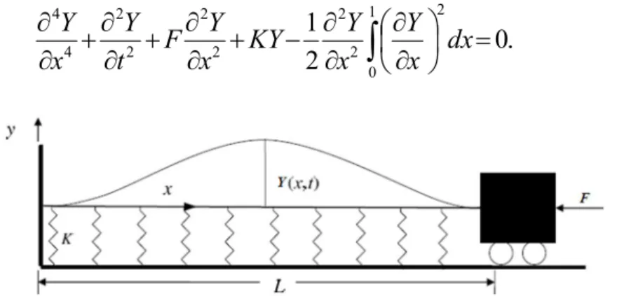
(4)Figure 1: A schematic representation of an Euler-Bernoulli beam fixed at one end and subjected to axial load.
Now, by assuming a product solution Y(x,t)
(x)
(t), where
(x) is the beam’s eigen mode,and by applying the Galerkin method, an equation governing the beam dynamics is obtained as
0
)
(
)
(
)
(
3 2 2
t
t
dt
t
d
(5)Where
and
can be determined by the relations,
1 0 2 1 0 1 0 2 1 0 ) (
dx
dx
F
dx
dx
K
iv
and.
Moreover, in order to complete the above problem description, the beam is subjected to follow-ing initial conditions
, 0 ) 0 ( , ) 0
(
dt d
A
(6)where
A
is the amplitude of oscillation. Equation (5) along with initial conditions in Equation (6) governs the nonlinear vibrational response of Euler-Bernoulli beams.3 DESCRIPTION OF CONTINOUS GALERKIN-PETROV TIME-DISCRETIZATION METHOD
In this section, we present a time discretization method to solve nonlinear equations governing the dynamics of Euler-Bernoulli beams. It is easy to see that Equation (5) can be transformed into a system of nonlinear differential equations of the following form
U(t) f(t,U(t)).dt d
(7)
Where,
U
(
t
)
(
,
)
T and f denotes the vector of unknown-state variables and vector comprisingnon-linear functions in both time and space, respectively. Here,
is the first order time derivative of
.
In order to develop a numerical method to solve such dynamical systems, here, we use the concept of a Galerkin-type formulation and time-discretization. LetS
be a space of all possible solutions to set of nonlinear differential equations in Equation (7). We search a vector of unknown states U:[0,
]S such that
U(t) f(t,U(t)),t(0,
)dt
d , where
.
)
0
(
U
0U
(8)
By choosing
as a test space the problem in Equation (8) can be formulated as follows: FindS
U
such that
0 ( ) U(t)dt dtd t
VT
,
, .0
V dt t U t f t
VT With
U
(
0
)
U
0,
(9)Equation (9) is the weak form of problem in Equation (8). Now, to solve it over the time inter-val I
0, let us discretized the intervalI
into further sub-intervals with each sub-interval
n nn
t
t
I
-1,
wheren
belongs to the set
1,..., N}. Now, each interval is having the following prop-erty
nNt
nt
n1 1,
.
,
0
t
n,1t
n
t
m,1t
m
{
0
},
for
all
n
m
n,m
1,...,
N.
In order to compute the vector of state variables U(t) at time interval In, we choose
n jn,
t
Ρ
kΙ
as a set of basis functions. Here,Ρ
k
Ι
n represents the k-th degree polynomials space defined on intervalI
n by
,
:
: ;
, for all , .0
k
j
H j n j
j H
n H
n S U t Ι S U t t t Ι S
Ι u u
Ρ (10)
The vector of state variables U(t) in Equation (5) is thus approximated by
kj
n n,j
j
n
t
I
t
U
t
U
0
t
all
for
,
)
(
u
(11)Where,
u
nj are vector elements in Hilbert space SH Global vector of state variablesH
n
S
Ι
t
U
(
)
:
is in the discrete-solution spaceS
k
S
where,
C
,
:
|
,
;
for
all
1,...,
,
:
U
t
Ι
S
U
t
kΙ
S
n
N
S
k n H Ι n Hn
Ρ
with
Ι
n
Ι
n
t
n,1t
n . The symbol σ above represents a discretization parameter. The testfunc-tion V(t) is taken from discrete test space
k where,
L
,
:
|
,
;
1,...,
.
:
V
t
2Ι
nS
HV
t
Ι k-1Ι
nS
Hn
N
kn
Ρ
By denoting Vσ(t) as a discrete approximation of the test function V(t), then the weak problem in Equation (9) takes the following Variational form which states:
Find
U
t
U
o
S
k,0 such that
,
; .dt d
0 T
0
T k
V dt t U t f t V dt t U t
V
(12)Above
ok k
S
S
s
,0:
denotes the subspace of
S
k with zero as initial condition. Define a pol-ynomial
n,i
Ρ
k-1
Ι
n on the time interval I zero everywhere in the set I, except at the timeinter-val Īn = [tn–1, tn], and v∊ SH as an arbitrary scalar function then the variational problem on time interval In in Equation (12) reads
T
,
;
.
TH n.i
Ι
n,i
Ι
dt
U
t
t
dt
t
f
t
U
t
t
dt
S
d
t
n
n
v
v
v
(13)
,
.
;
.
0 j T 0 j T H i n I k n,j j n n,i I k n,j jn
t
t
dt
t
f
t
t
t
dt
S
dt
d
t
n n
v
u
v
u
v
(14)To define Basis functions in Equation (14), a mapping
M
nI
Ι
n
:
is used which maps the time intervalI
[
1
1,
]
from natural time intervalI
to physical time intervalΙ
n. Now, for everyI
t there exists
t
Ι
n such that
ˆ ;
1,...,
. 2 2 : ˆM t t -1 t t Ι n N
t n n n n
n
The basis functions defined on physical time interval
Ι
n can now be calculated in natural timeinterval as
:
1
;
0,...,
,
,j
t
jM
nt
j
k
n
:
ˆ
1
;
0,...
-
1.
.i
t
iM
nt
i
k
n
Where,
j
Ρ
k
Ι
ˆ
,
and
ˆ
i
Ρ
k-1
Ι
ˆ
are satisfying the property
1
0,j
,
ˆ
j
1
k,j
,
j
(15)k,j
Denote the Kronecker’s delta. To get a second-order approximation of discrete vector of state variablesU
(
t
)
we require to find the coefficientsu
nj;
j
0,1,2
. By using property of basis func-tion from Equafunc-tion (15) and with the applicafunc-tion of initial condifunc-tion the coefficientsu
0n can bede-termined from the following
1.
,
1
,
1 0 0
n
n
U
k n-nu
u
(16)Since, it is easy to deal with natural-time interval Î, thus Equation (14) is reconstructed into
H0
0 ˆ
n
,
2
f
M
t
ˆ
,
ˆ
jt
ˆ
ˆ
it
ˆ
d
t
ˆ
;
S
k j j n n k j T j n T j i
v
u
v
u
v
(17)where, i0,...,k-1 and
ˆ
ˆ
ˆ
.ˆ
ˆ
ˆ
:
ˆ j ,
t
t
d
t
t
d
d
i j
i
(18)
H0 0 0
T
,
wˆ
f
M
tˆ
,
ˆ
t
ˆ
ˆ
it
ˆ
l;
S
k j k l k j l j j n l n T l j n j i
v
u
v
u
v
(19)Where,
wˆ
l represents the weightst
ˆ
0
-
1
,
t
ˆ
k
1
,
and
t
ˆ
l
Ι
;ˆ
l
1
,...,
k
1
are roots of theLe-gendre polynomial Ρk-1
t . Using the abbreviation
ˆ
,
:
wˆ
ˆ
ˆ
and
:
ˆ
ˆ
.
g
:
i,,l n l l l l j.l j l
n
t
t
t
t
(20)Hence, we finally arrived at the following system of coupled equations
(
T)
n T, H
0
, ; , 0,..., -1 and ,..., ,
2
k k k
j j
i j n i,l n,l n j,i
j l f t j S i k j k
s
a b h
= = =
æ æ ö÷ö
ç ç ÷÷÷
ç ç
= çèçç çççè ÷÷÷ø÷÷÷÷ø Î = =
å
v uå
vå
u v0 0 0 (21)
with initial conditions as described in Equation (16).
3.1 Computation of Parameters
i,j,
i,j and
j,lTo compute unknown parameters in Equation (21) let us select the following set of test functions
ˆ ,
ˆ 1 4 3 ˆ ˆ , ˆˆi tj
i,j
0 tj tj
1 tj
for all i, j
0,1,2
,Where, each
ˆ
j
t
ˆ
Ρ
k
Ι
ˆ
,
ˆ
i
t
ˆ
Ρ
k-1
Ι
ˆ
,
andt
ˆ
0
-
1
,
t
1ˆ
0
,
and
t
ˆ
2
1
. By this choice of test functions
i,j,
i,j and
j,l are calculated and are given as under
,
}.
2
0,1,
,
all
for
,
4
1
,
3
,
,
0
,
4
1
,
0
,
,
,
1
,
2
1
, 1 , 1 2 , 1 0 , 1 0 , 0 1 , 1 0 , 0 2 , 0 1 , 0 0 , 0 1 , 1 1 , 0 0 , 1 0 , 0 2 , 0 2 , 1 1 , 0 0 , 0
j
i
i,j j i
4 APPLICATION TO GOVERNING EQUATIONS OF EULER-BERNOULLI BEAMS
The method presented in Section 3 is applied to motion equation in Equation (5) and the obtained discrete set of equations are solved using numerical algorithm outlined as under
Numerical Algorithm:
Step 1: Initialize the known parameters
and
Step 3: Set the initial conditions at time
t
nas0
,
11
m
n m
n
A
Step 4: First solve the following equations for unknowns nm m n
,
1 1 1 3 1 3
1 1 1 1 1 1
8
2
1
2
1
2
8
1
2
1
m n m n m n m n n m n m n m n m n m n n m n m n m n
Step 5: Using the computed values for
nm and m n
from Step 4, Solve the following nonlinear equations for 1and
nm1.
m
n
4
4
6
4
6
3 1 3 3 1 1 1 1 1 1 1 1 1
m n m n m n m n m n m n n m n m n m n m n m n n m n m n
Step 6: Use the computed values of
nm1 and1
m n
from Step 5 to get the numerical values of
nmand
nm from Step 4 by back substitution.Step 7: Compute the solution at time step
t
n by equation (11)Step 8: Update the solution for the next time iteration by
.
,
1 11 1 1
1
nm m n m n mn
Step 9: Update the time step
t
n
t
n
nStep 10: Go to Step 4.
5 RESULTS AND DISCUSSIONS
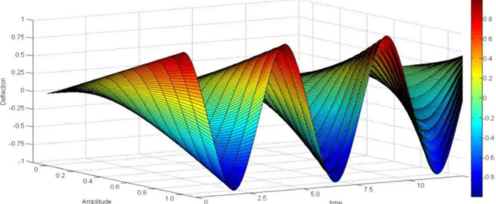
Figure 2: Non-dimensional deflection with varying values of amplitude
A
and with parametric values
1
.
0
.
In Table 1 and Table 2, a comparison is made between the presented method and four different methods, with semi-analytical approach by Barari et al. (2011), with a semi-analytical method by Nikkar et al. (2014), with semi-analytical approach by Johnson et al. (2014) and with numerical method RK-4. It is seen that the computed values of deflection at the center of the beam for differ-ent values of maximum amplitude of oscillation are in strong agreemdiffer-ent with the results by these methods. In Table 3, relative errors are provided which are computed by the formula
%, 100 Method
Existing by
Solution
) Method Existing
by Solution
-Method Present
by Solution
(
Wherein, Error-1 is calculated by taking RK-4 solution as an existing solution. In Error-II the existing solution is taken from the semi-analytical approach by Barari et al. (2011). Error-III is obtained by taking the existing solution form the method by Nikkar et al. (2014). In all of these calculations the errors are shown for three different amplitude of oscillation of beam over a wide range of time. From Table 3, it can be clearly seen that the results by present method converges closely to other results in literature and are in strong agreement.
A RK-4 Barari et al. (2011) Nikkar et al. (2014) Present 0.01 0.008775827082332 0.008775710513259 0.008775710509477 0.008653113482869
0.1 0.087759719142174 0.087643206097855 0.087642827100616 0.086406655501930 0.2 0.175528204796203 0.174597455961528 0.174585253116176 0.172060842262657 0.3 0.263314167649526 0.260180487515907 0.260086892907199 0.263974531478741 0.4 0.351126207698248 0.343723299721559 0.343323578255470 0.349072483074928 0.5 0.438972761263577 0.424576467617775 0.423336627126820 0.417180214867134 0.6 0.526862050755839 0.502116086386647 0.498973411668122 0.492625565690737 0.7 0.614802037962082 0.575749233260282 0.568819355464365 0.563875657455006 0.8 0.702800381522887 0.644918846456226 0.631123805468134 0.630358772839251 0.9 0.790864399137227 0.709107932868351 0.683724780583061 0.691556439573670 1.0 0.879001034896931 0.767843030699686 0.723980197798699 0.766656852847480
A
RK4
present
Barariet al.(2011)
present
Nikkar et al.(2014)
present
Johnson et al.(2014)
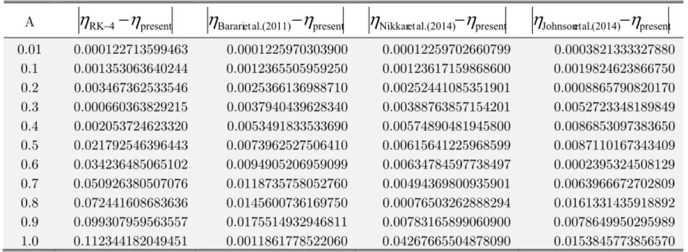
present 0.01 0.000122713599463 0.0001225970303900 0.00012259702660799 0.00038213333278800.1 0.001353063640244 0.0012365505959250 0.00123617159868600 0.0019824623866750 0.2 0.003467362533546 0.0025366136988710 0.00252441085351901 0.0008865790820170 0.3 0.000660363829215 0.0037940439628340 0.00388763857154201 0.0052723348189849 0.4 0.002053724623320 0.0053491833533690 0.00574890481945800 0.0086853097383650 0.5 0.021792546396443 0.0073962527506410 0.00615641225968599 0.0087110167343409 0.6 0.034236485065102 0.0094905206959099 0.00634784597738497 0.0002395324508129 0.7 0.050926380507076 0.0118735758052760 0.00494369800935901 0.0063966672702809 0.8 0.072441608683636 0.0145600736169750 0.00076503262888294 0.0161331435918892 0.9 0.099307959563557 0.0175514932946811 0.00783165899060900 0.0078649950295989 1.0 0.112344182049451 0.0011861778522060 0.04267665504878090 0.0153845773856570
Table 2: Differences between the time marching solution of equation (5) by presented method and different other schemes in literature. The parameters are chosen to be
1
.
0
.
A
ti-me Error-I Error-II Error-III
5 8.39406344436937 1.43006947021705 1.43006930029566 10 1.64295821637604 1.65335398475738 0.46126609193088 0.01 25 -0.40714155296337 -0.30013048066676 -0.30013048391456 50 0.34564381067195 0.70609180050204 0.70609178786218 100 0.89942811653737 1.32438720734438 1.32438716831965 5 -0.01611628030638 -2.71860640853757 -3.34003971902284 10 -2.19636228576523 0.94834463220716 -0.15087284130191 0.50 25 1.33999271743426 0.18473004818300 -0.63051410694749 50 4.46407178480245 -0.21897390156171 -1.08460097418586 100 -5.91449682727209 -0.55016306148146 -0.57899624097327 5 -5.825758083900410 0.33425814206559 -1.25501908713661 10 -0.411754581578781 -1.42949464499397 -0.67810815791013 1.00 25 -0.614810964667922 3.07084443826624 0.52366254911929 50 0.200159632081500 -0.86954946868848 0.65475889510081 100 1.993160046364360 -0.27554338389560 0.96750105622486
Table 3: Relative errors between the time marching solution of equation (5) by presented method with different other schemes in literature. The parameters are chosen to be
1
.
0
.
maximum amplitude of vibration is seen as the time marches. In Table 4, a comparison is made be-tween the accumulated errors by classical numerical scheme RK-4 and present method. Also the accu-racy of solution by both of the numerical methods is shown for two different time step sizes. In all the computations of accumulated errors in Table 4 the reference solution by Johnson et al. (2014) is taken into consideration. It is observed that our present numerical method is more accurate in predicting the solution over the classical RK-4 method. This is highly due to the fact that present method does not involve iterative time integration and therefore have less accumulated errors as shown in Table 4. Moreover, it is observed that that the accumulated error decreases with an increase in the time step size for both the classical RK-4 and present method.
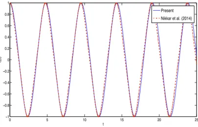
Figure 3: A comparison of time history of central deflection curve of beam. The time step used for this simulation is 0.05 and the parameters
A
1
.
0
.
Figure 4: A comparison of time history of central deflection curve of beam. The time step used for this simulation is 0.05 and the parameters
A
1
.
0
.
0 5 10 15 20 25
−1
−0.8
−0.6
−0.4
−0.2
0 0.2 0.4 0.6 0.8 1
t
η
(t
)
Present Nikkar et al. (2014)
0 5 10 15 20 25
−1
−0.8
−0.6
−0.4
−0.2
0 0.2 0.4 0.6 0.8 1
t
η
(t
)
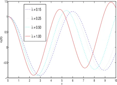
Figure 5: Time-history of central-deflection of beam with varying. The parametric value of
is chosen to be 1.0.Time - step
size
Number of time steps
Accumulated error by RK-4
Accuracy (in percent) by RK-4
Accumulated error by present method
Accuracy (in percent) by present method
5 7.1629284856E-04 7.838643342877E+01 4.7825078312E-04 8.556916328361E+01
10 4.1601192713E-04 9.991054140377E+01 2.8166615852E-04 9.996668334601E+01
25 8.9254489341E-05 9.910446043034E+01 6.3862965951E-05 9.935922760337E+01
0.05 50 1.8633928689E-04 9.809327174198E+01 1.4120960638E-04 9.855506398418E+01
100 3.6919714161E-04 9.584366665341E+01 2.9192878467E-04 9.671353538314E+01
250 7.2383261971E-04 7.572278868091E+01 5.9430126403E-04 8.006724623713E+01
500 3.7148542418E-04 9.975956260686E+01 1.8132325720E-04 1.000734824724E+02
5 5.04555298800E-05 9.82223873076E+01 2.39457037950E-05 9.91563623037E+01
10 2.64336613610E-05 1.00163169326E+02 1.36876932130E-05 1.00315112462E+02
25 4.97951263280E-05 1.00561378909E+02 2.28701839830E-05 1.01222287224E+02
0.005 50 1.70105932140E-05 9.98284057000E+01 3.19282474000E-06 9.99677923915E+01
100 3.59407763030E-05 9.96277324234E+01 6.42406862100E-06 9.99334607456E+01
250 1.61756733776E-04 9.35316240962E+01 2.41848699480E-05 9.90328882986E+01
500 4.74408476010E-05 9.94577701222E+01 1.21912724690E-05 1.00139341359E+02
Table 4: A comparison of accumulated errors and accuracy for RK-4 and present method.
0 1 2 3 4 5 6 7 8 9 10
−1 −0.5 0 0.5 1 1.5
t
η
(t)
ε = 0.15
ε = 0.25
ε = 0.50
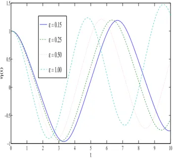
Figure 6: Time-history of central-deflection of beam with varying
. The parametric value of is chosen to be 1.0.6 CONCLUSIONS
A new numerical method is presented for nonlinear vibrational analysis of Euler-Bernoulli beams. The non-dimensional central deflection response of a clamped-clamped-Euler-Bernoulli beam (fixed from one end side) is investigated under different initial vibration amplitudes using this numerical technique. A comparison of computed results by present method is made with the results by other semi-analytical schemes in literature and the numerical values of central deflection of beam are tab-ulated. Relative errors between the present method and other semi-analytical approaches in litera-ture have been shown to observe the convergence of solution obtained by present method. Moreo-ver, a parametric study is carried out to investigate effect of different parameters on beam’s central deflection. It is worth mentioning that the obtained results by presented method are in strong agreement with results by semi-analytical approaches (for instance, Barari et al. 2011, Nikkar et al. 2014 and Johnson et al. 2014) in literature and also with classical numerical scheme RK-4. It is worthy of noting that the present scheme does not involve iterative time integration like other methods in literature and thus no associated accumulative errors. Therefore, it is capable to provide accurate results with high accuracy and convergence characteristics as can be seen by the presented results and thus can be utilized to compute dynamical response of structures like rods and shafts. We conclude that the present method has great potential in dealing with nonlinear vibrational re-sponse of beams and similar structures like rods and shafts.
Acknowledgement
The authors are grateful to the anonymous reviewers for their careful reading and constructive sug-gestions in order to improve the quality of this research article.
0 1 2 3 4 5 6 7 8 9 10
−1
−0.5 0 0.5 1 1.5
t
η
(t
)
λ = 0.15
λ = 0.25
λ = 0.50
References
Ahmadian, M.T., Mojahedi, M., Moeenfard, H. (2009). Free vibration analysis of a nonlinear beam using homotopy and modified Lindstedt-Poincare Methods. Journal of Solid Mechanics. 29-36.
Bagheri, S., Nikkar, A., Ghaffarzadeh, H. (2014). Study of nonlinear vibration of Euler-Bernoulli beams by using analytical approximate techniques. Lat. Am. J. Solids Struct. 11: 157-168.
Barari, A., Ganjavi, B., Ghanbari, J M., Domairry, G. (2010). Assessment of two analytical methods in solving the linear and nonlinear elastic beam deformation problems. Journal of Engineering, Design and Technology, 8(2):127– 145.
Barari, A., Kaliji, H.D., Ghadimi, M., Domairry, G. (2011). Non-linear vibration of Euler-Bernoulli beams. Lat. Am. J. Solids Struct. 8: 139-148.
Barari, B., Kimiaeifar, A., Domairry, G., Moghimi, M. (2010). Analytical evaluation of beam deformation problem using approximate methods. Songklanakarin Journal of Science and Technology, 32(3):207–326.
Bayat, M., Pakar, I., Bayat, M., (2011). Analytical study on the vibration frequencies of tapered beams, Lat. Am. J. Solids Struct. 8(2):149-162.
Bayat, M., Shahidi, M., Barari, A., Domairry, G. (2010). On the approximate analysis of nonlinear behavior of struc-ture under harmonic loading. International Journal of Physical Sciences, 5(7):1074–1080.
Boukhalfa, A., Hadjoui, A., (2010). Free vibration analysis of an embarked rotating composite shaft using the hp-version of the FEM, Lat. Am. J. Solids Struct. 7:105–141.
Da Silva, J. C. R. Á., Beck, A. T., da Rosa, E., (2009). Solution of the stochastic beam bending problem by Galerkin method and the Askey-Wiener scheme, Lat. Am. J. Solids Struct. 6(1):51-72.
Ganji, D. D. (2012). A semi-Analytical technique for non-linear settling particle equation of Motion, Journal of Hy-dro-environment Research 6(4): 323-327.
Ganji, S.S., Barari, B., Ganji, D.D., (2011). Approximate analyses of two mass-spring systems and buckling of a column. Computers & Mathematics with Applications, 61(4):1088–1095.
He, J. H. (2006). Some asymptotic methods for strongly nonlinear equations, International Journal of Modern Phys-ics B 20(10):1141-1199.
He., J.H. (1999). Variational iteration method – a kind of non-linear analytical technique: Some examples. Interna-tional Journal of Nonlinear Mechanics, 34:699–708.
Jafari, S.S., Rashidi, M.M., Johnson, S. (2014). Analytical solution of the nonlinear vibration of euler-bernoulli beams via the homotopy analysis method and differential transform method. Int. J. of Appl. Math and Mech.10 (9): 96-110.
Javanmard, M., Bayat, M., Ardakani, A. (2013). Nonlinear vibration of Euler-Bernoulli beams resting on linear elastic foundation. Steel Comp. Struct. 15(4):
Jian-She Peng, J., Yan Liu, Y., Yang, J. (2010). A semi-analytical method for nonlinear vibration of Euler-Bernoulli beams with general boundary conditions. Math. Probl. Eng.
Khan, Y., Taghipour, R., Fallahian, M., Nikkar, A., (2012). A new approach to modified regularized long wave equa-tion, Neural Computing and Applications doi:10.1007/s00521-012-1077-0
Lai, H.Y., Hsu, J.C., Chen, C.K., (2008). An innovative eigenvalue problem solver for free vibration of Euler-Bernoulli beam by using the Adomian Decomposition Method, Computers and Mathematics with Applications, 56: 3204-3220.
Liu, Y., Gurram, C. S., (2009). The use of He’s Variational iteration method for obtaining the free vibration of an Euler-Beam beam, Mathematical and Computer Modeling 50:1545-1552.
Mirzabeigy, A., Madoliat, R. (2016). Large amplitude free vibration of axially loaded beams resting on variable elas-tic foundation. Alexandria Engineering Journal 55, 1107–1114.
Pakar, I., Bayat, M. (2013). An analytical study of nonlinear vibrations of buckled Euler Bernoulli beams, Acta Physica Polonica A 123: 11-15.
Rafieipour, H., Tabatabaei, S.M., Abbaspour, M. (2014). A novel approximate analytical method for nonlinear vibra-tion analysis of Euler–Bernoulli and Rayleigh Beams on the nonlinear elastic foundavibra-tion. Arab J. Sci. Eng. 39: 3279– 3287.