Numerical Description of Hot Flow Behaviors at Ti-6Al-2Zr-1Mo-1V Alloy By GA-SVR and
Relative Applications
Guo-Zheng Quan a*, Zhi-hua Zhang a, Yuting Zhou a, Tong Wang a, Yu-feng Xia a
Received: April 07, 2016; Revised: July 29, 2016; Accepted: August 20, 2016
Hot compression tests of as-cast Ti-6Al-2Zr-1Mo-1V alloy in a wide temperature range of 1073-1323 K and strain rate range of 0.01-10 s-1 were conducted by a servo-hydraulic and computer-controlled Gleeble-1500 machine. The hot low behaviors of Ti-6Al-2Zr-1Mo-1V alloy show highly non-linear relationships with strain, strain rate and temperature. In order to accurately and efectively characterize the complex low behaviors, support vector regression (SVR) which is a machine learning method was combined with Genetic Algorithm (GA) to characterize the low behaviors, namely, the GA-SVR. The study abilities, generation abilities, and modeling eiciencies of the improved Arrhenius-type constitutive model, ANN, and GA-SVR for low behaviors of as-cast Ti-6Al-2Zr-1Mo-1V alloy were detailedly compared. Comparison results show that the study ability of the GA-SVR is as strong as the ANN. The generation abilities and modeling eiciencies of these models were shown as follows in ascending order: the improved Arrhenius-type constitutive model < ANN < GA-SVR. Based on the established GA-SVR, the continuously three-dimensional relationships among low stress, temperature, strain, and strain rate were constructed, which improve the simulation accuracy and related research ields where stress-strain data play important roles.
Keywords: Titanium alloy; Flow stress; Constitutive model; Support vector regression; Genetic Algorithm
* e-mail: [email protected]
1. Introduction
Ti-6Al-2Zr-1Mo-1V alloy, a typical near-α titanium alloy, has the advantages of high temperature strength, excellent creep resistance, and good weldability etc., so it was widely utilized for key structural parts in aerospace industry1. The existing literatures indicate that there are close relationships among low stress, strain, strain rate and temperature. It is well known that stress-strain data play important roles in many ields, for examples, reverse analysis from stress-strain data to speculate WH and DRV2, improving processing maps3, and characterizing dynamic recrystallization evolution4, etc. An accurate model of low behaviors is critical to improve material characterization and numerical simulation precision etc.5. It is important to establish a model to accurately construct and further predict the highly non-linear low behaviors. At present, there exist four typical materials constitutive models in modeling hot low behaviors of metals, namely, empirical/ semiempirical model, analytical model, phenomenological model, and intelligence algorithm6-9.
The physical-based analytical model needs explicit and thorough investigation of microscopic deformation
mechanisms such as the mobile dislocation density, grain coarsening, DRV, and DRX etc.10. The physical-based analytical model should deeply understand many microscopic deformation mechanisms and further establish mathematic model for them, otherwise, the physical-based analytical model cannot accurately characterize the highly non-linear low behaviors11,12. Besides, the analytical models require a large amount of precise experiment data to mathematically model complicated microscopic deformation mechanisms13,14. Thereby, the analytical models have not been extensively used in characterizing intricate hot low behaviors.
The phenomenological models do not need to deeply consider complicated microscopic deformation mechanisms, and they only need to calculate requisitematerial constants and construct multivariate nonlinear regression modelsaccording to limited experimental data. Recently, the Arrhenius-type equation and their revised forms of phenomenological models were utilized to model the hot low behaviors of many materials, such as Ti-6Al-4V15,Ti6016, and pure titanium17, etc. Lin et al.18,19 and Quan et al.20 improved the initial Arrhenius-type equations by incorporating strain and some material parameters (such as structure factor A
and activation energy of deformation Q) to obtain more
accurate Arrhenius-type equation. Other phenomenological constitutive models involve the typical Johnson-Cook (JC)
a State Key Laboratory of Mechanical Transmission, School of Material Science and Engineering,
model and Khan-Huang-Liang (KHL) model etc., however, they exhibit large accuracy deviations at diferent strain rates and temperatures21-24. The phenomenological constitutive modelscannot accurately track the highly non-linear hot low behaviors at diferent strain rates and temperatures, and lack physical models of microscopic deformation mechanisms. And the phenomenological models and empirical models are mathematically itted based on limited experimental data, showing lower prediction accuracies under unknown deformation conditions23,25.
Lately, the artiicial neural network (ANN) of intelligence algorithm which imitates biological neural systems was applied in modelling the low behaviors26..Zhu et al. and Peng et al. respectively constructed ANN models for the low behaviors of as-cast TC21 titanium alloy27 and as-cast Ti60 titanium alloy16 during hot deformation, and the correlation coeicients (R) in their work are about 0.992. The ANN can
achieve a high-accuracy level, however, it needs to try a lot of network topologies and training parameters to obtain a higher accuracy, which will consume much time and energy. In addition, ANN is instable. For a certain dataset, the same network topology and training parameters of an ANN will obtain luctuant accuracies in diferent attempts, which reduce modelling eiciency. Worse still, ANN is easy to fall into local extreme value and cannot obtain globally optimal solution.
Support vector regression (SVR), as a machine learning method based on statistical learning theory and structural risk minimization principle, is mainly utilized in regression analysis area. SVR has stronger generalization ability and complete theoretical basis. Compared with ANN, SVR can avoid falling into local extreme value and obtain globally optimal solution. A SVR with sametraining parameters will maintain accuracy at a stable level in diferent attempts. The computational process of SVR is robust, which guarantees robustness of the prediction model and improves modelling eiciency. SVR does not need to try a lot of network topologies and parameters to achieve a highaccuracy level. In this study, SVR was utilized to characterize the hot low behaviors of Ti-6Al-2Zr-1Mo-1V alloy on account of its excellent advantages.The complexity, learning ability, and generalization ability of SVR depend on the three parameters (C, γ, and ζ), especially the mutual inluence among the three parameters. SVR needs to adjust the three parameters (penalty factor C, the kernel parameter γ, and insensitive loss function ζ) to obtain an accurate and eicient prediction model.In parameters selection of SVR, optimizing each parameter is unreasonable and time-consuming. The efect of the combination of the three parameters (C, γ, and ζ) on the complexity, learning ability, and generalization of SVR should be synthetically considered. It is ineicient to manually adjust thethree parameters one by one to establish an accurate SVR in characterizing the hot low behaviors for Ti-6Al-2Zr-1Mo-1V alloy. Therefore, it is very important
to ind a stable and eicient method to realize the optimal selection of the three parameters in SVR. A SVR with the suitable parameters (C, γ, and ζ) will accuratelylearn the stress-strain curvesandappropriately ignore some singular points of stress-strain data to accord with the overall trend of the stress-strain curves.
Lou et al. established a SVR combined with particle swarm optimization (PSO) to predict low stress of AZ80 magnesium alloy where PSO was used to select the parameters
C, γ, and ζ, and the result shows that the model is more accurate than ANN and constitutive equation, besides, the sample dependence of the SVR is lower28. Based on SVR, Raghuram Karthik Desu et al. established a prediction model of low stress for Austenitic Stainless Steel 304, and they found that SVR is more accurate, reliable and eicient than the mathematical regression models such as Johnson-Cook (JC) model, modiied-Arrhenius model, modiied Zerrili-Armstrong (ZA) model, and intelligence algorithm ANN model29. The best R-value of Raghuram Karthik Desu et al. is 0.9989 at a high accuracy level, however, they just tried a few parameters combinations of the three parameters (C, γ, and ζ ), and there is still room for improvement in accuracy and eiciency respects29. (The evaluation index correlation coeicient (R) was utilized to estimate the degree
of correlation between the experimental low stresses and predicted low stresses.)
Genetic Algorithm (GA), as a bionic algorithm in solving complex global optimization problem, was enlightened by the Darwin’s natural selection theory and the genetic variation theory. The GA has widely used in self-optimizing parameters in various ields on account of the advantages of strong robustness, high eiciency, and parallel processing. In order to utilize the advantages of GA, a SVR model of the hot low behaviors of Ti-6Al-2Zr-1Mo-1V alloy combined with GA was established where GA was used to eiciently search the optimal parameters combination of the three parameters (C, γ, and ζ ), namely, the GA-SVR.The GA-SVR only needs representative training samples from the research, and then self-adaptively and dynamically adjust the three parameters (C, γ, and ζ ) to obtain the most accurate SVR. In this work, the comparisons of study abilities, generation abilities and modelling eiciencies among the improved Arrhenius-type constitutive model, ANN, and GA-SVR were investigated. A standard statistical parameter, average absolute relative error (AARE), was applied to estimate the
prediction performance of these models. Comparisons of the results show that the ANN and GA-SVR can suiciently and accurately learn the hot low behaviors.In the comparisons of generation abilities, the GA-SVR has larger R-value and lower AARE-value, which indicate that the GA-SVR can
self-adaptively and dynamically adjusts the three parameters (C,
γ
, and ζ ) to obtain the most accurate SVR, which greatly improves the computational eiciency than ANN. The modeling eiciencies of these models were shown as follows in ascending order: the improved Arrhenius-type constitutive model < ANN < GA-SVR.An accurate and continuous database of stress data will improve the related research ields where stress-strain data play important roles. In the past, Sun et al. and Zhu et al. just predicted unknown stress data at a certain strain and strain rate27,30-33. In this work, a continuously three-dimensional (3D) prediction map of stress data was constructed to represent stress data at any temperature, strain and strain rate. The continuous full-scale database of stress data can improve the related research ields where stress-strain data play important roles.
2. Acquisition of experimental stress-strain
data
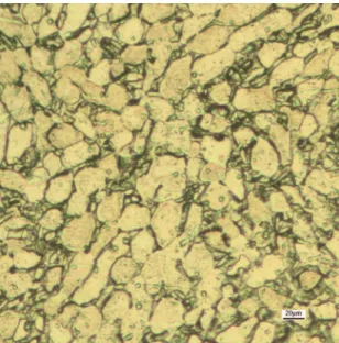
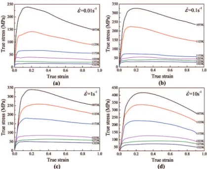
The chemical compositions (wt. %) of the adopted Ti-6Al-2Zr-1Mo-1V alloy are as follows: Al-6.30, Zr-1.9, V-1.68, Mo-1.32, Fe-0.04, C-0.01, Ni-0.01, Ti (balance). The following experimental procedures were according to ASTM Standard: E209-00. The homogenized metal bar of Ti-6Al-2Zr-1Mo-1V alloy was machined by wire-electrode cutting to several specimens with a height of 12 mm and diameter of 10 mm. Figure 1 shows the optical microstructure of the as-received Ti-6Al-2Zr-1Mo-1V alloy with single α-phase, little β-phase and negligible impurities. These specimens were compressed on a servo-hydraulic and computer-controlled Gleeble-1500 machine. The graphite lubricants were used to coat the contact surfaces of the anvils and test samples to reduce the friction and prevent bonding. The test samples were heated at a rate of 5 K/s and held at a certain temperature for 3 min to assure a uniform temperature and reduce material anisotropism. The 24 test samples were compressed with a height reduction 60% (true strain 0.9163) at the strain rates of 0.01, 0.1, 1, and 10 s-1, and the temperatures of 1073 K, 1123 K, 1173 K, 1223 K, 1273 K and 1323 K, and then these compressed test samples were rapidly quenched into water to retain the microstructures acquired at high temperatures. During these compressions, a personal computer which is equipped with an automatic data acquisition system was utilized to continuously record the nominal stress and nominal strain, and then the data were converted into true strain and true stress based on the following formulae: εT= ln 1
(
−εN)
and σT=σN(
1−εN)
,where
ε
N is the nominal strain;ε
T is the true strain;σ
T is the true stress; andσ
N is the nominal stress.Figure 2 shows the experimental true compressive stress-strain curves of Ti-6Al-2Zr-1Mo-1V alloy at diferent strain rates and temperatures. It can be summarized that the low stress level increases with the increase of strain
Figure 1: Optical photographs of the as-received Ti-6Al-2Zr-1Mo-1V alloy.
Figure 2: True stress-strain curves for Ti-6Al-2Zr-1Mo-1V alloy under diferent strain rates and temperatures.
3. Development of support vector regression
(SVR) for the low behaviors of as-cast
Ti-6Al-2Zr-1Mo-1V
In this investigation, support vector regression (SVR) was used to establish the low behaviors model of Ti-6Al-2Zr-1Mo-1V alloy on account of the excellent regression analysis ability, robustness, and high eiciency of SVR.
3.1. The basic principles of SVR
Support vector machine (SVM) is a machine learning method based on statistical learning theory and structural risk minimization principle. With the help of kernel function in SVM, the linearly inseparable low-dimensional data are mapped into linearly separable multidimensional data which can be used for classiication and regression analysis. Thereby, SVM is mainly utilized in classiication and regression analysis area, which is classiied into support vector classiication (SVC) and support vector regression (SVR).
The main advantages of SVR are as follows. Firstly, with the help of kernel function, SVR can avoid the curse of dimensionality. Secondly, in SVR, the linearly inseparable low-dimensional data are mapped into linearly separable high-dimensional data, and then SVR constructs the linear discriminant function in high dimension space to realize the nonlinear discrimination in original space. Thirdly, compared with artiicial neural network (ANN), the globally optimal solution can be obtained by using SVR. The computational process of SVR is robust and will avoid falling into local extreme value. SVR has strong generalization ability and
complete theoretical basis, and does not need to try a lot of network topologies to obtain a highly accurate model.
For a nonlinear problem, the linearly inseparable low-dimensional data are mapped into linearly separable multidimensional data by kernel function, and this mapping can be briely expressed as Eq. (1):
,
,...,
,
( )
e
e
e
e
R
R
1
n n
n n
1 1 2 2
!
!
\
U
\
U
\
U
\
U
\
U
=
Q
V
RQ
V
Q
V
Q
V
Wwhere
x
is input variable; Φ( )x is mapping function;1
e, e2 , ... , en are constants. For example, a two-dimensional data are mapped in a six dimensional space by a second-order polynomial, as expressed by Eq. (2).
,
,
1
, , , ,
,
( )
2
1 2 1 2 1 2 12 1 2 22
\ \
U
\ \
=
\ \ \ \ \ \
Q
V
Q
V
R WIn SVR, the mapping is realized by kernel function ( , )i j ( )i ( )j
k x x = Φ x ⋅ Φx . The original data can be mapped
in ininite dimensional feature space by the radial basis function (RBF), so the limited data in this feature space can be linearly separated. And a SVR equipped with the RBF can achieve a higher regression precision. Therefore, the RBF expressed as Eq. (3) was used in this investigation.
,
exp
,
( )
k
i i2
1
3
2
2
<
<
\ \
c \
\
c
x
=
-
-
=
Q
V
Q
V
where
γ
and τ2 are variable parameters of the RBF. An appropriate parameter τ2 will avoid under-itting andover-itting of data in SVR.
exist severe over-itting in the following cases: (a) penalty factor C-value is set as a certain value and 2
0
τ → ; (b) τ2 is set as a certain value and C→ ∞36. And there exist severe under-itting in the following cases: (a) C is set as a certain value and τ → ∞2 ; (b)
C is set as a smaller value and 2
0
τ → ; (c) τ2
is set as a certain value and C→036. (3) The insensitive loss function ζ .
In SVR, the ζ-value inluences the number of support vector and further impacts the regression precision of the model.
It can be summarized that the complexity, learning ability, and generalization ability of SVR depend on the three parameters
C, γ, and
ζ
, especially the mutual inluence among the three parameters. In parameters selection of SVR, optimizing each parameter is unreasonable and time-consuming. The efect of the combination of the three parameters (C, γ , andζ
) on the complexity, learning ability, and generalization of SVR should be synthetically considered. It is ineicient to manually adjust thethree parameters one by one to establish an accurate SVR in characterizing the hot low behaviors for Ti-6Al-2Zr-1Mo-1V alloy. Therefore, it is very important to ind a precise, stable and eicient method to realize the optimal selection of the three parameters in SVR. A SVR with suitable parameters C,γ
, and ζ will accurately learn the stress-strain curves and appropriately ignore some singular points of stress-strain data to accord with the overall trend of the stress-strain curves.3.3. The stress prediction model based on SVR
and Genetic Algorithm (GA)
In this section, Genetic Algorithm (GA) was combined with SVR to establish the low stress prediction model of the hot low behaviors of Ti-6Al-2Zr-1Mo-1V alloy where GA was used to eiciently search the optimal parameters combination of the three parameters (C,
γ
, and ζ), and the model was called as GA-SVR in this work.3.3.1 The basic principles of GA
Genetic Algorithm is a bionic algorithm in solving complex global optimization problem, which was enlightened by the Darwin’s natural selection theory and the genetic variation theory37. GA, as a global optimization algorithm, has widely used in various ields on account of the advantages of strong robustness, high eiciency, and parallel processing.GA seeks the optimal solution in solution space by imitating the natural selection process and natural genetic mechanism.
In GA, a population is composed of a certain number of individuals which are encoded by gene encoding.After generation of initial population, optimal approximate solutions are evolved in every generation. The individuals are selected by using itness function in each generation. According to the itness value of each individual, the individual which has a
( )
f
Q V
\
=
~ \
$
+
b
4
where
ω
is a multidimensional column vector;b is a bias term. Assuming that the original data are
1 1 2 2 3 3
( , ),( , ),( , ),...,( , ),...,( , ), ,x y x y x y x yi i x yl l x yi i∈R
. It is assumed that a function f x( ) is able to estimate all data, and the optimal function can be expressed as:
( )
min
2
1
w
C
*5
i i
i l
2
1
<
<
+
p
+
p
=
Q
V
/
. .
,
( )
s t
y
b
b
y
0
6
* *i i i
i i i
i i
$
$
#
#
$
~ \
g
p
~ \
g
p
p p
-
-
+
+ -
+
Z
[
\
]]
]]]
]]
]]
where ξi and
*
i
ξ are slack variables which can improve regression precision;
ω
is a multidimensional column vector;C is the penalty factor; ζ is an insensitive loss parameter which greatly impacts regression precision of SVR. In this work, the input variables
x
of SVR contain strain (ε), strainrate (ε̇) and temperature (T), and the target output f x( ) is low stress (σ) of Ti-6Al-2Zr-1Mo-1V alloy.
The regression function of this optimal hyperplane in SVR can be expressed as Eq. (7):
,
( )
f
i *ik
b
7
i l
i 1
\
=
a
-
a
\ \
+
=Q
V
/
Q
V
Q
V
where αi is Lagrange multiplier; b is a bias term;
( , )i
k x x is a kernel function.
3.2. The inluence of parameters selection on the
performance of SVR
In SVR, the learning performance and prediction performancecan be improved by proper parameters settings, and such parameters are penalty factor C (expressed by Eq.
(5)), the kernel parameter γ (expressed by Eq. (3)), and insensitive loss function
ζ
(expressed by Eq. (6)).(1) Penalty factor C
The complexity and robustness of SVR are inluenced by the penalty factor C-value. A larger C-value in SVR indicates
that all of data samples are important and each sample in optimal hyperplane should be correctly classiied, which will cause the model to be complex and over-itting. While a smaller C-value in SVR indicates that some singular points
can be ignored. However, if the penalty factor C-value is too small, the SVR will show the phenomenon of under-itting. (2) The parameter
γ
of basis kernel function (RBF). The RBF expressed as Eq. (3) was used in this investigation. The parameter τ2higher itness value is inherited to the next generation with greater probability. And the individuals cross and mutate to generate new population which represents new solution. The subsequent generated populations will adapt to environment better than the populations in previous generations. The best individual of last population after decoding is outputted as an approximate optimal solution.
3.3.2. The establishment of stress prediction
model GA-SVR
In order to utilize the advantages of GA, it was combined with SVR to establish the low stress prediction model of the hot low behaviors of Ti-6Al-2Zr-1Mo-1V alloy where GA was used to eiciently search the optimal parameters combination of the three parameters (C, γ , and ζ), namely, the GA-SVR.
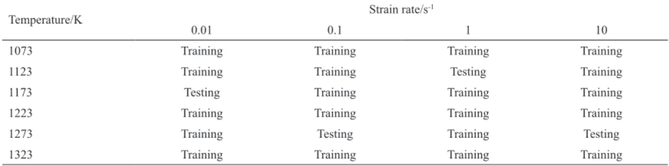
In this work, the 24 stress-strain curves were separated into two datasets, namely, the training dataset and independent test dataset, as shown in Table 1. The 864 input-output pairs were selected from the stress-strain curves to train and test the GA-SVR. The 36 stress points of the testing stress-strain curvesat the strain range of 0.1-0.9 with a distance of 0.1 were not utilized for training but for testing the generation ability of the GA-SVR. The 820 stress points of the training stress-strain curves at the strain range of 0.1-0.9 with a distance of 0.02 were utilized to train the GA-SVR. And the 8 stress points of the testing stress-strain curves at strain of 0.12 and 0.88 were used to train the GA-SVR.
The cross validation method, an efective method in evaluating the accuracy of data mining and machine learning, was utilized in this investigation to evaluate the accuracy of the established GA-SVR. In cross validation method, the original data are divided into N data sets. A separate sample is retained as a validation value and the other (N-1) samples
are used to train the GA-SVR. Each sample of N data sets is alternately set as validation data, and the performance of the GA-SVR is evaluated by the average number of the calculated evaluation index inN validation process. In this work, the number N was set as 5. An evaluation index
mean square error (MSE) between training stress data and validation stress data was introduced as Eq. (8).
where f x( )i are the predicted stress data; yi are the experimental stress data. And N is the number of stress-strain samples of validation stress dataset.
Besides, other evaluation index correlation coeicient (R) expressed as Eq. (9) was utilized to estimate degree
of correlation between the experimental low stresses and predicted low stresses38. A larger R-value demonstrates a well correlation between the two variables, and vice versa.
Table 1: The partition of training dataset and test dataset of stress-strain curves.
Temperature/K Strain rate/s
-1
0.01 0.1 1 10
1073 Training Training Training Training
1123 Training Training Testing Training
1173 Testing Training Training Training
1223 Training Training Training Training
1273 Training Testing Training Testing
1323 Training Training Training Training
( )
MSE
N
1
f
iy
i8
i N 1 2
\
=
-=
Q V
" %
/
( )
R
E
E
P
P
E
E
P
P
9
i i i
N i N i i i N 2 2 1 1 1
=
-
--
-= = =Q
Q
Q
Q
V
V
V
V
/
/
/
where E is the sample of experimental stress-strain
data; P is the sample of predicted stress-strain data; N is the number of samples of testing dataset.
The speciic lowchart of the GA-SVR was illustrated in Figure 3.
Step 1. Initialize the population of the GA-SVR. The parameters of the C,
γ
, andζ
were encoded to the chromosomes. In this investigation, the binary encoding was adopted to express individuals, because the processes of encoding and decoding operation, crossover operation, and mutation operation in binary encoding are eicient. And the binary encoding is easily analyzed by schema theorem. Here, the population number was set as 20.Step 2. The itness values of the individuals were calculated by itness function expressed by Eq. (8) in GA.
Step 3. The population was updated by the operators of selection, crossover, and mutation. According to the itness value of each individual, the individual which has a smaller
MSE-value was inherited to the next generation with greater
probability. Crossover probability PC-value is generally set in the range of 0.6 to 0.9. A larger PC-value will quickly
bring new chromosomes to the population, however, it will increase the risk of premature convergence and the loss of excellent gene structure. While a smaller PC-valuewill delay genetic evolution process. Here, the PC-valuewas set as 0.7. When the searching space of GA adjoins the optimal solution by using the crossover operator, the local random search ability of the mutation operator can be used to accelerate the convergence of the optimal solution, thereby, the mutation probability Pm-value should be set as a smaller value. Here,
4.1. The existing improved Arrhenius-type
constitutive model and ANN for as-cast
Ti-6Al-2Zr-1Mo-1V alloy
The original Arrhenius-type constitutive model expressed as Eq. (10) does not consider the inluence of strain. Afterwards, Quan et al. calculated the improved Arrhenius-type constitutive model for as-cast Ti-6Al-2Zr-1Mo-1V alloy in the reference8, which was incorporated with the inluence of strain, as expressed by Eq. (11).
Figure 3: The speciic lowchart of the GA-SVR.
Step 4. Stop criterion. If the iteration times achieves the predetermined times, the process of GA-SVR was stopped, and then the optimal parameters were used to train the GA-SVR. Otherwise, the cyclic process as shown in Figure 3 will constantly proceed. Here, the iteration times was set as 100.
Figure 4 shows the best itness value and average itness value corresponding to iteration times of the well trained GA-SVR. As shown in Figure 4, it can be observed that the convergence speed of the well trained GA-SVR is fast. In the irst 10 iteration times, the average itness value is approaching to the best itness value state. After the follow-up micro adjustments, the average itness values eventually achieve the best itness values in 10 to 20 iteration times. The C,
γ
, andζ
of the best parameters combination (R=0.999850)are 99.61, 26.19, and 0.08, respectively.
Figure 4: The relationship between the itness values and the iteration times of the GA-SVR.
4. Comparisons of the improved
Arrhenius-type constitutive model, ANN, and GA-SVR
In this chapter, the study abilities, generation abilities, and modelling eiciencies of the existing improved Arrhenius-type constitutive model, ANN, and GA-SVR for as-cast Ti-6Al-2Zr-1Mo-1V alloy were detailedly compared.
/ . / . ( ) ln exp exp A Q T A Q T 1 8 314 8 314 1 10 n n 1
2 12
v a f f = + + o o T T
Q
Q
V
V
Y Y#
&
Z [ \ ]] ]] ]] ]] ]] ]] _ a bb bb bb bb bb bbwhere
σ
is low stress (MPa) for a certain strain;T
is temperature (K); Q andA
are the activation energy (kJ·mol-1) and structure factor of Ti-6Al-2Zr-1Mo-1V alloy, respectively; α and n are the material constants of Ti-6Al-2Zr-1Mo-1V alloy.where f(ε), g(ε), h(ε), j(ε) are multinomial functions of
strain for A,
α
,n, andQ, respectively, as shown in Eq. (12).
( ) ln
Q B B B B B B B
n C C C C C C C
A D D D D D D D
E E E E E E E
12
0 1 2 2 3 3 4 4 5 5 6 6
0 1 2 2 3 3 4 4 5 5 6 6
0 1 2 2 3 3 4 4 5 5 6 6
0 1 2 2 3 3 4 4 5 5 6 6
f f f f f f
f f f f f f
f f f f f f
a f f f f f f
= + + + + + + = + + + + + + = + + + + + + = + + + + + + Z [ \ ]] ]] ]] ]] ]] ]]
where B0,B1, … ,B6, C0,C1,…,C6,D0,D1,…,D6,and E0,
E1, …,E6 are thecoeicients of the polynomial for Q, n, ln
A,and α, respectively.
Quan et al. established the ANN for as-cast Ti-6Al-2Zr-1Mo-1V alloy in the reference8.
4.2. Comparisons of the study abilities of ANN
and GA-SVR
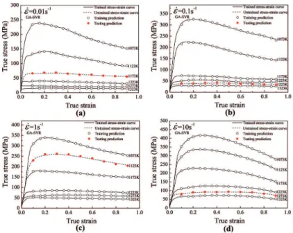
Figure 5 shows the comparisons between the trained low stresses and testing low stresses predicted by the GA-SVR at diferent strain rates and temperatures. As shown in Figure 5, the training predictions accurately track the trained stress-strain curves in a wide temperature range, stress-strain range, and strain rate range. And the testing predictions also track the trends of the untrained stress-strain curves. The correlation
/ . / . ( ) ln exp exp g f j T f j T 1 8 314 8 314 1 11 h h 1
2 21
Figure 5: Comparisons between the trained low stresses and testing low stresses predicted by the GA-SVR at diferent strain rates and temperatures of (a) 0.01 s-1, 1073-1123 K, (b) 0.1 s-1, 1073-1123 K, (c) 1 s-1, 1073-1123 K and (d) 10 s-1, 1073-1123 K.
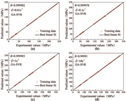
between the trained| low stresses andtraining predictions for the training dataset of the GA-SVR at (a) 0.01 s-1, (b) 0.1 s-1, (c) 1 s-1, and (d) 10 s-1 were calculated and shown in Figure 6. As exhibited in Figure 6, the R-values between the training samples and itted values of the GA-SVR model are larger than 0.9999, and there is no singular point. It can be concluded that the GA-SVR can accurately learn the highly non-linear low behavior.
In order to further estimate the study abilities of these prediction models, average absolute relative error (AARE)
was introduced. AARE is an average number of the absolute value of relative errors (δ-values).Relative error (δ) expressed by Eq. (13) is a typical evaluation index to relect diference between training data and predicted data. Compared with the δ-value, AARE expressed by Eq. (14) can better relect
prediction error, because the positive and negative δ-value cannot be ofset.
are larger than 0.9999. It can be summarized that both the ANN and GA-SVR model can suiciently and accurately learn the hot low behaviors of Ti-6Al-2Zr-1Mo-1V alloy.
4.3. Comparisons of the generalization abilities
of the improved Arrhenius-type constitutive
model, ANN, and GA-SVR
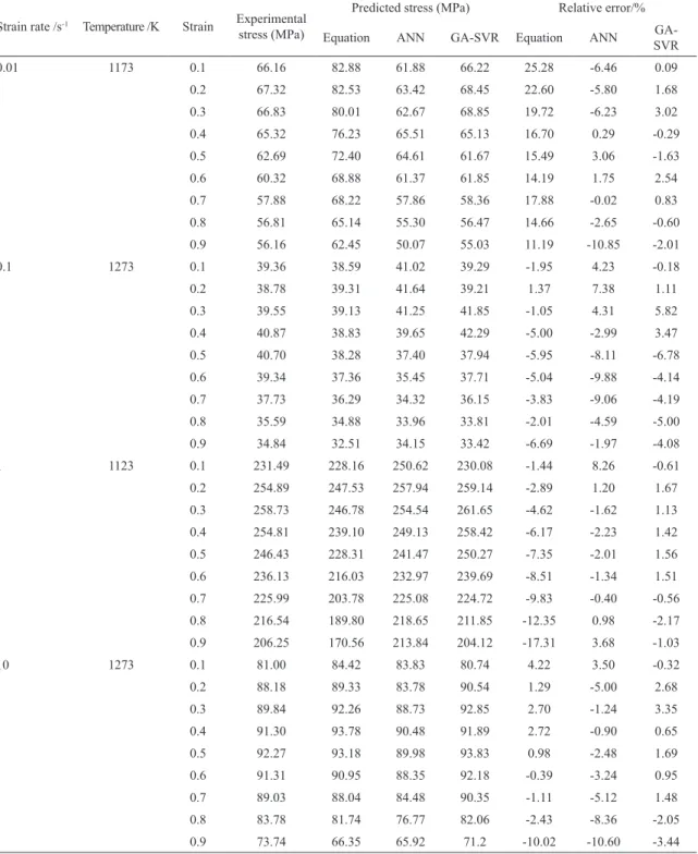
The δ-values between the experimental stress-strain data and testing stress-strain data which were predicted by the improved Arrhenius-type constitutive model, ANN, and GA-SVR were illustrated in Table 3. From Table 3, it can be found that the δ-values acquired from the improved Arrhenius-type constitutive model, ANN, and GA-SVR vary from -17.31% - 25.28%, -10.85% - 8.26%, and -6.78% - 5.82%, respectively. It is worth noting that a wider luctuation range of δ-values does not signify poor prediction performance, and the distribution and relative frequency of
δ-values should be further analyzed by Gaussian distribution analysis. After Gaussian distribution analysis, the mean number of all relative errors and standard deviation (w) can
be obtained. The -value expressed by Eq. (15) is the mean number of all relative errors. The standard deviation (w)
expressed by Eq. (16), as an evaluation index to measure discrete degree of individual in the dataset, was introduced to measure the distribution of the relative error (δ). Here, a small w indicates that most of δ-values are close to -value, and vice versa. And a smaller µ-value indicates that more predicted stress data approach the experimental stress data.
%
E
E
P
100
% ( )
13
i
i i
#
d
Q V
=
-where E is the sample of experimental stress-strain
data; P is the sample of predicted stress-strain data; N is the number of samples of testing dataset.
The R-values and AARE-values between the training samples and itted values of the ANN and GA-SVR were listed in Table 2.
As illustrated in Table 2, it can be observed that the
R-values between the training samples and itted value of
the ANN and GA-SVR model at 0.01 s-1, 0.1 s-1, 1 s-1, 10 s-1
( )
AARE
N
1
E
E
P
14
i
i i
i N
1
=
-=
/
( )
N
1
15
i i
N
1
n
=
d
=
Figure 6: Correlation between the trained low stresses and training predictions for the training dataset of the GA-SVR model of (a) 0.01
s-1, (b) 0.1 s-1, (c) 1 s-1, and (d) 10 s-1.
Table 2:R-values and AARE-values between the training samples and itted values of the ANN and GA-SVR at 0.01, 0.1, 1, and 10 s-1.
Strain rate/s-1 R-value AARE-value
ANN GA-SVR GA-SVR
0.01 0.99997 0.999982 0.6942%
0.1 0.99999 0.999978 0.2306%
1 0.99997 0.999983 0.2384%
10 0.99998 0.99991 0.1498%
Average 0.999978 0.999963 0.3282%
( )
w
N
1
1
i16
i N
2 1
d
n
=
-
-=
Q
V
/
Q
V
where δ is the sample of relative error; µ is the average number of δ-values; N is the number of samples of testing dataset.
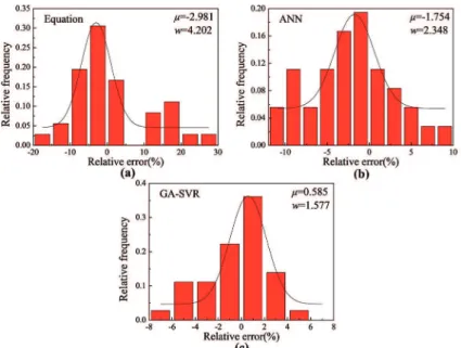
Figure 7a, b, and c show the histogram of δ-values of the improved Arrhenius-type constitutive model, ANN, and GA-SVR, respectively, which show the relative frequency of each δ-level. The µ-value and
w-value of the improved Arrhenius-type constitutive model, ANN, and GA-SVR are -2.981 & 4.202, -1.754 & 2.348, and 0.585 & 1.577, respectively. A smaller
w-value indicates that most of δ-values are close to the -value, and a smaller µ-value indicates that more predicted stress data approach the experimental stress data. It can be summarized that the generation ability of improved Arrhenius-type constitutive model is the worst, and the generation abilities of the ANN and GA-SVR are at higher levels.
Table 4 exhibits the R-values and AARE-values of test datasets of Arrhenius-type constitutive model,
ANN, and GA-SVR. The AARE-values of the improved Arrhenius-type constitutive model, ANN, and GA-SVR are 7.9703%, 4.2163894.2164%, and 2.1033%, respectively. It can be summarized that the GA-SVR has larger R-value and lower AARE-value, which indicate that the GA-SVR can accurately predict the highly non-linear flow behaviors. The generation abilities of these models were shown as follows in ascending order: the improved Arrhenius-type constitutive model < ANN < GA-SVR. The improved Arrhenius-type constitutive model cannot accurately track the hot flow behaviors, because the mathematical regression method is difficult to describe the complicated non-linear flow behaviors which accompanied with phase transformation, WH, DRV, and DRX in wide temperature and strain rate intervals. Quan et al. established the ANN model for as-cast Ti-6Al-2Zr-1Mo-1V alloy with high R-value and small
AARE-value , however, the input variables just contain
Table 3: Comparisons between experimental low stresses and predicted low stresses for test dataset.
Strain rate /s-1 Temperature /K Strain Experimental stress (MPa)
Predicted stress (MPa) Relative error/%
Equation ANN GA-SVR Equation ANN SVR
GA-0.01 1173 0.1 66.16 82.88 61.88 66.22 25.28 -6.46 0.09
0.2 67.32 82.53 63.42 68.45 22.60 -5.80 1.68
0.3 66.83 80.01 62.67 68.85 19.72 -6.23 3.02
0.4 65.32 76.23 65.51 65.13 16.70 0.29 -0.29
0.5 62.69 72.40 64.61 61.67 15.49 3.06 -1.63
0.6 60.32 68.88 61.37 61.85 14.19 1.75 2.54
0.7 57.88 68.22 57.86 58.36 17.88 -0.02 0.83
0.8 56.81 65.14 55.30 56.47 14.66 -2.65 -0.60
0.9 56.16 62.45 50.07 55.03 11.19 -10.85 -2.01
0.1 1273 0.1 39.36 38.59 41.02 39.29 -1.95 4.23 -0.18
0.2 38.78 39.31 41.64 39.21 1.37 7.38 1.11
0.3 39.55 39.13 41.25 41.85 -1.05 4.31 5.82
0.4 40.87 38.83 39.65 42.29 -5.00 -2.99 3.47
0.5 40.70 38.28 37.40 37.94 -5.95 -8.11 -6.78
0.6 39.34 37.36 35.45 37.71 -5.04 -9.88 -4.14
0.7 37.73 36.29 34.32 36.15 -3.83 -9.06 -4.19
0.8 35.59 34.88 33.96 33.81 -2.01 -4.59 -5.00
0.9 34.84 32.51 34.15 33.42 -6.69 -1.97 -4.08
1 1123 0.1 231.49 228.16 250.62 230.08 -1.44 8.26 -0.61
0.2 254.89 247.53 257.94 259.14 -2.89 1.20 1.67
0.3 258.73 246.78 254.54 261.65 -4.62 -1.62 1.13
0.4 254.81 239.10 249.13 258.42 -6.17 -2.23 1.42
0.5 246.43 228.31 241.47 250.27 -7.35 -2.01 1.56
0.6 236.13 216.03 232.97 239.69 -8.51 -1.34 1.51
0.7 225.99 203.78 225.08 224.72 -9.83 -0.40 -0.56
0.8 216.54 189.80 218.65 211.85 -12.35 0.98 -2.17
0.9 206.25 170.56 213.84 204.12 -17.31 3.68 -1.03
10 1273 0.1 81.00 84.42 83.83 80.74 4.22 3.50 -0.32
0.2 88.18 89.33 83.78 90.54 1.29 -5.00 2.68
0.3 89.84 92.26 88.73 92.85 2.70 -1.24 3.35
0.4 91.30 93.78 90.48 91.89 2.72 -0.90 0.65
0.5 92.27 93.18 89.98 93.83 0.98 -2.48 1.69
0.6 91.31 90.95 88.35 92.18 -0.39 -3.24 0.95
0.7 89.03 88.04 84.48 90.35 -1.11 -5.12 1.48
0.8 83.78 81.74 76.77 82.06 -2.43 -8.36 -2.05
0.9 73.74 66.35 65.92 71.2 -10.02 -10.60 -3.44
4.4. Comparisons of the modelling eiciencies
among the improved Arrhenius-type
constitutive model, ANN, and GA-SVR
Table 5 shows the time in modelling an accurate model of the improved Arrhenius-type constitutive model, ANN and GA-SVR. The improved Arrhenius-type constitutive model needs to calculate manymaterial constants and
Figure 7: Distribution of relative errors of test data corresponding to the (a) improved Arrhenius-type constitutive model, (b) ANN, and (c) GA-SVR.
Table 4:R-values and AARE-values of test dataset of the improved Arrhenius-type constitutive model, ANN, and GA-SVR.
R-value AARE-value
Arrhenius-type ANN GA-SVR Arrhenius-type ANN GA-VR
0.993437 0.998309 0.999676 7.9703% 4.2164% 2.1033%
Table 5: The time in modelling an accurate model of the Arrhenius-type constitutive model, ANN, and GA-SVR.
Model Arrhenius-type ANN GA-SVR
The time in modelling an accurate model. More than 180 min More than 60 min About 15 min
ANN needs to try a lot of network topologies and training parameters to obtain an accurate model, which will consume much time and energy. In addition, ANN is not very stable. To a certain dataset, the same network topology and training parameters of an ANN will obtain luctuant accuracies in diferent attempts, which reduces the modelling eiciency. Based on the operators of selection, crossover, and mutation, the GA-SVR can self-adaptively and dynamically adjust the processes of selection, crossover, and mutation to realize the optimal selection of the three parameters, which greatly improves the computational eiciency. Compared with ANN, the globally optimal solution can be obtained by using GA-SVR, and the computational processes of GA-SVR are robust and will avoid falling into local extreme value. GA-SVR does not need to try a lot of network topologies to obtain a highly accurate model. GA-SVR only needs representative training samples from the research, and then automatically adjust the three parameters C,
γ
, andζ
to obtain the most accurate prediction model. Compared with ANN, GA-SVR greatly improves the modeling eiciency. The modeling eiciencies of these models were shown as follows in ascending order: the improved Arrhenius-type constitutive model < ANN < GA-SVR.5. Applications of the GA-SVR in material
computations
5.1. Stress-strain data expansion by the GA-SVR
In this section, the low stress data at temperatures of 1098 K, 1148 K, 1198 K, 1248 K, and 1298 K under strain rates of 0.01 s-1, 0.1 s-1, 1 s-1 and 10 s-1 were predicted for Ti-6Al-2Zr-1Mo-1V alloy by the GA-SVR, as shown in Figure 8. The expanded stress-strain data are conducive to the accuracy improvement in the following ields.
5.2. Accuracy improvement in Finite Element
Modeling (FEM)
Figure 8: The true stress-strain curves of Ti-6Al-2Zr-1Mo-1V alloy under diferent temperatures and diferent strain rates where the solid curves are experimental data and the itted curves by points are predicted data.
In this section, the inluences of input stress-strain curves on simulation results were analyzed in the isothermal compression experiment by a popular FEM software DEFORM. The simulation parameters were set according to the actual experiment. One half of the specimen was simulated on account of geometric symmetry, so as to decrease the computing time. In the actual experiments, the top and bottom surfaces of specimens were coated with graphite lubricants to decrease friction between the specimen and anvils, therefore, the friction type between the contact surfaces of specimen and dies was set as shear-type in DEFORM. And a shear friction coeicient of 0.3 was set to simulate the actual graphite lubricant condition between the specimens and anvils39. In the FEM simulations, the thermal conduction and thermal radiation among compression sample, dies, and ambient were ignored to simulate the experimental isothermal compression test.
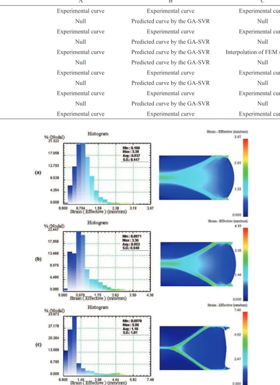
Table 6 shows three simulation schemes which were used to analyze the inluences of input stress-strain curves on inal simulation results. The entire initial conditions were selfsame except for the diferent input stress-strain curves. The compression tests were simulated at the temperature of 1173 K and strain rate of 0.01 s-1. The entire experimental stress-strain curves were inputted to the FEM software in Scheme-A, and there is no interpolation interval in scheme-A. The experimental stress-strain curves and the stress-strain curves predicted by the GA-SVR were applied to scheme-B. The experimental stress-strain curves at temperatures of 1073 , 1123, 1223, 1273, and 1323 K and strain rate of 0.01 s-1 were adopted by scheme-C, so the stress-strain curve at temperature of 1173 K and strain rate of 0.01 s-1 needs to be interpolated, and the interpolation interval was 100 K.
Figure 9b displays the distribution of effective strain of scheme-B, which can be roughly divided into three districts. The distribution of effective strain of scheme-B is similar to scheme-A, and the average strain of scheme-B is 0.953 approaching to scheme-A. Figure 9c displays the distribution of effective strain of scheme-C, which can be similarly divided into three districts. However, there are large differences of effective strain distributions between scheme-C and scheme-A, as well as the maximum effective strain. Besides, the shape of the compression sample of scheme-C is not a typical drum-type on account of the bad interpolation in a wide interpolation interval.
Additionally, as exhibited in Figure 10, the load curves corresponding to strokes of the top dies of these schemes show that the load curves of top dies of scheme-B and scheme-A are very close. The load curves of top dies of scheme-B and scheme-A are close to the experimental loads. However, there are large diferences of top die loads between scheme-C and scheme-A. The relative errors of the top die loads between scheme-A and scheme-B are in the range of -1.3818% - 2.3872%, whereas this errors between scheme-A and scheme-C are in the range of 0.7158% - 34.2327%.
Table 6: The three inite element simulation schemes at the strain rate of 0.01 s-1 and temperature of 1173 K. Temperature (K) Finite element simulation schemes
A B C
1073 Experimental curve Experimental curve Experimental curve 1098 Null Predicted curve by the GA-SVR Null 1123 Experimental curve Experimental curve Experimental curve 1148 Null Predicted curve by the GA-SVR Null
1173 Experimental curve Predicted curve by the GA-SVR Interpolation of FEM software 1198 Null Predicted curve by the GA-SVR Null
1223 Experimental curve Experimental curve Experimental curve 1248 Null Predicted curve by the GA-SVR Null 1273 Experimental curve Experimental curve Experimental curve 1298 Null Predicted curve by the GA-SVR Null 1323 Experimental curve Experimental curve Experimental curve
Figure 9: Distributions of efective strain for (a) scheme-A, (b) scheme-B, and (c) scheme-C, at the strain rate of 0.01s-1, the temperature of 1173 K, and the height reduction of 60%.
inaccurate simulation results will result in huge economic losses. It can be concluded that the GA-SVR can predict low stress data and reduce the interpolation interval to enhance the simulation accuracy.
5.3. Construction of three-dimensional (3D) low
stress map
Figure 10: The relationship between the stroke and the loads of top die for these three schemes and experimental values.
map of stress data corresponding to temperature and strain under constant strain rates8. In this work, the stress data at temperatures of 1098 K, 1148 K, 1198 K, 1248 K, and 1298 K under strain rates of 0.01 s-1, 0.1 s-1, 1 s-1 and 10 s-1 were predicted for Ti-6Al-2Zr-1Mo-1V alloy by the well-trained GA-SVR. Based on the existing experimental stress data and densely predicted stress data, a novel 3D continuous relationships among low stress, temperature, strain, and strain rate were constructed in Matlab, as shown in Figure 11. Compared with the traditional 2D stress-strain curves, the novel 3D maps of stress data are continuous and can show low stress data at any strain, strain rate
Figure 11: The (a) three-dimensional stress map and the cross sections at diferent (b) temperatures, (c) strain rates and (d) strains.
and temperature. As shown in Figure 11, the stress data are displayed by diferent colors. The X-axis, Y-axis and Z-axis coordinates represent temperature, strain rate and strain, respectively. Figure 11b-d are cross sections of Figure 11a in three orientations. Figure 11b shows the low stress data corresponding to any strain and strain rate at several ixed temperatures. In can be seen that the stress level increases with the increase of strain rate at a ixed strain, which cannot be visually demonstrated in the traditional 2D stress-strain curves. Figure 11c exhibits the stress data corresponding to any strain and temperature at several ixed strain rates, and it shows that the stress level decreases with increasing temperature at a ixed strain. Figure 11d displays the corresponding stress data to any strain rate and temperature at several ixed strains.
6. Conclusions
The novel prediction model GA-SVR was established to characterize the hot low behaviors of Ti-6Al-2Zr-1Mo-1V alloy according to the experimental stress-strain data. Following conclusions were concluded from the current study:
(1) The complexity, learning ability, and generalization ability of SVR depend on the three parameters C, γ , and ζ , especially the mutual inluence among the three parameters. The SVR with suitable parameters C, γ , and
ζ
will accurately learn the stress-strain curves and appropriately ignore some singular points of stress-strain data to accord with the overall trend of the stress-strain curves.(2) The average R-value & AARE-value between the training samples and itted values of the GA-SVR is 0.999963 & 0.3282%, which show the GA-SVR model can suiciently and accurately learn the hot low behaviors which accompany with WH, DRX and DRV. Comparison results show that the study ability of the GA-SVR is as strong as the ANN.
(3) In the comparisons of generation abilities of these models, the GA-SVR has larger R-value and lower AARE -value, which indicate that the GA-SVR can accurately predict the highly non-linear low behaviors of Ti-6Al-2Zr-1Mo-1V alloy. The generation abilities of these models were shown as follows in ascending order: the improved Arrhenius-type constitutive model < ANN < GA-SVR.
(4) Based on the operators of selection, crossover, and mutation, the GA-SVR can self-adaptively and dynamically adjust the processes of selection, crossover, and mutation to realize the optimal selection of the three parameters, which greatly improves the computational eiciency. The modeling eiciencies of these models were shown as follows in ascending order: the improved Arrhenius-type constitutive model < ANN < GA-SVR.
(5) The low behaviors under diferent temperature ranges of a material are highly non-linear, therefore, calculating stress data by interpolation method in FEM software is inaccurate. The GA-SVR can predict low stress data and reduce the interpolation interval to enhance the simulation accuracy without resorting to time-consuming and high-cost experiments. The continuously 3D relationships among low stress, temperature, strain, and strain rate were constructed, which can improve the related research ields where stress-strain data play important roles, such as improving the accuracy of inite element simulation result, improving processing maps, characterizing dynamic recrystallization evolution, etc.
7. Acknowledgements
This work was supported by National Natural Science Foundation of China (51305469). The corresponding author was also appreciated for Chongqing Higher School Youth-Backbone Teacher Support Program.
8. References
1. Wu CB, H Yang, XG Fan, ZC Sun. Dynamic globularization kinetics during hot working of TA15 titanium alloy with colony
microstructure. Transactions of Nonferrous Metals Society of China. 2011;21(9):1963-1969. http://dx.doi.org/10.1016/
s1003-6326(11)60957-6.
2. Li L, Ye B, Liu S, Hu S, Li B. Inverse analysis of the stress–strain curve to determine the materials models of work hardening
and dynamic recovery. Materials Science and Engineering: A. 2015;636:243-248. http://dx.doi.org/10.1016/j.msea.2015.03.115.
3. Quan GZ, Wang Y, Yu CT, Zhou J. Hot workability characteristics of as-cast titanium alloy Ti–6Al–2Zr–1Mo–1V: A study using
processing map. Materials Science and Engineering: A. 2013;564:46-56. http://dx.doi.org/10.1016/j.msea.2012.11.070.
4. Quan GZ, Li GS, Chen T, Wang YX, Zhang YW, Zhou J. Dynamic recrystallization kinetics of 42CrMo steel during compression at diferent temperatures and strain rates. Materials Science and Engineering: A. 2011;528(13-14):4643-4651. http://dx.doi.
org/10.1016/j.msea.2011.02.090.
5. Quan GZ, Kang BS, Ku TW, Song WJ. Identiication for the optimal working parameters of Al–Zn–Mg–Cu alloy with the
processing maps based on DMM. The International Journal of Advanced Manufacturing Technology. 2011;56(9):1069-1078.
http://dx.doi.org/10.1007/s00170-011-3241-6.
6. Lin YC, Li QF, Xia YC, Li LT. A phenomenological constitutive model for high temperature low stress prediction of Al–Cu–Mg
alloy. Materials Science and Engineering: A. 2012;534:654-662.
http://dx.doi.org/10.1016/j.msea.2011.12.023.
7. Li HY, Hu JD, Wei DD, Wang XF, Li YH. Artiicial neural network
and constitutive equations to predict the hot deformation
behavior of modiied 2.25Cr–1Mo steel. Materials & Design. 2012;42:192-197. http://dx.doi.org/10.1016/j.matdes.2012.05.056.
8. Quan GZ, Lv WQ, Mao YP, Zhang YW, Zhou J. Prediction of low stress in a wide temperature range involving phase transformation for as-cast Ti–6Al–2Zr–1Mo–1V alloy by artiicial neural network. Materials & Design. 2013;50:51-61.
http://dx.doi.org/10.1016/j.matdes.2013.02.033.
9. Guan Z, Ren M, Zhao P, Ma P, Wang O. Constitutive equations
with varying parameters for superplastic low behavior of Al–Zn– Mg–Zr alloy. Materials & Design (1980-2015). 2014;54:906-913.
http://dx.doi.org/10.1016/j.matdes.2013.09.014.
10. Fan XG, Yang H, Gao PF. Prediction of constitutive behavior
and microstructure evolution in hot deformation of TA15 titanium alloy. Materials & Design. 2013;51:34-42. http://
dx.doi.org/10.1016/j.matdes.2013.03.103.
11. Voyiadjis GZ, Abed FH. Microstructural based models for bcc
and fcc metals with temperature and strain rate dependency.
Mechanics of Materials. 2005;37(2-3):355-378. http://dx.doi.
org/10.1016/j.mechmat.2004.02.003.
12. Zhang C, Ding J, Dong Y, Zhao G, Gao A, Wang L. Identiication of friction coeicients and strain-compensated Arrhenius-type
constitutive model by a two-stage inverse analysis technique.
International Journal of Mechanical Sciences. 2015;98:195-204.
13. Lin YC, Wen DC, Huang YC, Chen XM, Chen XW. A uniied
physically based constitutive model for describing strain
hardening efect and dynamic recovery behavior of a Ni-based
superalloy. Journal of Materials Research.
2015;30(24):3784-3794. http://dx.doi.org/10.1557/jmr.2015.368.
14. Lin YC, Chen XM, Wen DX, Chen MS. A physically-based constitutive model for a typical nickel-based superalloy.
Computational Materials Science. 2014;83:282-289. http://
dx.doi.org/10.1016/j.commatsci.2013.11.003.
15. Xiao J, Li DS, Li XQ, Deng TS. Constitutive modeling and microstructure change of Ti–6Al–4V during the hot tensile
deformation. Journal of Alloys and Compounds. 2012;541:346-352. http://dx.doi.org/10.1016/j.jallcom.2012.07.048.
16. Peng W, Zeng W, Wang Q, Yu H. Comparative study on
constitutive relationship of as-cast Ti60 titanium alloy during hot deformation based on Arrhenius-type and artificial neural
network models. Materials & Design. 2013;51:95-104.
http://dx.doi.org/10.1016/j.matdes.2013.04.009.
17. Sajadifar SV, Yapici GC. Workability characteristics and
mechanical behavior modeling of severely deformed pure titanium at high temperatures. Materials & Design. 2014;53:749-757. http://dx.doi.org/10.1016/j.matdes.2013.07.057.
18. Lin YC, Chen MS, Zhong J. Prediction of 42CrMo steel
flow stress at high temperature and strain rate. Mechanics Research Communications. 2008;35(3):142-150. http://
dx.doi.org/10.1016/j.mechrescom.2007.10.002.
19. Lin YC, Li KK, Li HB, Chen J, Chen XM, Wen DX. New
constitutive model for high-temperature deformation behavior of inconel 718 superalloy. Materials & Design. 2015;74:108-118. http://dx.doi.org/10.1016/j.matdes.2015.03.001.
20. Quan GZ, Shi Y, Yu CT, Zhou J. The improved Arrhenius model with variable parameters of flow behavior characterizing
for the as-cast AZ80 magnesium alloy. Materials Research.
2013;16(4):785-791.
http://dx.doi.org/10.1590/s1516-14392013005000070.
21. Khan AS, Kazmi R, Farrokh B, Zupan M. Effect of oxygen
content and microstructure on the thermo-mechanical response
of three Ti–6Al–4V alloys: Experiments and modeling over
a wide range of strain-rates and temperatures. International Journal of Plasticity. 2007;23(7):1105-1125. http://dx.doi.
org/10.1016/j.ijplas.2006.10.007.
22. Khan AS, Suh YS, Kazmi R. Quasi-static and dynamic loading
responses and constitutive modeling of titanium alloys.
International Journal of Plasticity. 2004;20(12):2233-2248.
http://dx.doi.org/10.1016/j.ijplas.2003.06.005.
23. Kotkunde N, Deole AD, Gupta AK, Singh SK. Comparative study of constitutive modeling for Ti–6Al–4V alloy at
low strain rates and elevated temperatures. Materials & Design. 2014;55:999-1005. http://dx.doi.org/10.1016/j. matdes.2013.10.089.
24. Akbari Z, Mirzadeh H, Cabrera JM. A simple constitutive
model for predicting flow stress of medium carbon microalloyed steel during hot deformation. Materials & Design. 2015;77:126-131. http://dx.doi.org/10.1016/j. matdes.2015.04.005.
25. Liu J, Zeng W, Lai Y, Jia Z. Constitutive model of Ti17
titanium alloy with lamellar-type initial microstructure during hot deformation based on orthogonal analysis.
Materials Science and Engineering: A. 2014;597:387-394.
http://dx.doi.org/10.1016/j.msea.2013.12.076.
26. Quan GZ, Zhang ZH, Pan J, Xia YF. Modelling the Hot Flow Behaviors of AZ80 Alloy by BP-ANN and the
Applications in Accuracy Improvement of Computations.
Materials Research. 2015;18(6):1331-1345. http://dx.doi.
org/10.1590/1516-1439.040015.
27. Zhu Y, Zeng W, Sun Y, Feng F, Zhou Y. Artificial neural network approach to predict the flow stress in the isothermal
compression of as-cast TC21 titanium alloy. Computational Materials Science. 2011;50(5):1785-1790. http://dx.doi.
org/10.1016/j.commatsci.2011.01.015.
28. Lou Y, Ke CX, Li L. Accurately Predicting High Temperature Flow Stress of AZ80 Magnesium Alloy with Particle Swarm Optimization-based Support Vector Regression. Applied Mathematics & Information Sciences. 2013;7(3):1093-1102.
29. Desu RK, Guntuku SC, Aditya B, Gupta AK. Support Vector Regression based Flow Stress Prediction in Austenitic Stainless Steel 304. Procedia Materials Science. 2014;6:368-375. http://dx.doi.org/10.1016/j.mspro.2014.07.047.
30. Sun Z, Yang H, Tang Z. Microstructural evolution model of TA15 titanium alloy based on BP neural network method
and application in isothermal deformation. Computational Materials Science. 2010;50(2):308-318. http://dx.doi.
org/10.1016/j.commatsci.2010.08.020.
31. Ji G, Li F, Li Q, Li H, Li Z. A comparative study on
Arrhenius-type constitutive model and artificial neural
network model to predict high-temperature deformation
behaviour in Aermet100 steel. Materials Science and Engineering: A. 2011;528(13-14):4774-4782. http://dx.doi.
org/10.1016/j.msea.2011.03.017.
32. Mandal S, Sivaprasad PV, Venugopal S, Murthy KPN. Artificial neural network modeling to evaluate and predict the deformation behavior of stainless steel type AISI 304L
during hot torsion. Applied Soft Computing.
2009;9(1):237-244. http://dx.doi.org/10.1016/j.asoc.2008.03.016.
33. Sun Y, Zeng WD, Zhao YQ, Han YF, Ma X. Intelligent method to develop constitutive relationship of Ti–6Al– 2Zr–1Mo–1V alloy. Transactions of Nonferrous Metals Society of China. 2012;22(6):1457-1461. http://dx.doi.
org/10.1016/s1003-6326(11)61341-1.
34. Quan GZ, Wu DS, Luo GC, Xia YF, Zhou J, Liu Q et al. Dynamic recrystallization kinetics in α phase of as-cast Ti–6Al–2Zr–1Mo–1V alloy during compression at different
temperatures and strain rates. Materials Science and Engineering: A. 2014;589:23-33. http://dx.doi.org/10.1016/j. msea.2013.09.069.
35. Sakai T, Belyakov A, Kaibyshev R, Miura H, Jonas JJ. Dynamic and post-dynamic recrystallization under hot,
cold and severe plastic deformation conditions. Progress in Materials Science. 2014;60(1):130-207. http://dx.doi.
36. Keerthi SS, Lin CJ. Asymptotic behaviors of support vector machines with Gaussian kernel. Neural Computation.
2003;15(7):1667-1689.
37. Sivaraj R, Ravichandran T. An improved clustering based genetic algorithm for solving complex NP problems. Journal of Computer Science. 2011;7(7):1033-1037.
38. Chai RX, Guo C, Yu L. Two flowing stress models for hot
deformation of XC45 steel at high temperature. Materials Science and Engineering: A. 2012;534:101-110. http://
dx.doi.org/10.1016/j.msea.2011.11.047.
39. Li LX, Peng DS, Liu JA, Liu ZQ. An experiment study of
the lubrication behavior of graphite in hot compression
tests of Ti–6Al–4V alloy. Journal of Materials Processing Technology. 2001;112(1):1-5.
40. Sabokpa O, Zarei-Hanzaki A, Abedi HR, Haghdadi N. Artificial neural network modeling to predict the high
temperature flow behavior of an AZ81 magnesium alloy.
Materials & Design. 2012;39:390-396. http://dx.doi.