Assessing the influence of the scale of operations on maintenance costs in the airline
industry
Diego Javier Gonzales Vega; Daniel Alberto Pamplona+; Alessandro V. M. Oliveira Instituto Tecnológico de Aeronáutica, São José dos Campos, Brasil
Article Info Abstract
Keywords: maintenance econometric airline operations costs
economies of scale
The aim of this study is to investigate whether the size of airline operations has any statistically significant effect on the costs of its aircraft maintenance. By investigating the impact of the extent of operations on unit costs of carriers, it was inspected the existence of economies of scale in providing maintenance services. Through an econometric model of maintenance costs, it was estimated the influence of key drivers such as the aircraft average stage length, aircraft size and load factors. It was performed an application to the Brazilian airline industry. The empirical model makes use of a Fixed-Effects Estimator (FE), using a four-dimensional panel data of flight segments, carriers and equipment over a period of ten years. Results showed support for the hypothesis of scale economies in maintenance services. The academic gain of this article is through econometric analysis identify factors that influence the maintenance costs for airlines. Noting that the largest companies have lower maintenance costs (economies of scale), enables administrators and air planners a better understanding of the phenomenon, as well as a better use of the resources available. For smaller companies, outsourcing or sharing of maintenance with other companies, can result in major savings and profitability.
Submitted 9 May 2015;
received in revised form 9 Jun 2015; accepted 12 Jul 2015.
Licensed under Creative Commons CC-BY 3.0 BR.
+ Corresponding author. Instituto Tecnológico de Aeronáutica. Praça Marechal Eduardo Gomes, 50. 12.280-250 - São José dos Campos, SP - Brasil. E-mail address: [email protected]
Introduction
The objective of this study is to investigate if there is any support for an inverse relation between the size of a company and its unit cost of maintenance services in the airline industry. As the extent of operations of a carrier increases, economies of scale are expected to produce lower unit costs, especially for in-house maintenance. This effect may also be observed in vertical relations between suppliers and contractors, as bigger companies may have a more efficient negotiation power in case of maintenance contracts. The secondary objective of the paper is to analyze the formation of unitary costs in the airline industry by utilizing panel data techniques.
The survival of an airline in a competitive market environment is nowadays only accomplished with strict cost management strategies. Maintenance costs is one of the costs items that can be reasonably controlled if correctly scheduled, even though delays and unforeseen corrective maintenance are still the major uncontrollable components in the management process. With the increasing complexity of aircraft systems, the issue of maintenance has always attracted the attention of airlines and manufacturers, which are operating in one of the most competitive environments, in order to reduce or even eliminate maintenance problems (Knotts, 1999).
In this article was developed an econometric model accounting for the four dimension panel characteristics of the dataset, with the dimensions being flight segments, carriers, flight equipment and a time span of ten years. It was performed an application to the Brazilian airline industry. The econometric model of maintenance unit costs estimate the influence of key drivers such as the aircraft average stage length, aircraft size and load factors. The empirical strategy was to undertake the estimation of multiple models, beginning with the basic pooled Ordinary Least Square (OLS), and later employing panel data estimators such as the Fixed Effects Estimator (FE) and the Random Effects Estimator (RE). Hypothesis tests were provided to investigate which of these models performs better in the analysis. Results show that there is a factor that punishes smaller carriers with higher unit costs of maintenance. Results showed support for the hypothesis of scale economies in maintenance services.
The academic gain of this article is through econometric analysis; identify factors that influence the maintenance costs for airlines. Noting that the largest companies have lower maintenance costs (economies of scale), enables administrators and air planners a better understanding of the phenomenon, as well as a better use of the resources available. For smaller companies, outsourcing or sharing of maintenance with other companies, can result in major savings and profitability.
This paper is organized in the following way. First, Section 1 presents some relevant facts about maintenance costs in the airline industry along with some statistics of the sector. Section 2 contains the presentation of the data set, the econometric modeling and the discussion of results, which is followed by the conclusions.
1. Maintenance costs analysis
Worldwide, the airline industry has suffered great changes since the Airline Deregulation Act in the United States, in 1979. Several airline markets have been fully liberalized since then, with a notable intensification in competition. Due to the emergence of new technologies, the airline industry is compelled to minimize its operative costs while improving profitability in rapidly changing environment. Most of the financial problems faced by carriers in the airline industry usually originate from the cyclical, seasonal and ultimately unpredictable behavior of demand.
Besides the demand side, the high labor/capital utilization ratios, the volatile of jet fuel prices, strong labor unions are factors that contribute to the complexity of the management of any carrier nowadays (Knotts, 1999). Cost management has become a very important tool in the strategic planning of any airline. One way to operational optimization is the study of costs. Mahour et al. (2010) investigates the relation between operational factors toward airline profitability, and among others factors the hourly maintenance cost was a valuable determinant to the industry optimization. According to Zuidberg (2014), the profit margins of the majority of airlines worldwide are under constant pressure. Even in periods of high economic growth, many airlines scarcely make a profit.
Aircraft maintenance is all actions that can restore an item to a serviceable condition, and consist of servicing, repair, modification, overhaul, inspection and determination of condition. Maintenance can be classified as:
Corrective maintenance - All actions performed as a result of failure to restore an item to a satisfactory condition by providing correction of a known or suspect malfunction and/or defect. Corrective maintenance can include any or all of the following steps: defect location, defect isolation, disassembly, replacement, reassembly, alignment / adjustment, and testing. This type of maintenance is known as unscheduled maintenance.
Preventive maintenance - All actions performed at defined intervals to retain an item in a serviceable condition by systematic inspection, detection, replacement of wear out items, adjustment, calibration, cleaning etc. This type of maintenance is carried out at prescribed points in an aircraft and equipment's life and is termed scheduled maintenance.
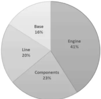
The maintenance costs for an aircraft vary with age. New aircrafts have relatively low costs associated with the airframe. However, they rise steadily, levelling off around five years of usage. After that, an aircraft has a steady, predictable maintenance cost, which begins to rise again after around 15 years, because of airframe and components age (Cook & Tanner, 2008). Maintenance costs typically account for 10-20 per cent of aircraft-related operating costs (Maple, 2001). In 2012, airlines worldwide spent $665 billion to operate, and the Maintenance, Repairs and Overhaul (MRO) market reached $46.9 billion. The amount of airline MRO spend reflects only the expected direct maintenance cost of the four maintenance market segments (line, component, engine, heavy maintenance), according to Figure 1 (IATA, 2013).
Figure 1 - Direct Maintenance Costs by Segment. Source: International Air Transport Association, 2013.
The main goal of the maintenance is to offer a fully serviceable aircraft when it is required by an airline at minimum cost. For the present, maintenance costs of commercial aircraft make a significant contribution to an aircraft’s cost of ownership. 1.1. Maintenance statistics
The data were incomplete, as data for year, 2004 for the International segment was missing. Either way, the series present stability, the maintenance cost had a lower tendency but it begin to grow as the operations also did, as consequence of the increase in flight activity of the last years. The same can be observed with the flight hours and the total trips, according to Figure 2.
Figure 2 – Maintenance costs. Source: National Agency for Civil Aviation, 2009.
Figure 3 – Unit cost of maintenance. Source: National Agency for Civil Aviation, 2009.
However, the dependent variables behave different, clearly the unitary cost as a function of the trips is more decreasing than the one with hourly flight. It is expected that the former had better performance in the estimation of models because they behave in a similar way, also because the variability will be lower, assuring good individual and global performance.
2. Econometric model of unit costs maintenance
The data were obtained from the economic yearbook of the National Agency for Civil Aviation (ANAC), for the period from 1999 to 2008. The variables chosen for the data panel are the maintenance cost, the total trips made (sum of programmed trips and extraordinary trips), the number of kilometer flown, the time of flight (in hours), the average stage length and the gross domestic production. In addition, there are information referenced to segment of flight (domestic and international), name of the airline and type of equipment with them were generated an index, which serves as time series in the data panel representation, the years are also represented as time series for further comparison of models.
The dependent variable chosen was the unitary cost of maintenance. But as mentioned, there were two ways of generate it, one as the ratio of maintenance costs and total trips, other as a ratio with flight hours, as a function of flight hour or total trips depending of the dependent variable. The control variables were clearly separated in three fields. The performance variables such as the airplane size (asize), the average stage length (avst) and the load factor (lf) are expected that these variables have positive signals. The macroeconomic variables such as the exchange rate (ers2) applied to the international segment1 should be positive. In addition, as an increase of the exchange rate had to increase the price of the machinery and the gross domestic production (gdp) being the last. The revenue passengers per airline company part of the hypothesis variables –there is a revealed preference to larger companies– thus the signal should be negative.
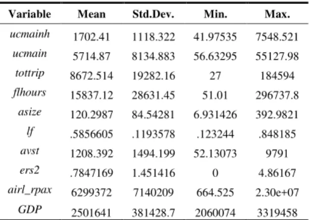
This statistic representation shows the static behavior of the variables, according to Table 1.
Table 1 - Data statistics representation. Source: With own calculations.
The variability of the hourly maintenance unitary cost is lower than the maintenance unitary cost per flight. The rest of the variables present standard deviations bigger than its mean, which show high variability, clearly explained by the presence of many companies’ sizes. Several models were tested with OLS, Fixed Effects and Random Effects Panel Data. 2.1. Econometric study and results
The first models are made on Ordinary Least Square (OLS). The model 1a estimate the unitary cost of maintenance per hour as a function of the total trips, airplane size, the load factor, the average length of flight, the exchange rate, the revenue passengers per airline and the gross domestic production. The model 1b estimate the unitary cost of maintenance per trip as a function of the flight hours, and the same others:
(1a)
(2b)
1 In order to better control, and to differentiate the internal and the external market. Variable Mean Std.Dev. Min. Max.
ucmainh 1702.41 1118.322 41.97535 7548.521
ucmain 5714.87 8134.883 56.63295 55127.98
tottrip 8672.514 19282.16 27 184594
flhours 15837.12 28631.45 51.01 296737.8
asize 120.2987 84.54281 6.931426 392.9821
lf .5856605 .1193578 .123244 .848185
avst 1208.392 1494.199 52.13073 9791
ers2 .7847169 1.451416 0 4.86167
airl_rpax 6299372 7140209 664.525 2.30e+07
The two sets of models correspond each to a form of attain a dependent variable, because now it is unknown a plausible measure of knowing the better way to choose. In order to choose the better model, it is compared the representations of both models estimated with Ordinary Least Squares, according to Table 2.
Table 2 – OLS representations. Source: With own calculations.
Superscripts *, **, and *** denote, respectively, significance at the 5%, 1% and 0.1%
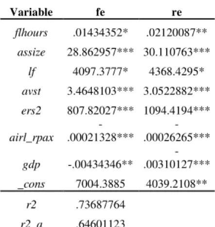
To better chose a model, it was estimated the very same model with fixed effects of the index of segment, airline and equipment. The panel data model with more than 600 values is highly restrictive as the index have nearly 160 groups. The model with fixed effects contains the same variables as the model 1b (which had better R2). This regression consider the change in the index, created from the segment, the airline and the equipment and the years. In addition, it is considered time invariant variables (index), and assumed that they can explain the behavior of the dependent variable. Then a random effects model is estimated too. Results showed that the goodness of fit is better with random effects, the model is global significant, and the parameters have similar signals and values, according to Table 3.
Table 3– Fixed and Random Effects representations. Source: With own calculations.
Superscripts *, **, and *** denote, respectively, significance at the 5%, 1% and 0.1%
The coefficients have the expected signals. The unitary cost for maintenance respond positively from the flight hours as the more the plane travel the more the maintenance of the fuselage and the engines. The airplane size because the bigger the airplane the bigger the time and equipment’s hour to maintain it. The load factor control the maintenance of the seats and the passenger environment and the average length of flight, the longer the stage, the bigger the cost of maintenance.
In the case of the gross domestic production it is possible to extrapolate that with the increase of production the total maintenance cost do the same. Nevertheless, at the same time, the capacity of negotiation of the industry increases so the unitary cost decreases.
In addition, there are companies that made its own maintenance. Nevertheless, the companies have their costs because they do not produce the spare parts, but clearly, they have to benefit in some way, thus the negative signal associated to the size of the company. The revenue passengers per airline shows that the bigger the company the lower the unitary maintenance cost, surely is a very low discount but there is one.
The models had strong single and global significance with both t and F statistics less than 5%, the values and signals of the parameters are over the expected. With this representation, we estimate the panel data models. The random effect model presented better estimates but assuming strong hypothesis of uncorrelated error, in order to reject that hypothesis the Hausman test was done, according to Table 4.
Variable OLS 1a OLS1b
tottrip .00426274*
assize 9.5577875*** 29.82527***
lf 462.90073 4295.0334*
avst -.08284325* 3.0243987***
ers2 119.06105*** 1156.8203***
airl_rpax -.00002858*** -.00027225***
gdp -.00015345 -.00308133***
flhours .02345395***
_cons 815.154** 4100.9924**
r2 .39462068 .70552838
r2_a .38787282 .70224605
Variable fe re
flhours .01434352* .02120087**
assize 28.862957*** 30.110763***
lf 4097.3777* 4368.4295*
avst 3.4648103*** 3.0522882***
ers2 807.82027*** 1094.4194***
airl_rpax
-.00021328***
-.00026265***
gdp -.00434346**
-.00310127***
_cons 7004.3885 4039.2108**
r2 .73687764
Table 4– Hausman test. Source: With own calculations.
b denotes consistent under H0 and Ha. B denotes inconsistent under Ha, efficiente under H0. For the test, H0 denotes de difference in coefficients not systematic.
With this, the hypothesis made by the random is rejected, so it was selected the fixed effects model. With this selection, it is possible to forecast the unitary maintenance costs. However, it is necessary to make further hypothesis for the evolution of the variables because the GDP have forecasts made by the Central Bank, the average length, flight hours can be extrapoled from the predictions of airline demand and the load factor, and aircraft size was assumed constant.
Conclusion
The literature keeps reminding us that bigger companies have bigger costs. It can be appreciated a different scale of increasing, hence the unitary costs should be decreasing as the quantity don’t increase at the same ratio as the costs, the size of the served net allow network carriers to benefit from differentiated location costs, the maintenance being one of them.
The focus of the study was to investigate if the size of a company has influence in the power of negotiation, which gives them economic - scale – benefit in the formation of maintenance costs, which ultimately affect in their cost structure improving the optimization and their profit, assuring their survival.
The unitary cost can be modeled with panel data approach, and is robust enough to achieve forecast with the proper assumption of the behavior of the remaining variables. Future studies should focus on the variables used in this paper such as GDP, average length of the flights, flight hours, airline demand, and load factor and aircraft size. Another limited factor is the lack of data for the year 2004 in the international segment. The study range should be expanded until presente days, and verify if the scale of operations is maintained.
As highlighted in the article, the survival of an airline in a competitive market environment is nowadays only accomplished with strict cost management strategies. Maintenance costs represents a fraction of the costs. In a rapidly changing environment, the airline industry is compelled to minimize its costs while improving profitability and safety in a rapidly changing environment.
References
Brazilian National Agency for Civil Aviation. (2008). Air Transport Handbook 2008. Brazil.
Cook, A. J., & Tanner, G. (2008). Innovative Cooperative Actions of R&D in EUROCONTROL Programme CARE INO III: Dynamic Cost Indexing: Aircraft maintenance–marginal delay costs.
International Air Transport Association - IATA. (2013). Airline Maintenance Cost: Executive Commentary. IATA.
Knotts, R. M. H. (1999). Civil aircraft maintenance and support Fault diagnosis from a business perspective. Journal of quality in maintenance engineering, 5(4), 335-348.
Maple, M. (2001). Understanding maintenance costs for new and existing aircraft. Airline Fleet and Asset Management(5), 56-62.
Mellat Parast, M., & Fini, E. H. (2010). The effect of productivity and quality on profitability in US airline industry: an empirical investigation. Managing Service Quality: An International Journal, 20(5), 458-474.
Zuidberg, J. (2014). Identifying airline cost economies: An econometric analysis of the factors affecting aircraft operating costs. Journal of Air Transport Management, 40, 86-95.
Coefficients
(b) (B) (b-B) squrt(diag(V_b-b_B))
fe re Difference S.E.
flhours .0143435 .0212009 -.0068574 .0025957
assize 28.86296 30.11076 -1.247807 1.492637
lf 4097.378 4368.43 -271.0518 964.2676
avst 3.46481 3.052288 .4125222 .1196753
ers2 807.8203 1094.419 -286.5992 88.72295
airl_rpax -.0002133 -.0002626 .0000494 .0000171
gdp -.0043435 -.0031013 -.0012422 .0012272
Prob>Χ2