Master of Science in Economics Masters Thesis

(1)

The implications of mandatory low-cost fuel provision

Master of Science in Economics Masters Thesis

Advisor:

Pedro Pita Barros

NOVASCHOOL OF BUSINESS AND ECONOMICS Fall Semester 2015/2016

by

Rodrigo Pina Cipriano

Student ID 22717

Economics

rodrigo.jp.cipriano@gmail.com

(2)

The implications of mandatory low-cost fuel provision

Abstract

This work studies fuel retail firms’ strategic behavior in a two-dimensional product

differentiation framework. Following the mandatory provision of “low-cost” fuel we

consider that capacity constraints force firms to eliminate of one the previously offered

qualities. Firms play a two-stage game choosing fuel qualities from three possibilities

(low-cost, medium quality and high quality fuel) and then prices having exogenous

opposite locations. In the highest level of consumers’ heterogeneity, a subgame perfect

Nash equilibrium exists in which firms both choose minimum quality differentiation.

Consumers’ are worse off if no differentiation occurs in medium and high qualities. The

effect over prices from the mandatory “low-cost” fuel law is ambiguous.

(3)

1 Introduction

On April 17th of 2015 new legislation imposed gas stations to provide a no-additives fuels

(“low-cost” or simple fuels) option to consumers in Portugal.1 Independently of the brand

simple fuels’ level of additives is that needed to meet minimum quality requirements

defined by law. 2 These fuels are similar to those sold by large retail chains and unbranded

operators. Over the past decade independent/unbranded gasoline stations selling exclusively

low-cost fuels have been gaining market share to branded stations. 3 Unbranded stations are

usually operated by large grocery retailers and located next to their stores while branded

stations often provide ancillary services such as car wash, tire-fill, loyalty cards, and

products of convenience. Fuels can be categorized in three segments according to its

quality: regular (simple or low-cost), medium and premium. Premium fuels are the

top-quality fuels, with the highest concentrations of additives and the simple fuels are those

with lower concentrations of additives. To justify this policy, the government argued that it

would promote competition lowering prices for the consumer and more freedom of choice.

Major branded fuel retailers’ stations criticized the measure, arguing that their business

model involves other costs that would prevent them to keep up with unbranded stations

prices for low-cost fuel.4 Another argument against the measure was the possible damage to

the freedom of choice given that capacity constraints would dictate the elimination of other

1

Law no. 6/2015:http://goo.gl/UA4mJy

2

Decree law no. 142/2010, of 31 December 3

According to the Portuguese Competition Authority between 2008 and 2013 low-cost fuels market share grew from 12% to 25%. In 2015 a study by Kantar contracted by the Portuguese Association of Distribution Companies indicates that low-cost fuels account for more than 28% of the market.

4

(4)

qualities in order to offer low quality fuel. Mandatory introduction of simple fuel and

stations’ capacity constraints forced firms to choose which of the qualities (standard or

premium) should be replaced for the former. The choice of which quality to eliminate can

be seen as a strategic one, from which a game between firms emerge. Firms decide by

anticipating other firms’ and consumers’ behavior as well as prices and profits resulting

from competitive interactions. Naturally, differences in quality, location, production costs

and consumers’ tastes influence the market dynamics. Profits will ultimately determine

which products will be available in the market.

This paper is organized as follows. In section 2 a contextualization of this paper in the

existing literature is made. Section 3 introduces a description of the different models used

to analyzed competition under two-dimensional product differentiation. In Section 4 each

model is developed. Equilibrium prices, demands and strategies’ payoffs are found and

main results are exposed.5 Finally, Section 5 presents concluding remarks.

2 Literature Review

Competition in fuel/gasoline retail market has been recurrently the core of many empirical

studies over the last decades. Most literature focus on the study of two important

phenomena: asymmetric Edgeworth price cycles and collusion behavior.6 Maskin and

Tirole (1988) first formalized the Edgeworth cycle concept, describing it as an equilibrium

where “firms undercut each other successively until the price reaches the competitive level

at which point some firm eventually reverts to the high price”. Several works (e.g., Noel,

5

For the third model further analysis regarding equilibrium prices and welfare is performed.

6

Edgeworth (1925) argued that stationary price equilibrium doesn’t take place when firms are confronted

(5)

2004; Verlinda, 2008; Noel, 2011) find proof that firms engage in Edgeworth cycles’

behavior, leading to a fast price increase and a slower price decrease stages. Others focus

on the speed of price adjustments to cost variations. Bacon (1991), Borenstein et al. (1992),

Golby et al. (2000), Johnson (2002) used significant datasets to confirm asymmetries in

price adjustments also known as “rockets rise faster and feather fall slower” events.

Borenstein (1997) explains such asymmetry with the uncertainty of competitors’ costs, but

others such as Johnson (2002) explain it with the incentives for buyers to engage more

intensively in searching prices. Relevant works also focused on tacit collusion between

firms in retail fuel markets. Such behavior may be related to asymmetric price adjustments

which provides strong reasons to study firms’ strategic behavior.7 Supported by distinct

theoretical models, important empirical works (Shepard and Borenstein, 1996; Wang, 2008;

García, 2010) provide strong evidence of collusive behavior in different fuels retail

markets.

Representing fuel market’s organization and dynamics is not an easy task. Fuels can easily

be considered to be differentiated over two dimensions: vertical and horizontal. While

literature addressing one dimensional product differentiation is extensive, works

accommodating the two dimensions are not as common. Hotelling (1929) made one of the

first attempts to model horizontal differentiation, where firms compete in a two-stage

location-price game.8 A significant number works followed further exploring

Hotelling-type models. Either by considering a circular city, free entry and large number of firms as

Salop, 1979) or key calculations’ corrections and quadratic transportation costs

7

Clark and Houde (2011) identified evidence of asymmetric pricing cycles being an important feature associated with a price-fixing cartel.

8_{First choosing locations (in a unitary “linear city”) and then p}

(6)

(d’Aspremont et al. 1979) location models have been widely used. Concerning the vertical

dimension Gabszwicz and Thisse (1979, 1980) tried to “capture an important fact of life:

the quality component of the choice in economic decisions” accommodating consumers’

with similar tastes but distinct income and firms with substitute products competing in the

same market. Shaked and Sutton (1982) extended the exercise by considering a previous

stage where two firms choose or not to enter the market and then to decide on maximal or

minimal quality differentiation.9 Similarly to location models, in quality differentiation

usual results show differentiation being a way to soften price competition and exploit

consumers’ surplus. Some literature has developed competition models encompassing both

vertical and horizontal dimensions. Economides (1989) analyses a sequential game of

variety(location)-quality-price choices to find evidence of maximally differentiated

varieties but minimal differentiation on the other dimensions. This result is consistent with

that of Irmen (1988) –firms identify a dominant dimension to maximally differentiate in

while minimum differentiation holds for all other dimensions.10 Other literature also

provides interesting results in the two-dimensional framework but do not closely relate to

the scope of this work.11 Although with significant similarities in what concerns to models

specification to my best knowledge none of the existing literature focuses on firms’

decisions about quality differentiation arising from both public intervention and capacity

constraints – the core issue of the present document.

9

Results yielded both firms entering the market and producing differentiated products which would allow for price competition to be relaxed and positive firms for both firms.

10

Conceptualized by Hotelling (1929).

11

(7)

3 The Models

All following models consider product differentiation occurring in horizontal and vertical

dimensions. Horizontal dimension respects to the firm’s location (y) while vertical

differentiation refers to quality. With two products horizontal differentiation means that at

the same price consumers do not agree on the preferable product. When vertical

differentiation occurs all consumers agree on the most preferable product.12 Each consumer

is characterized by its location, usually also referred to as preference for variety (x, x ϵ

[0;1]) and its preference for quality (𝜃, 𝜃 ϵ [𝜃; 𝜃]). Each product is characterized by its

location and quality. For all cases studied it is assumed that firms cannot change from an

exogenous location. We assume that firm 1 is has location 𝑦 = 0 and firm 2 is located at

𝑦 = 1.13

3.1. Homogeneous consumers and two qualities

In the first model firms cannot choose the quality of its fuels in a continuum of quality, as

consumers perceive the market by 3 categories. Instead firms have to choose between

offering the high quality fuel or the medium quality (as low-cost quality is mandatory by

law and only two slots for quality offer exist in fuel stations).

In this duopoly firms simultaneously compete in qualities in the first stage and in prices in

the second stage. Having capacity constraints regarding the number of positions it can

assume in the vertical dimension, each firm faces a choice of quality to offer (whereas the

12

When products have the same price and location.

13

Relevant literature on horizontal differentiation suggests that firms tend to maximize horizontal

(8)

other quality must be excluded). That choice is made anticipating competitors’ and

consumers’ behavior.

3.2. Heterogeneous consumers and two qualities

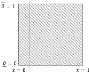
Consumers are uniformly distributed over a rectangular space of characteristics.

Characteristics are each consumer’s location (𝑥) in the unit interval (𝑥 ∈ [0; 1]) and 𝜃, 𝜃

representing the valuation of quality. While in the previous setting consumers were

assumed to have equal tastes for quality (𝜃 = 1), here tastes vary across individuals. Such

as in similar applications – Economides (1989) – we normalize 𝜃 without loss of generality

so that 𝜃 ϵ [0; 1]. Consumers are thus uniformly distributed over the unit square 𝑍 =

[0; 1] × [0; 1]. The product space is defined by the quality characteristic delimited by the

qualities of the lower quality and higher quality fuels (𝑠, 𝑠 𝜖 [𝑠𝐿, 𝑠𝐻]). Firms’ quality

choices are not continuous as they can only choose between the lower (𝑠𝐿) and higher

quality fuels (𝑠𝐻) being therefore restrained from choosing any level of quality in between.

Figure 1 - Consumers uniformly distribution over the characteristics space

This setting encompasses both 2-dimensions differentiation and varying tastes for quality.

For each location x, consumers located in the same vertical line (see figure 1) have

(9)

3.3. Heterogeneous non-continuous tastes and three qualities

Although firms’ choice is between premium and regular fuels, the obligation to supply low

-quality fuel certainly influences firm’s decisions. Hence there is interest in examining a

three-qualities market setting. An ideal exercise would accommodate continuous and

heterogeneous preferences for quality in the existence of three qualities. The presence of an

equilibrium would be analyzed as usual in order to assess the possible outcomes of the

game. Such exercise entails a complex system of equation mainly as a consequence of

non-linear demands, limiting the scope for useful results and implications.

The following model is, without loss of generality, a simplified alternative that considers a

concentration of consumers along three different Hoteling lines, each corresponding to

different levels of taste for quality 𝜃𝐿, 𝜃𝑀and 𝜃𝐻 (with 𝜃𝑙< 𝜃𝑚 < 𝜃ℎ). Each line has

length 1 and a mass of 1/3 consumers uniformly distributed over it, ensuring that the total

mass of consumers is 1, as in the previous exercises. Although the taste for quality is not

continuous, this ensures a certain degree of heterogeneity in consumers’ tastes for quality.

The individual consumer utility is given by

𝑣 + 𝜃𝑠𝑖 − 𝑝 − 𝑡(𝑑𝑖𝑠𝑡𝑎𝑛𝑐𝑒) (1)

Fuels’ quality levels are defined a priori, and assumed to be represented by 𝑠𝐿 = 0, 𝑠𝑀 =1 2

and 𝑠𝐿 = 1. Marginal costs of production are quality specific across firms, respecting the

(10)

4 Strategies, Equilibria and Implications

In the following models we use backward induction to search for the existence of a

subgame perfect equilibrium. Firms first compete in qualities and then prices. By

performing the usual profit maximization exercise – after identifying consumers’

indifference relations and demands for each product – equilibrium prices are obtained.

Finally demands and profits resulting from equilibrium prices are found. For each model a

table of payoffs displays firms’ profits for each outcome. Analysis will focus on the

existence or not of subgame perfect Nash equilibria in quality, on the different conditions

for each equilibrium market configuration and on the conditions dictating asymmetric

quality choices being or not an equilibrium.

4.1. Homogeneous consumers and two qualities

The indifferent consumer is located at x where its utility of buying from firm 1 is equal to

that achieved by buying from firm 2, respecting:

𝑣 + 𝑠1− 𝑝1− 𝑡(𝑥) = 𝑣 + 𝑠2− 𝑝2− 𝑡(1 − 𝑥) (2)

Hence the indifferent consumer is located at:

𝑥 =𝑠1− 𝑠2+ 𝑝_2𝑡2− 𝑝1+ 𝑡 (3)

Note that because x is increasing in 𝑠₁and decreasing in 𝑠₂ it is clear that the higher firm’s 1

quality is compared to 2’s, the higher will be its market. Because all consumers located in

(11)

demand for firm 1 (_{1 − 𝐷}₁_{= 𝐷}₂). To ensure that a firm is never priced out of the market the

following condition has to be respected

∆𝑠𝑖 − ∆𝑃𝑖

3𝑡 < 0,5 (4)

From this point each firm can find its profit maximizing prices (or response function) (xxx)

and, by incorporating the other firm’s response function, equilibrium prices can be found,

depending on the qualities, transportation costs and production costs of the different

products (note that different qualities have different constant marginal costs of production.

Firm i’s price at equilibrium will be:

𝑝𝑖∗ =𝑠𝑖 − 𝑠𝑗+ 3𝑡 + 2𝑐₃ 𝑖+ 𝑐𝑗 (5)

With the second stage equilibrium prices firms’ profits at equilibrium can be easily

determined, as a function of all marginal costs, qualities and transportation costs – please

see equation (8) further in this section. Regarding the choice of quality three situations can

happen:

1. Both firms choose to offer the premium (high quality) fuel;

2. One firm decides to offer the premium (high quality) fuel while the other chooses to

offer the regular (lower quality) fuel;

3. Both firms choose to offer the regular (low quality) fuel.

Note that in the cases 1 and 3, where both firms offer the same quality, this exercise boils to

a standard Hotelling line situation – with differentiation happening only in the horizontal

(12)

competition dictates equal split of demand and profits between firms and the indifferent

consumer has its location in the middle of the unit segment. Equilibrium prices are then

equal across firms corresponding to the Hotelling model, yielding:

𝑝∗ _{= 𝑝}

1 = 𝑝2 = 𝑡 + 𝑐 (6)

However, when situation 2 occurs differentiation is both in quality and location. Being the

qualities chosen different prices will also be distinct. The difference in the equilibrium

prices is given by:

2∆𝑠𝑖+ ∆𝑐𝑖

3 (7)

with ∆𝑠_𝑖= 𝑠_𝑖− 𝑠_𝑗𝑎𝑛𝑑 ∆𝑐_𝑖= 𝑐_𝑖− 𝑐_𝑗, 𝑗, 𝑠 = 1,2, 𝑗 ≠ 𝑠

Making the assumption |∆𝑠_𝑖| > |∆𝑐_𝑖| it is an immediate result a higher price for the higher

quality product and a lower price for the lower quality, when comparing to the prices that

would emerge as an equilibrium in case of a market outcome of only one type of fuel being

offered. Whatever the case, taking equilibrium prices and subsequent demand for those

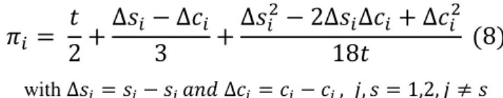
prices into consideration, profits in equilibrium are determined by:

𝜋𝑖 = _{2 +}𝑡 ∆𝑠𝑖 − ∆𝑐₃ 𝑖+∆𝑠𝑖

2_{− 2∆𝑠}

𝑖∆𝑐𝑖 + ∆𝑐𝑖2

18𝑡 (8)

Note that, as indicated, situations 1 and 2 correspond symmetric demand and hence profits

in equilibrium, being the former equal to

𝜋1 = 𝜋2 =_{2 (9)}𝑡

(13)

Firms’ choices FIRM 2

Low Quality _{High Quality}

FIRM 1

Low Quality (𝑡

2; 𝑡

2 ) ( 2𝑡+ ∆𝜋1 𝐿

; ₂𝑡+ ∆𝜋₂𝐻 )

High Quality ( 𝑡

2+ ∆𝜋1 𝐻

; ₂𝑡+ ∆𝜋₂𝐿 ) ( 𝑡

2; 𝑡 2 )

Given one firm’s quality, the other firm’s profit difference between choosing the same or a

different quality is given by the difference between (5) and (6):

∆𝜋𝑖 = ∆𝑠𝑖− ∆𝑐₃ 𝑖+(∆𝑠𝑖− ∆𝑐𝑖) 2

18𝑡 (10)

∆𝜋 = ∆𝜋𝑖𝐻 𝑖𝑓 𝑓𝑖𝑟𝑚 𝑖 𝑐ℎ𝑜𝑜𝑠𝑒𝑠 𝑡𝑜 𝑜𝑓𝑓𝑒𝑟 𝑡ℎ𝑒 ℎ𝑖𝑔ℎ𝑒𝑟 𝑞𝑢𝑎𝑙𝑖𝑡𝑦 𝑎𝑛𝑑 𝑓𝑖𝑟𝑚 𝑗 𝑡ℎ𝑒 𝑙𝑜𝑤𝑒𝑟 𝑜𝑛𝑒

∆𝜋 = ∆𝜋𝑖𝐿 𝑖𝑓 𝑓𝑖𝑟𝑚 𝑖 𝑐ℎ𝑜𝑜𝑠𝑒𝑠 𝑡𝑜 𝑜𝑓𝑓𝑒𝑟 𝑡ℎ𝑒 𝑙𝑜𝑤𝑒𝑟 𝑞𝑢𝑎𝑙𝑖𝑡𝑦 𝑎𝑛𝑑 𝑓𝑖𝑟𝑚 𝑗 𝑡ℎ𝑒 ℎ𝑖𝑔ℎ𝑒𝑟 𝑜𝑛𝑒

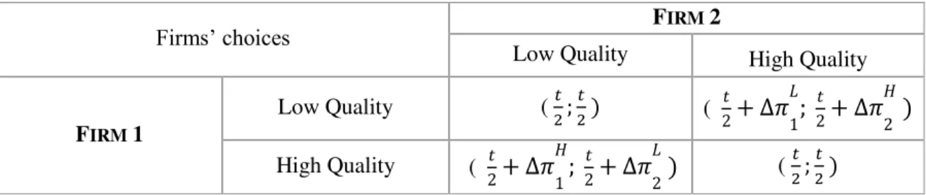
Table 1 provides information on the profits each firms obtains in the different outcomes.

Note that from (10) it is clear that both ∆𝜋_𝑖𝐻and ∆𝜋_𝑖𝐿 are always positive. A direct

implication is that the pairs (low; high) and (high; low) are subgame perfect Nash equilibria

in pure strategies for quality choices - no firm has an incentive to unilaterally move away

from that outcome. If a firm chooses “low” than the other firm would prefer to choose

“high”, whereas if a firm chooses to play “high” than the other would find it more

profitable to play “low”. The pairs (low; low) and (high; high) are never subgame perfect

Nash equilibria, as both firms have incentives to deviate from such outcomes.

Regarding the magnitude of the differences in profits from breaking from a (high; high) or

(low; low) qualities equilibrium, the higher the difference in quality comparing to that of

marginal costs – see equation (11) below –the bigger profits’ difference is. If it comes to a

(14)

exactly equals the increase in quality, then no benefits are created form the form by

changing the quality offered. The costs increase effect equals the quality increase effect

leaving the profits unchanged.

lim

∆𝑐𝑖→∆𝑠𝑖∆𝜋𝑖 = 0 (11)

4.2. Heterogeneous consumers and two qualities

The indifferent consumer is that in such location that the following equality occurs:

𝑣 + 𝜃𝑠1− 𝑝1 − 𝑡(𝑥) = 𝑣 + 𝜃𝑠2− 𝑝2− 𝑡(1 − 𝑥) (12)

Rewriting the expression, one obtains firm 1’s market share for type 𝜃:

𝑥(𝜃) =𝜃(𝑠1− 𝑠2) + 𝑝2− 𝑝1+ 𝑡

2𝑡 (13)

Integrating (11) from 0 to 1 in 𝜃the expression for firm 1’s total demand is found:

∫ 𝑥(𝜃)𝜃

𝜃 = ∫ 𝑥(𝜃)

1

0 = 𝐷𝑖 =

1 2 +

𝑠1− 𝑠2+ 2(𝑝𝑗− 𝑝𝑖)

4𝑡 (14)

From which the following condition is withdrawn to ensure that no firm is priced out of the

market by the other firm:

𝑠1− 𝑠2+ 2(𝑝𝑗− 𝑝𝑖)

4𝑡 < 0,5 (15)

Employing the computed expressions for demand and performing the profits maximization

in respect to own prices, profit-maximizing prices for each firm – response functions – are

(15)

𝑝_𝑖∗ _{= 𝑡 +}2𝑐𝑖+ 𝑐𝑗

3 +

𝑠𝑖− 𝑠𝑗 6 (16)

It immediately follows that whenever firms choose to offer the same quality, prices will be

the same. If firms’ choice leads to quality differentiation, then the high quality fuel will also

have a higher price – the higher the cost and quality gaps between the two qualities the

higher the price difference – comparing to the low quality one.

It is also interesting to analyze the effect of differentiation on the prices of the different

products having as baseline the situation where the market offers only one quality. Whether

the price of the high quality fuel offered by one firm (when the other firm offers the

alternative quality) is higher or lower than the equilibrium price of that same quality when

both firms offer it depends on the relations between cost and quality levels’ difference. The

same inference is valid for the case of the low quality fuel.

𝑃_𝑖𝐻(𝐻)− 𝑃_𝑖𝐻(𝐿)= 𝑃_𝑖𝐿(𝐻)− 𝑃_𝑖𝐿(𝐿) =2(𝑐𝐻₆− 𝑐𝐿)+(𝑠𝐿− 𝑠₆ 𝐻)(17)

Note that the last term of the equation is always negative, while the penultimate is always

positive. The resulting impact arises from the difference relation of these terms. If

2(𝑐𝐻−𝑐𝐿) 6 >

(𝑠𝐿−𝑠𝐻)

6 low cost product price is higher when firms differentiate and the high

quality fuel’s price is higher when both firms offer that quality. If 2(𝑐𝐻−𝑐𝐿) 6 <

(𝑠𝐿−𝑠𝐻) 6 the

opposite occurs. Incorporating equilibrium prices in the profits function, profits in

equilibrium are derived and given by:

𝜋𝑖 = _{2 +}𝑡 7∆𝑠_{12 −}𝑖 ∆𝑐_{2 +}𝑖 ∆𝑠𝑖 2 12𝑡 +

∆𝑐𝑖2 9𝑡 −

(16)

As in the previous model, when firms do not differentiate themselves in the quality

dimension, their profits in equilibrium are the same regardless of the quality offered. The

exercise comes down to a Hotelling outcome. To find a hypothetical equilibrium it is

essential to look at the possible payoff pairs resulting from the game:

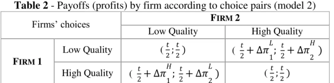
Table 2 - Payoffs (profits) by firm according to choice pairs (model 2)

Low Quality High Quality

FIRM 1

Low Quality (𝑡

2; 𝑡

2 ) ( 2𝑡+ ∆𝜋1 𝐿

; ₂𝑡+ ∆𝜋₂𝐻 )

High Quality ( ₂𝑡+ ∆𝜋

1 𝐻

; ₂𝑡+ ∆𝜋₂𝐿 ) ( 𝑡

2; 𝑡 2 )

Again, for simplicity of the analysis, considering the possibility of isolated modes from a first set of choices,∆𝜋_𝑖 represents the difference in profits one firm would face by moving

from a situation where they offer the same quality, assuming that the other firm does not

change its own quality.

∆𝜋𝑖 = +7∆𝑠𝑖₁₂− 6∆𝑐𝑖+3∆𝑠𝑖

2_{+ 4∆𝑐}

𝑖2− 8∆𝑠𝑖∆𝑐𝑖

36𝑡 (19)

∆𝜋 = ∆𝜋𝑖𝐻 𝑖𝑓 𝑓𝑖𝑟𝑚 𝑖 𝑐ℎ𝑜𝑜𝑠𝑒𝑠 𝑡𝑜 𝑜𝑓𝑓𝑒𝑟 𝑡ℎ𝑒 ℎ𝑖𝑔ℎ𝑒𝑟 𝑞𝑢𝑎𝑙𝑖𝑡𝑦 𝑎𝑛𝑑 𝑓𝑖𝑟𝑚 𝑗 𝑡ℎ𝑒 𝑙𝑜𝑤𝑒𝑟 𝑜𝑛𝑒

∆𝜋 = ∆𝜋𝑖𝐿 𝑖𝑓 𝑓𝑖𝑟𝑚 𝑖 𝑐ℎ𝑜𝑜𝑠𝑒𝑠 𝑡𝑜 𝑜𝑓𝑓𝑒𝑟 𝑡ℎ𝑒 𝑙𝑜𝑤𝑒𝑟 𝑞𝑢𝑎𝑙𝑖𝑡𝑦 𝑎𝑛𝑑 𝑓𝑖𝑟𝑚 𝑗 𝑡ℎ𝑒 ℎ𝑖𝑔ℎ𝑒𝑟 𝑜𝑛𝑒

From (19) it immediately follows that while ∆𝜋_𝑖𝐻 can be either positive or negative, ∆𝜋_𝑖𝐿 is

always negative. There are thus two variations: when ∆𝜋_𝑖𝐻 is positive and ∆𝜋_𝑖𝐿 negative;

when ∆𝜋_𝑖𝐻 is negative and ∆𝜋_𝑖𝐿 also negative. In the first case firms have an equilibrium in

dominant strategies choosing to play “high” – leading to the outcome (high; high). That

(17)

yields lower profits for the firm changing strategy and even allows the competitor to

increase profits without having to change its strategy. When both elements are negative,

situation to which, ceteris paribus, eventual increases in the transportation costs parameter t

contribute, then firms have a symmetric Nash equilibria in pure strategies in choosing not

to differentiate in qualities –that is, both playing “high” or both playing “low”. Whatever

the case, subgame perfect Nash equilibria is only present in scenarios where no vertical

differentiation occurs It is also interesting to note that the more “sensitive” consumers are

to the horizontal dimension the more likely are firms not to differentiate in the vertical

dimension.

lim

∆𝑐𝑖→∆𝑠𝑖∆𝜋𝑖 =

3∆𝑠𝑖 36 −

∆𝑠𝑖2 36𝑡

𝑦𝑖𝑒𝑙𝑑𝑠

→ { ∆𝜋_∆𝜋 𝑖 > 0, 𝑓𝑜𝑟 ∆𝑠𝑖 ∈ [0; 1] 𝑖 < 0, 𝑓𝑜𝑟 ∆𝑠𝑖 ∈ [−1; 0] (20)

Computations in (20) also present useful aspects. For a situation where both

|∆𝑠𝑖|and|∆𝑐𝑖| ∈ [0; 1], ∆𝜋𝑖 is always positive when a firm offers the high quality fuel

whereas the opposite occurs when the low quality fuel is the firm’s choice.14 In this setting

outcome (high; high) is a subgame perfect Nash equilibrium in dominant strategies.15

4.3. Heterogeneous non-continuous tastes and three qualities

Initial analysis focuses on the situation where both firms offer the low-quality fuel, and

then differentiate themselves in the remaining qualities (firm 1 offers the high-quality fuel

and firm 2 offers the medium-quality fuel – this specific choice is irrelevant due to the

symmetry of results in an opposite case). In order to perform the profits maximization that

14

Consider the normalization𝑡 = 1 .

15

(18)

allow for the search of equilibrium prices, demands are obtained from the indifference

relations present in this framework. It is assumed that consumers consume the quality

“closer” to their tastes, meaning that whenever the market offers all qualities, consumers

with lower taste for quality (𝜃𝑙) will only choose between low and medium qualities while

consumers with higher taste for quality (𝜃ℎ) would choose only between high and medium

qualities.

Indifference relations:

 For 𝜃ℎ consumers, between high and medium quality fuels (21);

 For 𝜃𝑚consumers, between high and medium quality fuels (22); and between

medium quality and low quality (supplied by firm 1) fuels (23)

 For 𝜃𝑙 consumers, between medium quality and low quality (supplied by firm 1)

fuels (24); and between low quality fuels supplied by the two firms (25)

𝑥 =𝑝2𝑀−𝑝1𝐻 2𝑡 +

1 2+

𝜃ℎ

4𝑡 (21) 𝑥 =

𝑝2𝑀−𝑝1𝐻 2𝑡 +

1 2+

𝜃𝑚 4𝑡 (22)

𝑥 =𝑝2𝑀−𝑝1𝐿 2𝑡 +

1 2−

𝜃𝑚

4𝑡 (23) 𝑥 =

𝑝₂𝑀−𝑝₁𝐿 2𝑡 +

1 2−

𝜃𝑙

4𝑡 (24) 𝑥 = 𝑝₂𝐿−𝑝₁𝐿

2𝑡 + 1

2 (25)

Figure 2–Firms’ and Consumers’ space of characteristics illustration

Observing figure 2 the location of each of the indifferent consumers’ position entails

relevant underlying assumptions. If, as depicted, (25) < (24) and (22) < (23) this is

equivalent to 𝑝₂𝑀− 𝑝₁𝐿 > 𝜃𝑙

(19)

the high quality fuel over the low-quality fuel provided by firm 1; and no 𝜃𝑙consumer

prefers the medium quality fuel over the low quality fuel supplied by firm 2, as the

increase in utility is not enough to compensate the higher price. In an opposite case, that is

𝑝2𝑀− 𝑝1𝐿 < 𝜃 𝑙

2 and 𝑝1𝐻− 𝑝1𝐿 < 𝜃𝑚 there would be no demand for firm 1’s low quality fuel.

Hence, aggregated demands for each product yield:

𝐷1𝐻= 1₆+𝑝2 𝑀_−𝑝

1 𝐿 2𝑡

𝜃ℎ

4𝑡 (26) 𝐷1𝐿 =

2 6+

𝑝₂𝑀+𝑝₁𝐿−2𝑝₁𝐿 2𝑡

𝜃ℎ 4𝑡 (27)

𝐷2𝑀 =2₆+𝑝1 𝐻_−𝑝

1 𝐿_−2𝑝

2 𝑀

2𝑡 +

𝜃𝑚_−𝜃ℎ

4𝑡 (28) 𝐷2𝐿 = 1 6+

𝑝1𝐿−𝑝2𝐿 2𝑡 (29)

With demands, profits – at an aggregated level for each firm, that is, considering for each

firm the costs, prices and demand associated with each specific product they offer – can be

easily computed, allowing for the profit maximization exercise, in order to find equilibrium

prices. Equilibrium prices found lead to specific demands (at equilibrium) and consequently

profits. To test this market setting – where firms differentiate themselves in the

quality-choice available, given that both are required to offer the low quality fuel, these profits

have to be compared to those arising from the other possible market configurations: both

firms offering the low-quality and the medium quality fuels; or both firms offering the low

quality and high quality fuels. In both these cases the exercise is simplified to a classical

Hotelling. Regardless the assumptions – regarding consumers’ preferring always one

quality to another – in equilibrium firms will equally divide the market and earn profits:

(20)

Firms, by anticipating the possible outcomes of the game, will ultimately choose the

strategy that leads to higher payoffs (profits). The following table shows the profits

emerging for each of the firms according to the possible strategies. Although not

specifically identified these are the aggregate profits – that is, also considering those arising

from supplying the low-quality fuel – as the setting

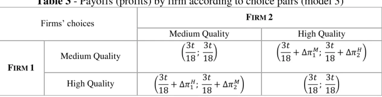
Table 3 - Payoffs (profits) by firm according to choice pairs (model 3)

Medium Quality High Quality

FIRM 1

Medium Quality (

3𝑡 18 ;

3𝑡

18) (

3𝑡

18 + ∆𝜋1𝑀; 3𝑡

18 + ∆𝜋2𝐻)

High Quality (3𝑡

18 + ∆𝜋1𝐻; _{18 + ∆𝜋}3𝑡 2𝑀) (_{18 ;}3𝑡 ₁₈₎3𝑡

∆𝜋𝑖𝐻: 𝑖𝑓 𝑓𝑖𝑟𝑚 𝑖 𝑐ℎ𝑜𝑜𝑠𝑒𝑠 𝑡𝑜 𝑜𝑓𝑓𝑒𝑟 𝑡ℎ𝑒 ℎ𝑖𝑔ℎ𝑒𝑟 𝑞𝑢𝑎𝑙𝑖𝑡𝑦 𝑎𝑛𝑑 𝑓𝑖𝑟𝑚 𝑗 𝑡ℎ𝑒 𝑚𝑒𝑑𝑖𝑢𝑚 𝑜𝑛𝑒

∆𝜋𝑖𝑀: 𝑖𝑓 𝑓𝑖𝑟𝑚 𝑖 𝑐ℎ𝑜𝑜𝑠𝑒𝑠 𝑡𝑜 𝑜𝑓𝑓𝑒𝑟 𝑡ℎ𝑒 𝑚𝑒𝑑𝑖𝑢𝑚 𝑞𝑢𝑎𝑙𝑖𝑡𝑦 𝑎𝑛𝑑 𝑓𝑖𝑟𝑚 𝑗 𝑡ℎ𝑒 ℎ𝑖𝑔ℎ𝑒𝑟 𝑜𝑛𝑒

Again, ∆𝜋_𝑖 represents the difference in the total profits one firm would face by moving

from a situation where the two firms offer the same quality, assuming that the other does

not change its own quality. Please see elements ∆𝜋_𝑖𝐻 and ∆𝜋_𝑖𝑀 in appendix (A.12) and

(A.13) respectively. Strategies are choosing either medium or high quality. Assessing

possible equilibria depends not only on the differences of costs and qualities but also on the

transportation costs (t). If both ∆𝜋_𝑖𝐻 and ∆𝜋_𝑖𝐿are negative, then pairs (high; high) and (low;

low) are symmetric Nash equilibria in pure strategies – any deviation ∆𝜋_𝑖 would decrease

the deviant’s profits therefore firms will choose to minimal quality differentiation. By

contrast, if ∆𝜋_𝑖𝐻 and ∆𝜋_𝑖𝐿 are both positive then the pairs (high; low) and (low; high) are

asymmetric subgame perfect Nash equilibria in pure strategies. In a different situation,

(21)

lower profits then firms will both – see the symmetric properties (32) – have a weekly

dominant strategy in choosing to offer the quality to which a deviation from a

same-qualities pair results in higher profits. The resulting outcome will be the pair of same

strategies (resulting in minimal vertical differentiation) from which no firm will have

incentives to unilaterally move away from and therefore, a subgame perfect Nash

equilibrium in dominant strategies.

These results, although limited in terms of interpretation, shed a light on how empty can

policymakers’ arguments be when firms-level information is opaque or not available to the

public and governments. Further exploring the possibilities of this model one can look at

the welfare implications of mandatory low quality fuel provision. Since fully covered

market is being assumed one can search for the welfare distribution for the agents in the

market. That assumption is maintained for consistency’s sake. Although recognized that a

welfare analysis under different conditions could also provide interesting results, it should

follow configurations that account for non-fully covered markets. Given that all consumers

buy fuel (whatever the quality or provider) prices provide all information about their

welfare in market configurations where firms offer the same qualities. In a situation where

only medium and high quality are offered consumers would pay a total of 𝑡 +2𝑐𝑀+𝑐𝐻 3 .

Comparing with the cases where: both firms offer the low-cost and medium qualities; and

that where both firms offer medium and low quality; a market situation where no low-cost

is offered and both firms supply the remaining qualities yields lower aggregate consumers’

(22)

situation where firms decide to differentiate themselves direction of the effect on

consumers’ expenditure cannot be identified beforehand. It depends on the magnitude of

the differences between costs and also on the differences between the tastes for quality of

heterogeneous consumers. In the scope of this model without clear information about the

preferences’ and costs’ parameters policymakers would not have the ability to anticipate

consumers’ welfare variation.

5 Conclusion

This work aimed at exploring the challenges faced by fuel retailer firms as a result of

legislation imposing mandatory supply of low quality fuel, and understanding the market

implications of such measure. It has particularly focused on firms’ strategic behavior under

capacity constraints and two-dimensional product differentiation.

Results suggest that under no consumers’ heterogeneity firms have two asymmetric Nash

equilibria in choosing to differentiate over the quality dimension, both earning positive and

higher profits than comparing with the no-differentiation alternative. However, when

consumer heterogeneity is maximal (and continuous), vertical differentiation is not a

subgame perfect Nash equilibrium. Instead, either in pure strategies or weekly dominating

strategies, firms have a subgame perfect Nash equilibrium in opting for minimum quality

differentiation. When no equilibria exist in pure strategies exists firms have a weekly

dominating equilibrium in choosing to offer only high quality fuel. When considering a

three-qualities setting firms’ preferable strategies can not be identified a priori. Consistent

(23)

magnitude of the incentives firms may have to differentiate Differentiation can lead to both

qualities being available at either higher or lower prices. Introduction of mandatory “low

cost” fuels does not guarantee per si higher welfare to consumers. In fact, consumers can be

jeopardized with such measure. If both firms offer exactly the same qualities consumers’

expenditure is higher than that verified when both firms offer medium and high qualities

simultaneously. If firms choose to differentiate over the non-mandatory qualities the effect

of consumers’ welfare is not clear, depending on the costs hiatus and level of consumer

heterogeneity. After being required to offer “low-cost” fuel Portuguese retail firms chose a

certain level of vertical differentiation as no quality was eliminated from the market.16

Under duopoly and assumed maximal differentiation on the horizontal dimension there is

no evidence supporting with certainty (without knowing firms’ costs and consumers’

preferences and perceptions) the maximal differentiation on both dimensions is a stable

equilibrium, but neither is evidence excluding the possibility.

This is merely a theoretical approach but the novelty of the policy studied demands further

study. Empirical works could be developed with more transparent data allowing authors to

test the robustness of theoretical models.17 Even without such data there is room for

extending this work into considering settings comprising more firms in the market, search

costs for consumers’, heterogeneous perceptions of quality and the ties between retail and

higher levels on the vertical value chain of the fuels’ market.

16

Repsol, Cepsa and BP eliminated the medium quality fuel while Galp eliminated the premium quality fuel.

17

(24)

References

Borenstein, Severin. et al.. 1997. “Do gasoline prices respond asymmetrically to crude oil price changes?”

The Quarterly Journal of Economics, vol. 112(1); 305–339.

Borenstein, Severin. and Shepard, Andrea. 1996. “Dynamic pricing in retail gasoline markets.” RAND Journal of Economics, vol. 27(3): 429–451.

Bacon, Robert.1991. “Rockets and feathers: the asymmetric speed of adjustment of UK retail gasoline prices to cost changes.”Energy Economics, 13(3): 211–218.

Clark, Robert; Houde, Jean-François. 2013. “Collusion with Asymmetric Retailers: Evidence from a Gasoline Price-Fixing Case.”American Economic Journal, 5(3): 97-123.

d'Aspremont, Château. et al.1979. “On Hotelling's "stability in Competition.” Econometrica, 47(5): 1145– 1150.

Degryse, H.1996. “On the Interaction Between Vertical and Horizontal Product Differentiation: An

Application to Banking.” The Journal of Industrial Economics, 44(2): 169–186.

Edgeworth, Francis. 1925. “The Pure Theory of Monopoly.” Papers Relating to Political Economy, 1: 111-142.

Godby, Robert. et al.. 2000. “Testing for asymmetric pricing in the Canadian retail gasoline market.”Energy Economics, 22(3): 349–368.

Irmen, Andreas. and Thisse, Jacques. 1998. “Competition in Multi-characteristics Spaces: Hotelling Was Almost Right.” Journal of Economic Theory, 78: 76-102.

Jhnson, Ronald. 2002. “Search costs, lags and prices at the pump.”Review of Industrial Organization, 20(1): 33–50.

Maskin, Eric. and Tirole, Jean. 1988. “A theory of dynamic oligopoly, II: price competition, kinked demand curves, and Edgeworth cycles.”Econometrica, 56: 579–599.

Netz, Janet S. and Taylor, Beck.2002. “Maximum or Minimum Differentiation? Location Patterns of Retail

Outlets.”Review of Economics and Statistics, 84(1): 162-175.

Neven, Damien. 1985. “Two Stage (Perfect) Equilibrium in Hotelling's Model.” The Journal of Industrial Economics, 33(3): 317-325.

Neven, Damien. and Thisse, Jacques François.1987. “Combining Horizontal and Vertical Differentiation:

The Principle of Max-min Differentiation.” INSEAD Working Papers.

Saked, Avner. and Sutton, John.1982. “Relaxing Price Competition Through Product Differentiation.” The Review of Economic Studies, 49(1): 3–13.

Salop, Steven. 1979, “Monopolistic Competition with Outside Goods.” Bell Journal of Economics, 10(1): 141-156.

Tabuchi, Takatoshi.1994, “Two-stage two-dimensional spatial competition between two firms.” Regional Science and Urban Economics, 24(2): 207–227.

Wang, Zhongmin.2008. “Collusive Communication and Pricing Coordination in a Retail Gasoline Market.”

(25)

Appendix

A.1 Model 1

𝐷𝑖(𝑝𝑖∗,𝑝𝑗∗)= 1₂+∆𝑠𝑖_6𝑡−∆𝑐𝑖 (A-1); 𝜋𝑖 = ₂𝑡+∆𝑠𝑖−∆𝑐₃ 𝑖+∆𝑠𝑖 2_−2∆𝑠

𝑖∆𝑐𝑖+∆𝑐𝑖2

18𝑡 (A-2)

A.2 Model 3

If, besides the low cost fuel a firm decides to offer medium quality and the other firm high quality

𝑝_𝑖𝐻 ₌𝑡 3+

5𝑐𝐿_+14𝑐𝑀_+26𝑐𝐻

45 +

5𝜃𝑚_+19𝜃ℎ

90 (A-4); 𝐷𝑖𝐻 16+

5𝑐𝐿_+14𝑐𝑀_−19𝑐𝐻

90𝑡 +

180𝑡 (A-8)

𝑝𝑗𝑀=₃𝑡+10𝑐

𝐿_+28𝑐𝑀_+7𝑐𝐻

45 +

10𝜃𝑚−7𝜃ℎ

90 (A-5); 𝐷𝑗𝑀= 1 3+

20𝑐𝐿−34𝑐𝑀+14𝑐𝐻

90𝑡 +

20𝜃𝑚−13𝜃ℎ 180𝑡 (A-9)

𝑝𝑖𝐿=₃𝑡+2𝑐

𝐻_+8𝑐𝑀_+35𝑐𝐿

45 −

10𝜃𝑚_+𝜃ℎ

90 (A.6); 𝐷𝑖𝐿= 1 3+

4𝑐𝐻_+57𝑐𝑀_−20𝑐𝐿

90𝑡 −

360𝑡 (A.10)

𝑝_𝑗𝐿₌ 𝑡 3+

𝑐𝐻_+4𝑐𝑀_+40𝑐𝐿

45 −

10𝜃𝑚_+𝜃ℎ

180 (A.7); 𝐷𝑗𝐿 16+

𝑐𝐻_+4𝑐𝑀_−5𝑐𝐿

90𝑡 (A.11)

∆𝜋𝑖𝐻 =(𝜋1𝐿+ 𝜋1𝐻) −₁₈3 𝑡 (A.12) ∆𝜋𝑖𝑀=(𝜋2𝐿+ 𝜋2𝑀) −₁₈3 𝑡 (A.13)

∆𝜋_𝑖𝐻_{− ∆𝜋}

𝑖𝑀= (𝜋1𝐿− 𝜋2𝐿) + (𝜋1𝐻− 𝜋2𝑀) (A.14)

𝜋1𝐿 = [(𝑡₃+2𝑐

𝐻_+8𝑐𝑀_−10𝑐𝐿

45 −

10𝜃𝑚_+𝜃ℎ 90 ) (

1 3+

4𝑐𝐻_+57𝑐𝑀_−20𝑐𝐿

90𝑡 −

360𝑡 )] (A.15)

𝜋1𝐻 _{= [(}𝑡 3+

45 +

5𝜃𝑚_+19𝜃ℎ 90 ) (

1 6+

90𝑡 +

180𝑡 )] (A.16)

𝜋2𝐿 = [(𝑡₃+𝑐

𝐻_+4𝑐𝑀_−5𝑐𝐿

45 −

10𝜃𝑚_+𝜃ℎ 180 ) (

1 6+

𝑐𝐻_+4𝑐𝑀_−5𝑐𝐿

90𝑡 )] (A.17)

𝜋2𝑀= [(𝑡₃+10𝑐

𝐿_−17𝑐𝑀_+7𝑐𝐻

45 +

10𝜃𝑚_−7𝜃ℎ 90 ) (

1 3+

20𝑐𝐿_−34𝑐𝑀_+14𝑐𝐻

90𝑡 +

20𝜃𝑚_−13𝜃ℎ