A Novel Ensemble Method for Regression via Classification Problems

(1)

ISSN 1549-3636

Corresponding Author: Sami M. Halawani, Department of Information Technology, Faculty of Computing and Information Technology, King Abdul Aziz University, Rabigh, Saudi Arabia Tel: 00966533515050 Fax-0096622434030

A Novel Ensemble Method for Regression via Classification Problems

1

Sami M. Halawani, 2Ibrahim A. Albidewi and 1Amir Ahmad 1

Department of Information Technology, Faculty of Computing and Information Technology,

King Abdul Aziz University, Rabigh, Saudi Arabia 2_{Department of Information Systems,}

Faculty of Computing and Information Technology, King Abdul Aziz University, Jeddah, Saudi Arabia

Abstract: Problem statement: Regression via Classification (RvC) is a method in which a regression

problem is converted into a classification problem. A discretization process is used to covert continuous target value to classes. The discretized data can be used with classifiers as a classification problem. Approach: In this study, we use a discretization method, Extreme Randomized Discretization (ERD), in which bin boundaries are created randomly to create ensembles. Results: We show that the proposed ensemble method is useful for RvC problems. We show theoretically that the proposed ensembles for RvC perform better than RvC with the equal-width discretization method. We also show the superiority of the proposed ensemble method experimentally. Experimental results suggest that the proposed ensembles perform competitively to the method developed specifically for regression problems. Conclusion: As the proposed method is independent of the choice of the classifier, various classifiers can be used with the proposed method to solve the regression method.

Key words: Regression via Classification (RvC), ERD ensembles, classification problem, decision

trees, Extreme Randomized Discretization (ERD), Monothetic Contrast Criteria (MCC), RvC perform, Mean Square Error (MSE), neural network

INTRODUCTION

In machine learning and data mining fields, supervised learning plays an important role (Bishop 2006; Mitchell, 1997; Halawani and Albidewi, 2010; Ahmad and Dey, 2005; Ahmad and Brown, 2009; Chandra et al., 2010; Alfred, 2010; Ishrat et al., 2010). In a regression problem, the target values are continuous, whereas in the classification problem we have discrete set of classes. The other difference is that regression values have a natural ordering, whereas for the classification the class values are unordered (Bishop, 2006; Mitchell, 1997). Regression models are not easily understood by domain experts and thus provide little help in understanding the problem, whereas classification models are more comprehensible, but not very useful, when the target values are continuous. There are some learning schemes, like naive Bayes, which are very successful as classification techniques, however, they are difficult to use as regression schemes. Decision trees (Breiman et al., 1984; Quinlan, 1993), neural networks (Bishop, 2006; Mitchell, 1997), naive Bayes (Bishop, 2006;

Mitchell, 1997), support vector machines (Vapnik, 1998; Burges, 1998) are quite popular for classification problems, whereas regression trees (Breiman et al., 1984), neural networks (Bishop, 2006; Mitchell, 1997), support vector machines (Vapnik, 1998; Burges, 1998) are used for regression problems.

(2)

388 (MCC) (Merckt, 1993) are unsupervised methods. Discretization methods based on entropy (supervised MCC (Merckt, 1993) and Vector Quantization (Kohonen, 1989) are supervised methods. Equal-width intervals and equal-frequency intervals are global methods. The discretization used in the C4.5 decision tree growing phase and Vector Quantization are local methods. All these methods are static methods. Dynamic methods are a promising area of research. As these methods are able to capture interdependencies between attributes, it may improve the accuracy of decision rules.

Researchers (Torgo and Gama, 1996; 1997a; 1997b; Indurkhya and Weiss, 2001) suggest that the discretitaion process can be used to convert continuous target values into a discrete set of classes and then classification models are used to solve the classification problems. In other words, in a RvC problem, a regression problem is solved by converting into a classification problem. This method employs any classifier on a copy of the data that has the target attribute discretized. The whole process of RvC comprises two important stages:

• The discretization of the numeric target variable in order to learn a classification model. There are different discretzation methods e.g., equal-width, equal-frequency (Dougherty et al., 1995)

• The reverse process of transforming the class output of the classification model into a numeric prediction. We may use the mean value of the target variable for each interval as the final prediction

Ensembles are a combination of multiple base models (Hansen and Salamon, 1990; Tumer and Ghosh, 1996); the final classification or regression results depends on the combined outputs of individual models. Ensembles have shown to produce better results than single models, provided the models are accurate and diverse (Hansen and Salamon, 1990; Minku and Yao, 2011; Abdulsalam et al., 2011; Zhang and Lu, 2010). Neural networks and decision tree ensembles are quite popular. Bagging (Breiman, 1996) and Boosting methods (Freund and Schapire, 1997) are general and can be used with any classifiers. Bagging and Boosting have been used with regression trees for the regression problem. Several different methods have been proposed to build decision tree ensembles. Breiman (2001) proposes Random Forests. To build a tree, it uses a bootstrap replica of the training sample, then during the tree growing phase, at each node the optimal split is selected from a random subset of size K of candidate

features. Geurts et al. (2006) propose Extremely Randomized Trees. Extremely Randomized Trees combines the feature randomization of Random Subspaces with a totally random selection of the cut-point. Random decision trees proposed by Fan et al. (2006; 2003) use completely random splits points. These decision tree ensemble methods have shown excellent performance for the regression problems. In spite of the excellent performance of pure randomization-based ensemble methods, there is little theoretical explanation about their performance (Rodriguez et al., 2006).

The success of an ensemble method depends on its ability to create uncorrelated individual models (Kuncheva, 2004). However, it is very difficult to predict exactly the performance of these ensembles.

Our main contributions in this study are:

• We propose a novel ensemble method for RvC problems

• We show theoretically that for a set of problem, it is possible to predict exactly the performance of the proposed ensembles. Our theoretical predictions match experimental results

MATERIALS AND METHODS

We propose an ensemble method for RvC. We also show that the proposed ensembles for RvC performs better than single model with equal-width discretization for RvC, if the number of bins is 3.

Extreme Randomized Discretization (ERD): Ahmad

(Ahmad, 2010) presents a discretization method, Extreme Randomized Discretization (ERD), for creating ensembles of decision trees. In this method bin boundaries are created randomly. This method was used to discretize attributes. We will use the same method to create ensembles for RvC. Though the same method is used, the theoretical explanation and applications are different. Ahmad (2010) ERD was used to discretize attributes, whereas in this study, ERD is used to discretize the target variable.

We propose that ERD is useful in creating ensembles for RvC. As discussed above, In ERD, bin boundaries for the discretization are created randomly. This may be used in stage (1) of RvC. As it creates diverse datasets, different classifiers can be created. Uncorrelated models are the keys to the success of any ensemble method (Kuncheva, 2004). Now, we will show our theoretical results.

Theoretical results: All the results are proved under

(3)

• The target value is uniformly distributed between 0 and 4L

• Each value is predicted once

• The classification error is 0

• The mean value of the target variable for each interval is the predicted value. As the target value is uniformly distributed, the center of the bin is the predicted value

• y is the target variable

• yp is the target value of the point p

• The number of models in an ensemble is infinity and each model has different bin boundaries

• The final result is the mean of all the predictions

RvC with the equal-width discretization method

with two bins: In this case, two equal sized bins are

created, the bin boundary is at 2L, all the points at the left side of the bin boundary will be predicted as L (the midpoint of the left bin) and all the points at the right side of the bin boundary will be predicted as 3L (the midpoint of the right bin). Hence, the points with target values around L and 3L will be predicted relatively more accurately, whereas points at the 0, 2L and 4L will have relatively more error.

The Mean Square Error (MSE) in this case is:

4L 2L

2 2 2

0 2L

(1 / 4L)⎛⎜_⎜ (y−L) dy+ (y−3L) dy⎞⎟_⎟=0.33L

⎝

∫

⎠ (1)

For 4L = 100, the MSE is 208.33.

RvC with ERD with two bins: ERD create different

bin boundaries, in different runs (we have assumed that no two bin boundaries are same in different runs, that can be achieved by selecting a new boundary from the boundaries that is not selected before). Hence, the predictions are different in different runs. As given in Fig. 1, the bin boundary (B1) can be anywhere between the minimum value (0) and the maximum value (4L) of the continuous target variable. If the target value we want to predict is yp, if the bin boundary is at the left side of the yp, the predicted value is (4L + B1)/2. If the bin boundary is at the right side of the yp, the predicted value is (0 + B1)/2. As the final result is the mean value of all the predictions. If the number of runs is infinity.

The predicted value is:

yp 4L

1 1 1

0 yp

(1 / 4L)⎛⎜_⎜ ((4L+B ) / 2)dB + (0+B ) / 2dBy⎞⎟_⎟

⎝

∫

⎠ (2)

The predicted value = yp/2 + L.

(The general formula is,

The predicted value = yp/2 + (ymin + ymax)/4, where ymin is the minimum value of the target and ymax is the maximum value of the target.)

We discuss some of the properties of this result. For yp = 0 the predicted value is L.

For yp = 2L the predicted value is 2L. For yp = 4L the predicted value is 3L.

This behavior is different from the RvC with the equal-width method with two bins as in this case target points near the midpoint of the range are predicted more accurately. One of the important point about the predicted value function is that it is a continuous function with respect to the target value. In other words, the predicted values change smoothly with respect to the target value. This is similar to the Guerts et al. (2006) study about the ERT, “extremely and totally randomized tree ensembles hence provide an interpolation of any output variable which for M goes to infinity is continuous”, where M is the size of the ensemble.

The MSE in this case is:

(

)

(

)

(

)

4L

2 ₂

0

(1 / 4L)⎛_⎜_⎜ y y / 2 − + L dy = 0.33L⎞_⎟_⎟

⎝

∫

⎠ (3)

For 4L = 100, the MSE is 208.3.

The MSE in this case is equal to the RvC with a single classifier with the equal-width discretization method. Hence, there is no advantage of the proposed ensembles over single model with equal-width discretization if the number of bins is 2.

RvC with the equal-width disretization method with

three bins: In this case the target variable is divided

into equal width bins. The size of these bins is 4L/3 and mid points of these bins will be 4L/6, 2L and 20L/6. Hence, the predicted values will be 4L/6, 2L and 20L/6 depending upon in which bin the point lies. The MSE for this case is:

(

)

(

)

(

)

4L / 3 8L /3

2 2

0 4L / 3

4L

2 2

8L / 3

y – 4L / 6 dy y – 2L dy

(1 / 4L)

y – 20L / 6 dy 0.14L

⎛ ⎞

+ +

⎜ ⎟

⎜ ₌ ⎟

⎜ ⎟

⎝ ⎠

∫

(4)

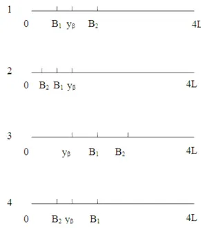
390 Fig. 1: In the subfigure 1(top figure) the bin boundary

B1 is at the left side of the point to be predicted, yp, whereas in the subfigure 2 (bottom figure), the bin boundary, B1 is at the right side of yp

RvC with ERD with three bins: In this case, there are

two bin boundaries; B1 and B2. To calculate the predicted value, we will calculate the mean value of all the predicted values by different models. There are two cases (Fig. 2):

• The bin boundary B1 is left of the given point yp. The two conditions are possible:

• The bin boundary B2 is at the right of the B1. In this case, for different runs B2 is placed at different points between points B1 and 4L. This case is similar to the two bin case with the boundaries; B1 and 4L. Hence, for a given B1, the mean value is yp/2 + (4L + B1)/4 (by using Eq. 2)

• The bin boundary B2 is at the left of the B1. In this case, the predicted values is the center of the rightmost bin, which is (B1 + 4L)/2, this value is independent of B2. Hence, the mean value for a given B1 is (B1 + 4L)/2

The probability of the first condition = (4L-B1)/4L. The probability of the second condition = B1/4L. As B1 can take value from 0 to yp. The mean value of this case (the bin boundary B1 is left of the given point yp) is:

(

)

(

)

(

)

(

)

(

)

(

)

(

)

(

)

p 1

yp

p 1 1

0

1

y / 2 4L B / 4

(1 / y ) 4L B / 4L dB

B1 4L / 2 B / 4L

⎛ ⎛ + + ⎞ ⎞

⎜ ⎜ ⎟ ⎟

⎜ ⎜ ₋ ₊ ⎟ ⎟

⎜ ⎜ ⎟ ⎟

⎜ ⎜ ₊ ⎟ ⎟

⎜ _⎝ _⎠ ⎟

⎝ ⎠

∫

(5)

= -(yp)2/24L + 3yp/4 + L (6)

Fig. 2: (1) The first bin boundary B1 is at the left side of the yp. The second bin boundary B2 is at the right side B1. (2) The first bin boundary B1 is at left side of the yp. The second bin boundary B2 is at the left side B1. (3) The first bin boundary B1 is at the right side of the yp. The second bin boundary B2 is at the right side B1. (4) The first bin boundary B1 is at the right left side of the yp. The second bin boundary B2 is at the left side B1

• The bin boundary B1 is at right of the given point yp. The two conditions are possible:

• The bin boundary B2 is at the right of the B1. In this case, the predicted values is the center of the leftmost bin, which is (B1)/2. Hence, the mean value, for a given B1, is (B1)/2

• The bin boundary B2 is at the left of the B1. In this case, for different runs B2 is placed at different points between points 0 and B1. This case is similar to the two bin case with the range of the target variable between 0 and B1. Hence, the mean value, for a given B1 is, yp/2 + (0 + B1)/4

The probability of the first case = (4L - B1)/4L. The probability of the second case = B1/4L.

As B1 can take value from yp to 4L. The mean value of this case (the bin boundary B1 is at right of the given point yp) is:

(

)

4L

(

₍

)(

₎

₍

)

₎

1 1

p 1

yp p 1 1

B / 2 4L B / 4L 1

/ 4L y dB

y / 2 B / 4 B / 4L

⎛ − + ⎞

⎜ ⎟

−

⎜ + ⎟

⎝ ⎠

(5)

= -(yp)2/24L + 5yp/12 + 3L/4 (8)

The mean value of all the cases: (The mean value of

case 1)(The probability of case 1) + (The mean value of case 2)(The probability of case 2):

( )

(

)

( )

(

)

(

)

2

p p p

2

p p p

y / 24L 3y / 4 L y / 4L

y / 24L 5y / 12 3L / 4 4L y / 4L

= − + + +

− + + − (9)

= yp/2 + ( 2L/3 + (yp)2/8L - (yp)2/48L2 ) (10) For yp = 0 the predicted value is 2L/3.

For yp = 2L the predicted value is 2L. For yp = 4L the predicted value is 14L/3.

The MSE for this case is:

( )

2 2 4L

p

2 ₂

0

p

2L / 3 y 1

/ 4L y – ( y / 2 dy) /8L y / 48L

⎛ ⎛ ₊ ⎞⎞

⎜ ₊ ⎜ ⎟⎟

⎜ ⎜_⎜ ⎟_⎟⎟

⎜ _⎝ − _⎠⎟

⎝ ⎠

∫

(11)

MSE = 0:12L2 (for 4L = 100, the MSE is 75), which is better than RvC with the equal-width method with three bins (MSE = 0:14L2). This proves that the ensembles with the proposed ensemble method performs better than single model with equal-width discretization for RvC, if the number of bins is 3. One may follow the same kind of calculation to extend these results for bins more than 3. It will be cumbersome but straightforward calculation. As 3 bins, improves the performance of ERD ensembles more as compared to single model with equal-width discretization, we may suggest intuitively that the larger number of bins will give more performance advantage to the proposed ensemble method.

RESULTS

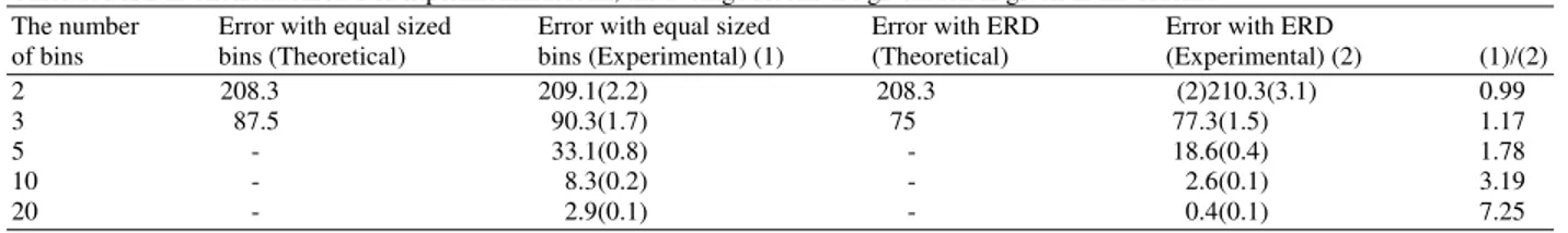
We carried out experiments with y = x function. This is a uniformly distributed function. We generated 10000 points between 0<=x<=100, 5000 points were used for training and 5000 points were used for testing. We used unpruned C4.5 decision tree (J48 decision tree of WEKA software (Witten and Frank, 2005)) as the classifier. The final result from a classifier was the mean value of the target variable (y in this case) of all the points in the predicted bin. In the results, we found that the classification error was almost 0. As in these experiments all the conditions of our theoretical results were fulfilled, we expected that experimental results should follow the theoretical results. We carried out

experiments with two bins and three bins. The size of the ensemble was set to 100. The experiments were conducted following 5×2 cross-validation. The average results are presented in the Table 1. Results suggest that there is an excellent match in experimental results with theoretical results for two bins and three bins cases. We also carried out experiments with 5, 10 and 20 bins. Results suggest that the ratio of the average MSE of RvC with equal-width discretization to the average MSE of RvC with ERD is increasing with the number of bins. This suggests that there is more performance advantage with ERD when we have large number of bins. This verifies our intuition that as we increase the number of bins the performance advantage increases for ERD ensembles. We also carried out experiments with other popular datasets used for regression studies. We also did experiments with REP regression trees (available in WEKA software) with the Bagging procedure. The size of the ensembles was set to 100 for all the experiments. The number of bins was set to 10 for RvC methods.

DISCUSSION

(6)

392

Table 1: MSE in different cases. For experimental results, the average results are given. s.d. is given in the bracket.

The number Error with equal sized Error with equal sized Error with ERD Error with ERD

of bins bins (Theoretical) bins (Experimental) (1) (Theoretical) (Experimental) (2) (1)/(2)

2 208.3 209.1(2.2) 208.3 (2)210.3(3.1) 0.99

3 87.5 90.3(1.7) 75 77.3(1.5) 1.17

5 - 33.1(0.8) - 18.6(0.4) 1.78

10 - 8.3(0.2) - 2.6(0.1) 3.19

20 - 2.9(0.1) - 0.4(0.1) 7.25

Table 2: Experimental results for different methods for different datasets. The average results for RMSE are presented. s.d. is given in the bracket

RvC with Bagging with REP

Name of dataset RvC with ERD equal-width bins Regression trees

Abalone 2.24(.05) 2.89(0.08) 2.17(.05)

Bank8FM 3.61(.11)×10−2_5.31(0.17)_×₁₀−2_3.52(.12)_×₁₀−2

Cart 1.06(.02) 1.46(0.06) 1.05(0.03)

Delta(Ailerons) 1.72(.03)×10−4 2.75(0.05)×10−4 2.03(0.03)×10−4

Delta(Elevator) 1.52(.02)×10−3_1.91(0.03)_×₁₀−3_1.55(0.02)_×₁₀−3

House(8L) 3.12(.05)×104_4.12(.08)_×₁₀4_3.06(.03)_×₁₀4

House(16H) 3.51(.07)×104_4.62(.10)_×₁₀4_3.55(.05)_×₁₀4

Housing(Boston) 3.98(.09) 5.23(0.12) 4.01(0.10)

Kin8nm 0.17(0.01) 0.24(0.02) 0.17(0.01)

Puma8NH 3.28(0.04) 4.50(0.06) 3.25(0.04)

Puma32H 8.21(0.13)×10−3_1.2(.04)_×₁₀−2_7.94(0.17)_×₁₀−3

CONCLUSION

In supervised learning, the target values may be continuous or a discrete set of class. The continuous target values (the regression problem) can be transferred to a discrete set of classes (the classification problem). The discretzation process is a popular method to achieve this task. In this study, we proposed a ensemble method for RvC problems. We showed theoretically that the proposed ensemble method performed better than a single model with equal-width discretization method. This is also verified with experiments. Experiments results also suggest that our method performed similar to the method developed for the regression purpose. This suggests that the proposed ensemble method is useful for regression problems. As the proposed method is independent of the choice of the classifier, various classifiers can be used with the proposed method to solve the regression method. In the study, we carried out experiments with the decision trees, however, in future we will do the experiments with other classifiers like naive Bayes and support vector machines to study its effectiveness with other classifiers.

REFERENCES

Abdulsalam, H., D.B. Skillicorn and P. Martin, 2011. Classification using streaming random forests. IEEE Trans. Know. Data Eng., 23: 22-36. DOI: 10.1109/TKDE.2010.36

Ahmad, A. and L. Dey, 2005. A feature selection technique for classificatory analysis. Patt. Recog.

Lett., 26: 43-56. DOI: 10.1016/j.patrec.2004.08.015

Ahmad, A. and G. Brown, 2009. Random ordinality ensembles: A novel ensemble method for multi-valued categorical data. Multiple Classifier Syst., 5519: 222-231. DOI: 10.1007/978-3-642-02326-2_23 Ahmad, A., 2010. Data transformation for decision tree

ensembles. Ph.D. thesis, School of Computer Science, University of Manchester. http://www.cs.man.ac.uk/~gbrown/publications/ah madPhDthesis.pdf

Alfred, R., 2010. Summarizing relational data using semi-supervised genetic algorithm-based clustering techniques. J. Comput. Sci., 6: 775-784. DOI: 10.3844/jcssp.2010.775.784

Bishop, C.M., 2006. Pattern Recognition and Machine Learning. 1st Edn., Springer-Verlag, New York, ISBN-10: 9780387310732, pp: 738.

Breiman, L., 1996. Bagging predictors. Mach. Learn., 24: 123-140. DOI: 10.1023/A:1018054314350 Breiman, L., 2001. Random forests. Mach. Learn., 45:

5-32. DOI: 10.1023/A:1010933404324

Breiman, L., J. Friedman, R. Olshen and C. Stone, 1984. Classification and Regression Trees. 1st Edn., Chapman and Hall, London, ISBN-10: 0412048418, pp: 358.

Burges, C.J.C., 1998. A tutorial on support vector machines for pattern recognition. Data Min. Knowl. Discovery, 2: 121-167. DOI: 10.1023/A:1009715923555

(7)

Dougherty, J., R. Kahavi and M. Sahami, 1995. Supervised and unsupervised discretization of continuous features. Proceedings of the 12th International Conference on Machine Learning. (ICML’95), Morgan Kaufmann, pp: 194-202. Fan, W., H. Wang, P.S. Yu and S. Ma, 2003. Is

Random model better? On its accuracy and efficiency. Proceedings of 3rd IEEE International Conference on Data Mining, Nov. 19-22, Hawthorne, NY, USA., pp: 51-58. DOI: 10.1109/ICDM.2003.1250902

Fan, W., J. McCloskey and P.S. Yu, 2006. A general framework for accurate and fast regression by data summarization in random decision trees. Proceedings of the 12th ACM SIGKDD International Conference on Knowledge Discovery and Data Mining, (ICKDM’06), ACM New York, NY, USA., pp: 136-146. DOI: 10.1145/1150402.1150421

Freund, Y. and R.E. Schapire, 1997. A decision-theoretic generalization of on-line learning and an application to boosting. J. Comput. Syst. Sci., 55: 119-139. DOI: 10.1006/jcss.1997.1504

Geurts, P., D. Ernst and L. Wehenkel, 2006. Extremely randomized trees. Mach. Learn., 63: 3-42. DOI: 10.1007/s10994-006-6226-1

Halawani, S.M. and I.A. Albidewi, 2010. Recognition of hand printed characters based on simple geometric features. J. Comput. Sci., 6: 1512-1517. DOI: 10.3844/jcssp.2010.1512.1517

Hansen, L.K. and P. Salamon, 1990. Neural network ensembles. IEEE Trans. Patt. Anal. Mach. Intell., 12: 993-1001. DOI: 10.1109/34.58871

Indurkhya, N. and S.M. Weiss, 2001. Solving regression problems with rule-based ensemble classifiers. Proceedings of the 7th ACM International Conference Knowledge Discovery and Data Mining, (KDD’01), ACM New York, NY, USA., pp: 287-292. DOI: 10.1145/502512.502553

Ishrat, R., R. Parveen and S.I. Ahson, 2010. Pattern trees for fault-proneness detection in object-oriented software. J. Comput. Sci., 6: 1078-1082. DOI: 10.3844/jcssp.2010.1078.1082

Kohonen, T., 1989. Self Organization and Associative Memory. 3rd Edn., SpringerVerlag, Berlin, Germany, ISBN-10: 0387513876, pp: 312.

Kuncheva, L.I., 2004. Combining Pattern Classifiers: Methods and Algorithms. 1st Edn., Wiley-Interscience, New York, ISBN-10: 0471210781, pp: 350.

Merckt, T.V.D., 1993. Decision trees in numerical attribute spaces. Proceedings of the 13th International Joint Conference on Artificial Intelligence, pp: 1016-1021.

Minku, L., X. Yao, 2011. DDD: A New Ensemble Approach For Dealing With Concept Drift. IEEE Trans. Know. Data Eng., 99: 1-1. DOI: 10.1109/TKDE.2011.58

Mitchell, T.M., 1997. Machine Learning. 1st Edn., McGraw-Hill, New York, ISBN-10: 0070428077, pp: 414.

Quinlan, J.R., 1993. C4.5: Programs for Machine Learning. 1st Edn., Morgan Kaufmann Publishers Inc., San Francisco, CA, USA., ISBN-10: 1-55860-238-0, pp: 302.

Rodriguez, J.J., L.I. Kuncheva and C.J. Alonso, 2006. Rotation forest: A new classifier ensemble method. IEEE Trans. Patt. Anal. Mach. Intell., 28: 1619-1630. DOI: 10.1109/TPAMI.2006.211

Torgo, L. and J. Gama, 1996. Regression by classification. Advan. Artificial Intell., 1159: 51-60. DOI: 10.1007/3-540-61859-7_6

Torgo, L. and J. Gama, 1997a. Regression using classification algorithms. Intell. Data Anal., 1: 275-292. DOI: 10.1016/S1088-467X(97)00013-9 Torgo, L. and J. Gama, 1997b. Search-based class

discretization. Mach. Learn., 1224: 266-273. DOI: 10.1007/3-540-62858-4_91

Tumer, K. and J. Ghosh, 1996. Error correlation and error reduction in ensemble classifiers. Connect. Sci., 8: 385-404.

Vapnik, V., 1998. Statistical Learning Theory. 1st Edn., Wiley, New York, ISBN-10: 0471030031, pp: 736. Witten, I.H. and E. Frank, 2005. Data Mining: Practical

Machine Learning Tools and Techniques. 3rd Edn., Elsevier Science, New York, ISBN-10: 9780123748560, pp: 650.