Joint retrieval of aerosol and water-leaving radiance from multispectral, multiangular and polarimetric measurements over ocean

(1)

www.atmos-meas-tech.net/9/2877/2016/ doi:10.5194/amt-9-2877-2016

Joint retrieval of aerosol and water-leaving radiance from

multispectral, multiangular and polarimetric

measurements over ocean

Feng Xu1, Oleg Dubovik2, Peng-Wang Zhai3, David J. Diner1, Olga V. Kalashnikova1, Felix C. Seidel1, Pavel Litvinov2, Andrii Bovchaliuk2, Michael J. Garay1, Gerard van Harten1, and Anthony B. Davis1

1_{Jet Propulsion Laboratory, California Institute of Technology, Pasadena, California, USA}

2_{Laboratoire d’Optique Atmosphérique, UMR8518, CNRS/Universite Lille-1, Villeneuve d’Ascq, France} 3_{Department of Physics, University of Maryland, Baltimore County, Baltimore, Maryland, USA}

Correspondence to:Feng Xu (feng.xu@jpl.nasa.gov)

Received: 15 December 2015 – Published in Atmos. Meas. Tech. Discuss.: 18 January 2016 Revised: 27 May 2016 – Accepted: 2 June 2016 – Published: 8 July 2016

Abstract.An optimization approach has been developed for simultaneous retrieval of aerosol properties and normalized water-leaving radiance (nLw) from multispectral, multian-gular, and polarimetric observations over ocean. The main features of the method are (1) use of a simplified bio-optical model to estimate nLw, followed by an empirical refinement within a specified range to improve its accuracy; (2) im-proved algorithm convergence and stability by applying con-straints on the spatial smoothness of aerosol loading and Chlorophylla(Chla) concentration across neighboring im-age patches and spectral constraints on aerosol optical prop-erties and nLw across relevant bands; and (3) enhanced Jaco-bian calculation by modeling and storing the radiative trans-fer (RT) in aerosol/Rayleigh mixed layer, pure Rayleigh-scattering layers, and ocean medium separately, then cou-pling them to calculate the field at the sensor. This approach avoids unnecessary and time-consuming recalculations of RT in unperturbed layers in Jacobian evaluations. The Markov chain method is used to model RT in the aerosol/Rayleigh mixed layer and the doubling method is used for the uni-form layers of the atmosphere–ocean system. Our optimiza-tion approach has been tested using radiance and polar-ization measurements acquired by the Airborne Multiangle SpectroPolarimetric Imager (AirMSPI) over the AERONET USC_SeaPRISM ocean site (6 February 2013) and near the AERONET La Jolla site (14 January 2013), which, respec-tively, reported relatively high and low aerosol loadings. Validation of the results is achieved through comparisons to AERONET aerosol and ocean color products. For

com-parison, the USC_SeaPRISM retrieval is also performed by use of the Generalized Retrieval of Aerosol and Surface Properties algorithm (Dubovik et al., 2011). Uncertainties of aerosol and nLw retrievals due to random and systematic in-strument errors are analyzed by truth-in/truth-out tests with three Chla concentrations, five aerosol loadings, three dif-ferent types of aerosols, and nine combinations of solar inci-dence and viewing geometries.

1 Introduction

(2)

When aerosol is a major target of retrieval, water-leaving radiance is often empirically estimated or even neglected in operational algorithms employed by current-generation satellite imagers due to their small contribution to TOA signals. For examples, the MODIS Collection 5 algorithm uses zero water-leaving radiance for all but the 550 nm band, where a value of reflectance 0.005 is assumed (ρ550 nm=0.005, cf. Remer et al., 2005, 2006). MISR and

POLDER assume zero water-leaving radiance in the red and NIR bands for aerosol retrieval (Kahn et al., 2010; Deuzé et al., 2000). Then observations are searched within a lookup ta-ble (LUT), which contains precalculated radiation fields for a limited number of aerosol models. The aerosol model with lowest fitting residue is selected as the solution. Depending on the sensitivity of measurements, different types and com-binations of aerosol models have been designed. For exam-ple, MODIS LUT has 20 combinations of fine and coarse aerosol models for retrieving aerosol information from mul-tispectral radiance-only observations (Remer et al., 2005, 2006); MISR LUT has 74 aerosol mixtures for retrieving multiangle multispectral radiance-only observations (Kahn et al., 2010); POLDER LUT consists of 12 aerosol models for retrieving multiangle, multispectral, and polarimetric ob-servations (Deuzé et al., 2000).

As the main disadvantage of LUT approach, the solu-tions have to be selected from a finite number of aerosol models which might not be sufficiently representative in the relevant parameter space. New research efforts have been proposed to expand the LUT to cover more aerosol mod-els (e.g., Limbacher and Kahn, 2014). An alternative to the LUT approach is optimization-based retrieval. It involves a direct inversion of the measurements within the context of a parametric description of the aerosol and surface charac-teristics that govern the radiation field observed at the TOA. The optimization-based retrieval is featured by a more com-pact and continuous representation of the relevant parameter space. A review of modern aerosol retrieval algorithms used by airborne and satellite-borne passive remote sensing instru-ments has been recently given by Kokhanovsky (2015).

When water-leaving radiance becomes the major target of retrieval, traditional retrievals decouple the atmosphere and surface using “atmospheric correction” procedures. The Ocean Biology Processing Group (OBPG) uses the atmo-spheric correction developed by Gordon and Wang (1994) and Gordon (1997) and refined by Ahmad et al. (2010). In this algorithm an aerosol optical property lookup table is built for ten aerosol models and eight relative humidity (RH) values based on the aerosol property statistics from Aerosol Robotic Network (AERONET) observations (Ahmad et al., 2010). Aerosol optical depth (AOD) and type are determined by fitting the observations in two near-infrared bands (e.g., 748 and 869 nm for MODIS), where water-leaving radiance is assumed negligible. The selected aerosol model is then ex-trapolated to shorter-wavelength visible bands and applied to the measured TOA radiances to retrieve normalized

water-leaving radiance (nLw) (Gordon and Wang, 1994; Gordon, 1997). To reduce errors caused by this atmospheric correc-tion procedure and instrumental radiometric uncertainties, empirical gain factors are derived by forcing agreement be-tween retrieved nLw values and in situ measurements ob-tained at the Marine Optical Buoy (MOBY) site in Lanai, Hawaii (Franz et al., 2007).

For single-angle, nonpolarimetric instruments such as MODIS and the Sea-Viewing Wide Field-of-View Sensor (SeaWiFS), Franz et al. (2007) pointed out that, “the perfor-mance of satellite-based ocean color retrieval process is rela-tively insensitive to the aerosol model assumption . . . at least for open-ocean conditions where maritime aerosols dominate and aerosol concentrations are relatively low (i.e., aerosol optical thickness generally less than 0.3 at 500 nm)”. There-fore, the gain factors derived from conditions at the MOBY site can be applied globally to improve the agreement be-tween satellite and in situ nLw over deep (Case 1) waters. In more challenging observing conditions, e.g., in the presence of absorbing aerosols or complex, spatially diverse (Case 2) waters, inaccurate knowledge of the absorbing aerosol op-tical properties or height distribution can lead to incorrect assumptions regarding CDOM and phytoplankton absorp-tion coefficients (Moulin et al., 2001; Schollaert et al., 2003; Banzon et al., 2009). In addition, the vertical distribution of absorbing aerosols can affect the reflectance of the ocean– atmosphere system, resulting in errors in nLw (Duforêt et al., 2007). In coastal regions, where the traditional assumption of zero water-leaving radiance in the near-infrared (NIR) (Gor-don, 1997; Siegel et al., 2000) breaks down, backscattering from suspended hydrosol particles (e.g., algae or sediment) can be misinterpreted as aerosols, leading to overestimation of AOD. The resulting overcorrection can lead to underesti-mated or even negative water-leaving radiances in the blue and green (e.g., Hu et al., 2000; Bailey et al., 2010; He et al., 2012).

(3)

polarimetry in the retrieval enables retrieval of aerosol types that may be beyond the capabilities of the LUT and poten-tially improves accuracy of both the aerosol and ocean wa-ter properties. Given that measurements of atmospheric min-eral dust and carbonaceous aerosols show a strong spectral dependence of absorption coefficient in the near-UV (e.g., Koven and Fung, 2006; Bergstrom et al., 2007; Russell et al., 2010) and have a spectral signature similar to those of CDOM, accurate modeling of radiative transfer (RT) in the coupled atmosphere–ocean system (CAOS) becomes neces-sary.

Without using bio-optical models, some RT models for CAOS consider specular reflection by assuming a flat ocean surface (Jin and Stamnes, 1994; Bulgarelli et al., 1999; Chami et al., 2001; Sommersten et al., 2009; Zhai et al., 2009) for simplicity. Better modeling fidelity and accuracy is then achieved by including sea surface roughness into the RT models (Nakajima and Tanaka, 1983; Fischer and Grassl, 1984; Masuda and Takashima, 1986; Kattawar and Adams, 1989; Mobley, 1994; Deuzé, 1989; Jin et al., 2006; Spurr, 2006) and including the water-leaving radiance and/or ocean foam reflection based on a Lambertian or a more general bidirectional reflectance distribution model (Koepke, 1984; Lyapustin and Muldashev, 2001; Mobley et al., 2003; Sayer et al., 2010; Sun and Lukashin, 2013; Gatebe et al., 2005). Though empirical parameterization of water-leaving radiance simplifies the radiative transfer, the relationship be-tween water-leaving radiance and inherent optical properties (IOP) of dissolved or suspended ocean constituents is indi-rect. Such a weakness can be overcome by using bio-optical models to relate IOP directly to water-leaving radiance. The bio-optical model-based RT methods make it feasible to per-form a one-step retrieval of IOP and aerosol optical proper-ties from TOA measurements of radiance and polarization (e.g., Hasekamp et al., 2011), which is a complementary re-trieval strategy to the prevailing two-step rere-trieval that ob-tains nLw from TOA via atmospheric correction and then determines IOP from nLw (IOCCG, 2006). Various RT solu-tions involving the use of bio-optical models have been de-veloped and can be used for this purpose. These include the invariant imbedding method adopted by HydroLight (Mob-ley, 2008) and its faster version EcoLight (Mob(Mob-ley, 2011a) for scalar (intensity only) RT, in addition to the adding– doubling method (Chowdhary et al., 2006) and successive-order-of-scattering method (Zhai et al., 2010) for polarized RT in the CAOS.

Joint retrieval of aerosol and nLw properties requires sup-plementing the forward RT calculations with a sophisticated and computationally efficient inverse model to disentangle their contributions to TOA radiometry and polarimetry. Moti-vated by the development of a multiangle imaging polarime-ter at JPL – the Airborne Multiangle SpectroPolarimetric Im-ager (AirMSPI) (Diner et al., 2013) – this paper describes the development of a coupled aerosol-ocean retrieval methodol-ogy. Our method (1) employs a simplified bio-optical model

to obtain a reasonable estimate of nLw in the first retrieval step, followed by an empirical refinement in the subsequent step; (2) applies constraints on the spatial smoothness of aerosol and Chl loadings across neighboring image patches and spectral constraints on aerosol optical properties and on nLw across relevant bands to improve the convergence and stability of the algorithm; and (3) models and stores the RT fields in the aerosol/Rayleigh mixed layer, the pure Rayleigh-scattering layers, and the ocean medium separately, then couples them to obtain the radiative field at the sensor – thereby enhancing the Jacobian evaluations by reusing RT fields in the unperturbed layers. The Markov chain and dou-bling methods are applied to the mixed and uniform layers, respectively, to gain computational efficiency.

The parameters of our retrieval include spectrally depen-dent real and imaginary parts of aerosol refractive index, aerosol concentrations of different size components, mean height and width of aerosol distribution, nonspherical par-ticle fraction, wind speed over ocean surface, and normal-ized water-leaving radiance. As auxiliary product, aerosol phase matrix is obtained from the retrieved refractive index and normalized size distribution. Throughout the paper, we use the definition of “exact” normalized water-leaving radi-ance (nLw) given by Morel et al. (2002). It is consistent with the definition adopted by Franz et al. (2007) and Zibordi et al. (2009) and is related to the remote sensing reflectance (Rrs)byRrs=nLw/F0, whereF0is the extraterrestrial

so-lar irradiance.

The paper is organized as follows. In Sect. 2, we introduce our development of the RT model that integrates the Markov chain, doubling and adding methods for CAOS. The multi-patch retrieval algorithm is described in Sect. 3. In Sect. 4, a truth-in/truth-out test is performed to assess the retrieval un-certainties for a variety of synthetic scenarios combined from three types of aerosols, five aerosol loadings, three Chl a concentrations, three solar incidence angles, four viewing ge-ometries, and two types of measurement noise. To test the al-gorithm with real data, retrievals applied to AirMSPI obser-vations over the USC_SeaPRISM AERONET site and near the La Jolla AERONET site are compared to the independent AERONET results. A summary is presented in Sect. 5.

2 A integrated radiative transfer model for a coupled atmosphere–ocean system

(4)

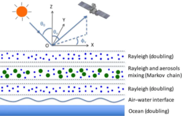
Figure 1.Depiction of the 5-layer CAOS model. A Gaussian ver-tical distribution profile for aerosols in the mixed layer is assumed and the Markov chain model is used for RT in this optically inho-mogeneous layer. The ocean medium and the two Rayleigh layers (below and above the mixed layer, respectively) are treated as op-tically homogeneous and the doubling method is used for the RT computations. Coupling of these layers and inclusion of the air– water interface are completed by use of the adding strategy. The Sun illuminates the top-of-atmosphere with solar zenith angle θ0

and azimuthal planeφ0. We defineφ=φv−φ0, where the sensor

views the atmosphere at viewing angleθvand azimuthal angleφv.

and single scattering properties of aerosols in the mixed layer are demonstrated in Appendix A.

2.1 Radiative transfer modeling and Jacobian evaluation strategy

The five-layer CAOS model allows the use of different RT methods to model radiative transfer in different layers based on their computational strength. As an example, the Markov chain method (Esposito and House, 1978; Xu et al., 2010, 2011, 2012), which exhibits high computational efficiency for modeling RT in vertically inhomogeneous media (Espos-ito, 1979), is adopted in this work for the aerosol/Rayleigh mixed layer (see Appendix B for details). The doubling method (Stokes, 1862; van de Hulst, 1963; Hansen, 1971; de Haan et al., 1987; Evans and Stephens, 1991; among oth-ers), which exhibits high efficiency for modeling RT in op-tically homogeneous media (Esposito, 1979) is used for the two pure Rayleigh layers and the ocean medium (assumed to be homogeneous throughout the paper). Appendix C gives an example of using the doubling method for modeling RT in the ocean medium. The radiative fields from all layers are then coupled using an adding strategy to obtain the TOA fields.

In addition to the benefit of enabling a combination of the strengths of different RT methods, the strategy of sepa-rate RT modeling in five layers also makes for an efficient optimization-based retrieval. During the iterative optimiza-tion process, Jacobians are calculated to represent how the

radiation fields vary as a function of the model parameters. When they are evaluated by perturbing a model parameter within one of the layers, the diffuse RT fields for all other layers are unchanged from the values obtained from the for-ward RT simulation and thus can be reused. For example, calculation of the Jacobians with respect to surface or ocean bio-optical parameters does not require recomputation of RT in the atmospheric layer because it has already been de-rived from the previous forward model calculation. Similarly, when evaluating Jacobians with respect to the aerosol param-eters, it is unnecessary to repeat the RT computation of the Rayleigh layers and in the ocean or at the air–water interface. Because optimization-based retrievals involve Jacobian eval-uations for a large number of parameters at all iterative steps, this strategy significantly improves the retrieval efficiency. 2.2 Atmosphere–ocean coupling

For the atmosphere, the diffuse radiative fields for the aerosol/Rayleigh mixed layer and the pure Rayleigh lay-ers are computed by Markov chain and doubling methods, respectively, then coupled to get the diffuse reflection and transmission matrices for the whole atmosphere (see Ap-pendix B).

For the ocean, the radiative field in the bulk medium is computed by the doubling method with the optics of ocean constituents evaluated by use of a simplified bio-optical model (see Appendix D), then coupled with the re-flection and transmission across the air–water interface, and finally corrected to account for Raman scattering (see Ap-pendix C). In addition to the contribution by water-leaving radiance from the simplified bio-optical model, total light leaving ocean surface also includes polarized specular re-flection (RW, see Appendix E), a Lambertian term for

de-polarizing ocean foam reflection and an empirical Lamber-tian correction term,1aWL, to account for the errors of the

single-parameter-based bio-optical model for water-leaving radiance (i.e., departures from the predetermined functional relationships to Chla concentration). Thus, the overall bidi-rectional ocean surface reflection matrixRsurf is described

as

πRsurf=ffoamafoamD0+(1−ffoam)RW (1) +(1−ffoam)RBioWL+(1−ffoam)1aWLD0,

whereD0 is a zero matrix exceptD0,11=1,afoam is foam

albedo,ffoamis foam coverage fraction related to wind speed Wbyffoam=2.95×10−6×W3.52(Koepke, 1984), andRBioWL

is the reflection matrix of the ocean-interface system with Raman-scattering correction (see Appendix C). Note that RBio_WL is a physically based term in which Chl a concentra-tion ([Chl_a]) is an adjustable free parameter. The last two terms of Eq. (1) constitute our water-leaving radiance model. With and without assuming 1aWL to be 0 the simplified

(5)

in Eq. (1) has angular dependence, to be consistent with the conventional ocean color products we derive fromRBio_WLand 1aWL in Eq. (1) the normalized water-leaving radiance by

setting the Sun at zenith (θ0=0◦) and viewing angle to be

nadir (θv=0◦):

nLw₌ (2)

F0 π

_d

0 d

2h

R_WL,11Bio (θv=0◦;θ0=0◦; [Chl_a])+1aWL

i

,

whered0is the Earth–Sun distance at which the solar

irradi-ance F0 is reported, andd is the Earth–Sun distance at the

time of measurement. Note that nLw,RW,Rsurf,RBioWL,afoam, 1aWL, andF0in Eqs. (1)–(2) are all spectrally dependent.

Once the diffuse reflection and transmission matrices of the atmosphere and reflection from ocean system are individ-ually known, their coupling to get RT field for the full CAOS is implemented by using the adding method. Two operators QandSare defined to account for the interaction between the ocean and atmosphere via single and higher orders of re-flection, respectively:

Q1=R∗atmosRsurf (3a)

Qn=Q1Qn−1 (3b)

S₌

∞

X

n=1

Qn, (3c)

whereRsurfis the diffuse reflection matrix from ocean

sur-face andR∗_atmos is the diffuse reflection matrix from sphere with light illumination from the bottom of the atmo-sphere. The matrices for downwelling and upwelling diffuse light at the atmosphere–ocean interface are given by

D₌Tatmos+Sexp

−τatmos µ0

+STatmos (3d)

U₌Rsurfexp

−τatmos µ0

+RsurfD, (3e)

whereµ0=cosθ0. The reflection matrix of the full CAOS is

RCAOS=Ratmosexp

−τatmos_µ

U₊T∗_atmosU, (3f)

whereµ_{= |}cosθ_|. For simplicity in describing the concep-tual scheme, the superscript “m” that denotes Fourier series order was not shown in the above expression. In actuality, the TOA radiation fields are reconstructed from all orders of

Fourier terms: BRFtot=π

∞

X

m=0

(2−δ0m)R(m)_CAOS_,₁₁cosmφ (4a)

qBRF_tot=π ∞

X

m=0

(2−δ0m)R(m)_CAOS_,₂₁cosmφ (4b)

uBRFtot=π ∞

X

m=0

(2−δ0m)R(m)_CAOS_,₃₁cosmφ (4c)

vBRFtot=π ∞

X

m=0

(2−δ0m)R(m)CAOS,41cosmφ, (4d)

where the bidirectional reflectance factor BRFtot and

DoLP= √

qBRF2tot+uBRF2tot+vBRF2tot

BRF2 tot

are used to fit the observa-tion. Since the sunlight is unpolarized, other matrix entries (namely RCAOS,ij, with j≥2) are not involved in Stokes

vector calculation for the diffuse light from the reflection ma-trix.

Note that the above formalism for modeling RT in a CAOS assumes a horizontally homogeneous atmosphere above a uniform surface, which is known as the independent pixel/patch approximation (IPA) in RT theory (Cahalan et al., 1994). In reality, however, aerosol properties and surface reflection vary across the pixels/patches. To reduce the IPA errors, the single-scattering contribution to the total field evaluated by Eq. (4) is replaced by an exact evaluation of radiance along the line of sight. Moreover, for simplicity of model demonstration, our five-layer model assumes the sensor to be located at the TOA. For real airborne measurements, however, the sensor is located inside the atmosphere. Therefore to improve the modeling accuracy, the radiative field is actually com-puted at the sensor location. This is realized by adding an extra Rayleigh layer above the sensor altitude (e.g., h > hAirMSPI=20 km in our case), then using theUterm in

the adding method to compute the diffuse upwelling light reaching the sensor. Moreover, ozone correction is made by BRFtot, corr(λ)=BRFtot(λ)exp[−τozone(λ)(1/cosθ0+ fozone/cosθv)], where τozone is the total ozone optical

depth and fozone is the fraction of ozone above the sensor

(in our current study fozone is assumed to be 20 % for hAirMSPI=20 km).

The integrated RT model established in the current section will be used as the forward model in retrieval, which is to be introduced in the next section.

3 Optimization approach for joint aerosol and water-leaving radiance retrieval

(6)

con-tains all relevant parameters characterizing aerosol proper-ties, water-leaving radiance, and surface reflection is ap-proached in an iterative way by xk+1=xk−1xk with xk being the solution after k iterations and 1xk being

the increment being obtained by1xk=(JT_k)−11yk, where

Jk is the Jacobian matrix evaluated with xk, and 1yk is

the difference between model and measurement (1y_k₌ y(xk)−ymeas). Unfortunately, the determinant ofJk is

of-ten close to 0 and as a result Jk is ill conditioned.

There-fore, a stable retrieval that ensures convergence to a phys-ically sensible solution must impose constraints such that det[JT_k(Cf)−1Jk+γk,1Wk,1+γk,2Wk,2+. . .]>0 and1xk=

[JT_k(Cf)−1Jk+γk,1Wk,1+γk,2Wk,2+. . .]−11y′_k, whereCf

is the covariance matrix of the measured signals, Wk,i

de-notes the imposed various constraints,γkis a Lagrange

mul-tiplier that assigns a weight to the constraint, and 1y′_k in-corporates 1y_k and the relevant a priori constraints and Lagrange multipliers. Introduction of various types of con-straints and/or an a priori estimate of W, and establish-ment of a means for determinant γk are key elements of

optimization-based algorithms. Different approaches include the Levenberg–Marquardt algorithm (Levenberg, 1944; Mar-quardt, 1963), the Phillips–Tikhonov–Twomey algorithm (Phillips, 1962; Tikhonov, 1963; Twomey, 1963, 1975), and the Twomey–Chahine algorithm (Chahine, 1968), as dis-cussed by Dubovik et al. (2004).

To maximize the use of information provided by different remote sensing instruments on aerosol and surface proper-ties, various algorithms have been applied to inverse radiance and polarimetric signals (Kokhanovsky, 2015; Kokhanovsky et al., 2015). For the particular application of AirMSPI aerosol and water-leaving radiance retrievals, an adaptation of the inversion approach of Dubovik (2004) and Dubovik et al. (2008, 2011) is used. This approach considers inversion as a multiterm least square fitting with multiple a priori con-straints. Particularly, as suggested by Dubovik et al. (2008, 2011), additional constraints on temporal or spatial variabil-ity of the retrieved characteristics can be used if the re-trieval is performed for a group of observed pixels/patches. In the present application, a smoothness constraint is im-posed to constrain spatial variation of aerosol properties and Chla concentration over a target area of finite size. While the term “multipixel algorithm” is introduced by Dubovik et al. (2011) for POLDER/PARASOL retrievals with pixel data of∼6 km×7 km resolution at nadir, the term “multi-patch algorithm” is used here since the AirMSPI pixel res-olution is much finer (10 m×10 m) and 50×50 pixels are merged into a “patch” to reduce IPA errors. Moreover, as an extension of what is meant by multispectral and multiangle, even polarimetric, a multipixel algorithm can be understood as one based on a forward signal model that can predict how radiances escaping from different pixels are physically cou-pled, which is tantamount to using 3-D RT (cf. Langmore et al., 2013, for a background-aerosol and gas-plume retrieval

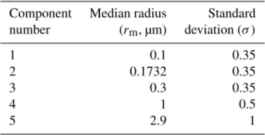
Table 1.Median radius (rm)and standard deviation (σ )ofNsc=5

volume weighted log-normal size components, namely dvi(r)/d lnr

in Eqs. (A4)–(A5).

Component Median radius Standard number (rm, µm) deviation (σ )

1 0.1 0.35

2 0.1732 0.35

3 0.3 0.35

4 1 0.5

5 2.9 1

demonstration). To avoid confusion, we use the terminology “multipatch” here.

Note that though accurate forwarding RT modeling with multiple aerosol species is possible, the increased number of free parameters challenges the ability to retrieve a glob-ally optimized solution in an efficient way. Therefore, as de-scribed in Appendix A, a single aerosol species is assumed to represent an effective set of aerosol optical properties, size distribution (which may be multimodal), and vertical profile. Five log-normal size distribution components (Nsc=5) are

used to represent the aerosol size distribution, with median radii and standard deviations optimally chosen and given in Table 1, and size-independent refractive index are as-sumed. Retrieval with more than five size components has also been performed and comparison shows that they both retrieve well aerosol optical properties after being optimally set as log-normally shaped (Dubovik et al., 2006). Since five-component-based retrieval is faster, it is adopted in the cur-rent study. Nevertheless, our retrieval leaves the option open for adopting more than five components as well as for retriev-ing size-dependent refractive index when extra constraints or sensitivity from observation in some observation cases are available.

In the next three subsections, we will give some details on the design of a multipatch retrieval algorithm for joint aerosol and water-leaving radiance retrieval. Readers not interested in it could skip over them.

3.1 Multipatch retrieval algorithm with smoothness constraints

(7)

N-patch image (Dubovik et al., 2011).

C(x)₌

N X

i=1

9(xi)+

1 2x

T

interpatchx (5)

=

N X

i=1

[9f(xi)+9s(xi)+9a(xi)]+

1 2x T interpatchx =1 2 N X

i=1

h

1yT_iW−_f_,i11y_i₊γsxTis,ixi

+γa(xi−x∗i)TW−

1

a,i(xi−x∗i) i

+1

2x

T

interpatchx,

where xi is an iterative solution for the set of parameters

being retrieved and x∗_i is an a priori estimate of the solu-tion corresponding to theith patch,x_{= [}x1,x2,x3, . . .xN]; 9f(xi),9s(xi)and9a(xi)correspond to the residues of

fit-ting observations, the spectral smoothness constraints, and the a priori estimate, respectively;s,i is a smoothness

ma-trix for constraining the spectral variation of aerosol opti-cal properties and water-leaving radiances across the rele-vant bands;WfandWaare the weighting matrices for

mea-surements and the a priori estimate, respectively;γ denotes the relevant Lagrange multipliers;1y_i is the difference be-tween the model and measurements for theith patch [1y_i₌ y(xi)−ymeas]; andinterpatch is the interpatch smoothness

matrix constructed for the patches along two orthogonal di-rections (uandv) of the image, namely

interpatch=γuS(mu),TS(mu)+γvS(mv),TS(mv), (6)

where the derivative matrixS(m)_{is constructed from the}_m_th

order difference, andγuandγvare the Lagrange multipliers

and their values are shown in Table 2 for all retrieval param-eters.

The optimal solution is approached in an iterative way so that afterk iterations, the solution vectorxi,k+1 containing

parameters of aerosol and surface properties for theith patch is updated as

xi,k+1=xi,k−tp1xi,k, (7)

where the multipliertp(0≤tp≤1) is introduced to improve

the convergence of the nonlinear numerical algorithm (Orega and Reinboldt, 1970). Solving the following normal system constructed for theN-patches image at thekth iteration gives

the increment of solution for each patch (1xi,k),        

A1,k 0 . . . 0

0 A2,k . . . 0

. . . .

0 0 . . . AN,k

  

+interpatch,k        

1x1,k

1x2,k

. . . 1xN,k

    =        

∇9(x1,k)

∇9(x2,k)

. . . ∇9(xN,k)

  

+interpatch,k    

x1,k x2,k

. . . xN,k       

, (8)

where the Fisher matrix for theith patch is a function of Ja-cobian matrixJi,kand weighting matrixWf,i,

Ai,k=JTi,kW−f,i1Ji,k+γs,i,k1,i+γa,i,kW−

1

a,i, (9)

and ∇9(xi,k) is the gradient of the minimized quadratic

form:

∇9(xi,k) =JTi,kW−

1

f,i(yi,k−yi,meas)+γs,i,ks,ixi,k (10)

+γa,i,kW_a−_,i1(xi,k−x∗i),

wherey_meascontains the measurement data,y_kcontains the modeled radiance and polarization withxk,Wfis the

weight-ing matrix defined as the covariance matrixCf normalized

by its first diagonal element namelyWf=(1/σSD2 ,1)C(with σSDbeing the standard deviation),Wais the weighting

ma-trix of the a priori estimatex∗, and s is the

single-patch-based smoothness matrix containing sub-smoothness matri-ces for all parameters. The Lagrange multipliersγs reflects

the strength of the smoothness constraints.

As listed in Table 2, the parameters of the retrieval in-clude spectrally dependent real (mr) and imaginary (mi)

parts of aerosol refractive index, aerosol concentrations of all size components (Cv(rm)), mean height (ha)and half width

(σa) of aerosol layer, nonspherical particle fraction (fns),

wind speed over ocean (W), Chlaconcentration ([Chl_a]), and1aWL, which adjust the nLw values in the second step

of the retrieval. These parameters form the solution vec-tor x₌log[mr(λ), mi(λ), Cv(rm), ha, σa, fns, W, Chl_a, aWL, Const(λ)+1aWL(λ)]T, where the natural logarithm is

used to ensure nonnegativity of the real solution after dy-namic positive or negative changes during the iterative opti-mization process. The termaWL, Constis an offset determined

from nLw using [Chl_a] from the first retrieval step to en-sure that the adjustment of nLw in logarithmic space is real. Thenγss is constructed as a block matrix from diagonal

concatenation of the spectral smoothness matrices for real and imaginary parts of the refractive index and1aλ, namely

for all patches: γss=diag

0,0,0,0,0, γs,mrs,mr, γs,mis,mi,0,0, (11)

0,0,0,0, γs,(aWL,Const+1aWL)s,(aWL,Const+1aWL) ,

(8)

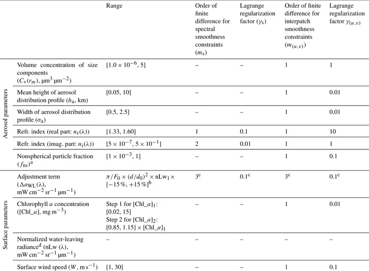
Table 2.Parameters in ocean retrieval and Lagrange multipliers for smoothness constraints.

Range Order of

finite difference for spectral smoothness constraints (ms)

Lagrange regularization factor (γs)

Order of finite difference for interpatch smoothness constraints (m(u,v))

Lagrange regularization factorγ_(u,v)

Volume concentration of size components

(Cv(rm), µm3µm−2)

[1.0×10−6, 5] – – 1 1

Aerosol

parameters

Mean height of aerosol distribution profile (ha, km)

[0.05, 10] – – 1 0.01

Width of aerosol distribution profile (σa)

[0.5, 2.5] – – 1 0.01

Refr. index (real part:nr(λ)) [1.33, 1.60] 1 0.1 1 10

Refr. index (imag. part:n_i(λ)) [5×10−7, 5×10−1] 2 0.01 1 1 Nonspherical particle fraction

(fns)a

[1×10−3, 1] – – 1 0.1

Adjustment term (1aWL(λ),

mW cm−2sr−1µm−1)

π/F0×(d/d0)2×nLw1× [−15 %,+15 %]b

3c 0.1c 3c 0.1c

Surf

ace

parameters

Chlorophyllaconcentration ([Chl_a], mg m−3)

Step 1 for [Chl_a]1:

[0.02, 15]

Step 2 for [Chl_a]2:

[0.85, 1.15]×[Chl_a]1

– – 1 0.01

Normalized water-leaving radianced(nLw (λ), mW cm−2sr−1µm−1)

– – – – –

Surface wind speed (W, m s−1) [1, 30] – – 1 0.1

a_{Nonspherical (spheroidal) particle fraction is excluded in truth-in/truth-out test but included in real data retrieval;}b_{The subscript “1” of nLw means the normalized water-leaving}

radiance determined from Chlaconcentration ([Chl_a]1)retrieved at step 1;cDetermined with the consideration of constant offsetπ/F0×(d/d0)2×nLw1(λ);dThe normalized water-leaving radiance is not directly retrieved. After the second step retrieval, the updated Chlaconcentration [Chl_a]2and the adjustment term1aWLare used to derive it via Eq. (2).

In our retrieval test, an a priori estimate is assumed un-available so we setai,k=a_i,a∗ . Therefore Eq. (10) simplifies

to

∇9(xi,k)=JTi,kW−f,i1(yi,k−yi,meas)+γs,i,ks,ixi,k. (12)

When the spectral and spatial smoothness constraints are turned off (namely settingγs=γu=γv=0), the multipatch

algorithm reduces to the traditional Levenberg–Marquardt algorithm (Levenberg, 1944; Marquardt, 1963), which has been used for retrieval tests with MISR synthetic radiances (Diner et al., 2011; Xu et al., 2012).

Ideally, the retrieval is deemed successful when the mini-mization of the cost function is achieved, such that

2

N_Xpatch

i=1

9(xk,i)+xkinterpatch,kxTk ≤Ninterpatchεf2 (13)

+

N_Xpatch

i=1

(Nf,i+Ns,i+Na*,i−Na,i)εf2,

whereNf,i,Ns,i,Na,i andNa∗,i are the number of

observa-tions, spectral smoothness, number of unknowns, and a pri-ori estimates of parameters corresponding toith patch, re-spectively; Ninterpatch is the number of spatial smoothness

(9)

threshold value,ε_c2. Namely,

ε_c2_≥ (14)

" 2

Npatch_P

i=1

9(xk+1,i)+xk+1interpatch,k+1xTk+1 #

− "

2 Npatch_P

i=1

9(xk,i)+xkinterpatch,kxTk #

2 Npixel_P

i=1

9(xk,i)+xkinterpatch,kxT k

,

is the second criterion to terminate the optimization. 3.2 Determination of Lagrange multipliers

Following Dubovik and King (2000), the Lagrange multipli-ers reflecting the strength of smoothness constraints are de-fined as

γg=εf2/ε 2

gandγa=εf2/ε 2

a, (15)

whereε_f2,ε2_aandε_g2are the first diagonal elements of the co-variance matrices corresponding to the measurements (Cf),

to the a priori estimates (Ca) and to the smoothness

con-straints (Cg, with the subscript “g” indicating the spectral

smoothness constraint “s” or spatial smoothness constraint “u” or “v”), respectively. To estimateε2_gfor a given param-eter to be retrieved (xj), which is a function oft, the most

unsmooth-known solutionx_jns(t )over the target area is used, namely,

ε_g2₌

tZmax

tmin

dm_[x_jus(t )_] dmt

!2

dt, (16)

wheretminandtmaxspecify the lower and upper bound oft.

In practical implementation of our algorithm, however, the Lagrange multipliers are modified in the following way:

γ_gFinal₌ Nf Ng

eε2_f

ε2_fγgandγ Final

a =

Nf Na

eε2_f

ε2_fγa. (17)

There are two differences betweenγ_...Finalandγ...:

1. The multipliersNf/NgandNf/Naare introduced to

ac-count for possible redundancy of the measured and a priori data. Considering thatε2_...is a variance of the er-ror in a single measured or estimated a priori value, if we have N values of similar kind the total variance increases proportionally to N. Introducing this coeffi-cient ensures that when there are several kinds of data, the data with fewer values are given comparable weight as the data type for which there is a greater number of available values.

2. The multiplier_eε_f2/ε2_f is introduced with_eε2_f estimated as the dynamic fitting residual during iterations:

eε_f2(xk)≈ (18)

2

Npatch_P

i=1

9(xk,i)+xkinterpatch,kxT_k

Ninterpatch+

Npatch_P

i=1

(Nf,i+Ns,i+Na*,i−Na,i)

.

With the multipliereε2_f/ε2_f, the fitting residual is used as an estimate of measurement error variance. As a result, during the first few iterations the contribution of the a priori term is strongest, and its influence de-creases as the retrieval progresses. This is done to ensure mostly monotonic convergence, as in the Levenberg– Marquardt procedure (Levenberg, 1944; Marquardt, 1963). However, the Levenberg–Marquardt approach does not specify a particular scheme for introducing these terms, rather it relies on the implementer’s intu-ition. Our algorithm requires the fitting errors in the ini-tial iterations to be dominated by model linearization errors as opposed to random measurement errors. Be-cause at each iterative step the full forward model is replaced by its linear approximation, the errors of lin-earization decrease as convergence toward the final so-lution progresses, and they practically disappear so that

eε_f2becomes equal toε_f2. As a result of this adjustment of the Lagrange multiplier, the nonlinear iteration becomes significantly more monotonic.

3.3 Implementation of two-step retrieval

As water-leaving radiance is a small contribution to TOA signals, opening a large number of parameters for its re-trieval increases the risk of obtaining solutions at local min-ima of the fitting metric and a significant slowdown of the retrieval. To improve retrieval efficiency and reliability, we use a two-step retrieval strategy: obtaining a reasonable es-timate of water-leaving radiance (i.e., close to the truth) by using a bio-optical model constrained by a single parameter (namely Chlorophyll a concentration, [Chl_a] which gov-erns the abundance of CDOM and phytoplankton in a pre-scribed way) during the first step of the retrieval. This is ac-complished by setting1aWLto zero so that only Chla

con-centration (the ocean parameter to which the measurements have the largest information content) is retrieved. Other ocean parameters (e.g., CDOM concentration) are models as dependent on [Chl_a]. In light of the possibility that the bio-optical model parameterized by Chlaconcentration only can have inaccuracies (particularly in Case 2 waters), this con-straint is relaxed in a subsequent step so that the nLw re-trieval is improved by letting the Chlaconcentration and the 1aWLterm be optimized simultaneously (1aλ,WLis allowed

(10)

and atmospheric modeling errors to the water-leaving radi-ance, the second retrieval step (1) allows the adjustment of the bio-optical model-based nLw values only within a con-fined range (e.g.,−15 %≤1nLwadjust/nLw1≤ +15 %, with

nLw1being the nLw from the first retrieval step); and (2)

im-poses a spectral smoothness constraint on nLw(λ).

4 Validation of optimization algorithm

Technologies to extend the observational capabilities of JPL’s Multi-angle Imaging SpectroRadiometer (MISR, Diner et al., 1998) have been developed over the past decade for the purpose of providing additional observational constraints on aerosol and surface properties. These have been incorporated into AirMSPI, as described in Diner et al. (2013). AirMSPI is an ultraviolet-visible-near-infrared imager that has been fly-ing aboard the NASA ER-2 high-altitude aircraft since Oc-tober 2010. At the heart of the instrument is an 8-band (355, 380, 445, 470, 555, 660, 865, and 935 nm) pushbroom cam-era mounted on a gimbal to acquire multiangle observations over a±65◦along-track range. Three of AirMSPI’s spectral bands (470, 660, and 865 nm) include measurements of the QandUStokes polarization parameters. To validate the re-trieval approach, the algorithm was applied to simulated and real AirMSPI data.

4.1 Retrievals with simulated AirMSPI observations Prior to performing retrievals with actual AirMSPI data, truth-in/truth-out tests with simulated data were conducted to assess the accuracy and stability of our optimization ap-proach. The simulation generates modeled TOA radiance and polarization fields based on AirMSPI observations over the USC SeaPRISM AERONET-OC site (118.12◦W, 33.56◦N) off the coast of southern California on 6 February 2013. Im-ages of the targeted area were obtained at 9 viewing angles (0, ±29,±47,±59, and ±65◦). At nadir, the imaged area covers 10 km×11 km swath. The data are mapped to a 10 m spatial grid. Patches comprised of averages of data within 50 pixel×50 pixel areas were generated, and a total of 102 patches seen at all angles, corresponding to a 5 km×5 km area, were used simultaneously in the retrievals to take ad-vantage of the multipatch retrieval algorithm. Totally 126 signals per patch are measured, which include radiances at nine angles and eight spectral bands and QandU at nine angles and three polarimetric bands. Since we use DoLP in retrieval and did not model or make use of AirMSPI’s water-vapor band at 935 nm, in fact we have 90 signals per patch. Moreover, patch-averaged radiance and degree of linear po-larization (DoLP) are used in retrieval. The algorithm tests include three steps:

1. Using the AirMSPI observational characteristics de-scribed above, simulated measurements were gener-ated for five different aerosol loadings, three aerosol

types, three Chla concentrations, and nine combina-tions of Sun illumination and viewing geometries. The five aerosol loadings correspond to AOD of 0.02, 0.1, 0.3, 0.5, and 1.0 in the AirMSPI green band (555 nm). The three aerosol types include (a) weakly absorbing aerosols from the MODIS/SeaWiFS LUT (Ahmad et al., 2010) with RH=85 % and fine mode volume frac-tion=50 %; (b) moderately absorbing particles from the same LUT with RH=30 % and fine mode vol-ume fraction=80 %; and (c) dust aerosols (Sokolik and Toon, 1999). Hygroscopic growth is assumed for the water-soluble and smoke aerosols but is excluded for dust aerosols. The refractive index, size parameters, and vertical profile parameters for these three types of aerosols, and the assumed wind speed, are listed in Ta-ble 3. The size distributions of the first two aerosol types were fitted by our five-component aerosol size model. The three Chl a concentrations used were 0.05, 0.2, and 1 mg m−3. A perturbation of±10 % was imposed on the water-leaving radiance predicted by the Chla -based bio-optical model to simulate modeling errors and to test the validity of the two-step retrieval strategy. The wind speed was assumed to be 4 m s−1. The mean height and half width of the aerosol distribution profile were set to 1 and 0.75 km, respectively.

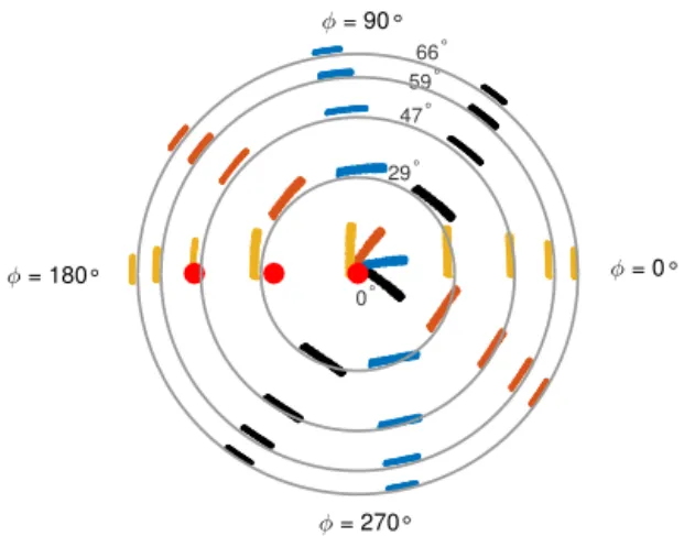
To cover a wide range of observing geometries, a total of nine scenarios based on the AirMSPI USC_SeaPRISM viewing geometry is used, as illus-trated in Fig. 2: the Sun is placed at the original inci-dence angleθ0=49.1◦as well as at 25◦and overhead

Sun (θ0=0◦). Relative azimuth angles of φ≈50, 95,

140, and 176◦are also modeled. The latter case includes glint. For the case with overhead Sun, only one azimuth angle is necessary.

2. Random noise was added to the simulated radiance and DoLP values. This is a commonly adopted measure to test the impact of measurement errors on retrieval al-gorithm performance (Dubovik et al., 2011; Hasekamp and Landgraf, 2005, 2007). We added a relative mea-surement uncertainty ofσL= ±1 % to the radiances and

an absolute uncertainty ofδDoLP= ±0.005 to the DoLP.

After a random-error test, an extra±4 % systematic er-ror was added to study the influence of calibration bias. 3. Retrieved aerosol properties and Chla concentrations

were compared to their known (input truth) values.

4.1.1 Influence of aerosol loading and absorption on nLw retrieval

As an example, we use one of the simulated scenarios of AirMSPI observation over USC_SeaPRISM AERONET-OC site (θ0=25◦, φ≈95◦) as input. Figures 3–6 compare

(11)

Table 3.Cases for truth-in/truth-out retrieval tests.

Weakly absorbing aerosol Moderately absorbing aerosol Dust aerosol

Targeted AOT at 555 nm 0.02, 0.1, 0.3, 0.5, 1.0

Aerosol

Volume fractions (fv,1–5) 4, 32, 20, 4, 40 % 16, 56, 6, 6, 16 % 2, 8, 1, 24, 65 %

Mean height of aerosol 1

distribution profile (ha, km)

Half width of aerosol 0.75 distribution profile (σa, km)

Refractive index 1.388a 1.522a 1.497

(mean of real partnr(λ))

Refractive index 1.98_×10−3a 1.32_×10−2a b (mean of imag. part:ni(λ))

Chlorophylla([Chl_a], mg m−3) 0.05, 0.2, 1.0

Surf

ace Adjustment term corresponding to±10 % perturbation on bio-optical model simulated nLw

(1aWL(λ), mW cm−2sr−1µm−1) at AirMSPI 355, 385, 445, 475, and 550, 660 and 865 nm spectral bands

Surface wind speed (W, m s−1) 4

a_{slightly dependent on wavelength but average values are listed here;}b_8.04_×₁₀−3_{(355 nm), 7.74}_×₁₀−3_{(380 nm), 4.98}_×₁₀−3_{(445 nm), 4.10}_×₁₀−3 (470 nm), 2.01×10−3(555 nm), 4.28×10−4(660 nm), and 3.27×10−4(865 nm).

0° 29°

47° 59°

66°

φ = 180° φ = 0°

φ = 270° φ = 90°

Figure 2.Simulation geometries based on AirMSPI observations over the AERONET OC-site USC_SeaPRISM on 6 February 2013. The three red dots indicate the Sun’s locationθ₀₌49.1◦, the actual value at the time of the AirMSPI overflight, as well as 25 and 0◦. For each incidence angle, four viewing geometries corresponding to the azimuthal angles_≈50, 95, 140, and 176◦are simulated, which are marked in different colors: black, blue, dark red, and dark yellow, respectively. Due to symmetry, only one azimuthal plane is neces-sary to simulate for zenith Sun location. Therefore totally nine ge-ometries are created for truth-in/truth-out test. The viewing angles corresponding to the 9 AirMSPI images form line segments. Each line segment is composed of densely sampled cross-track positions contributed by all patches in the image. For each azimuthal case, a total of nine segments are plotted.

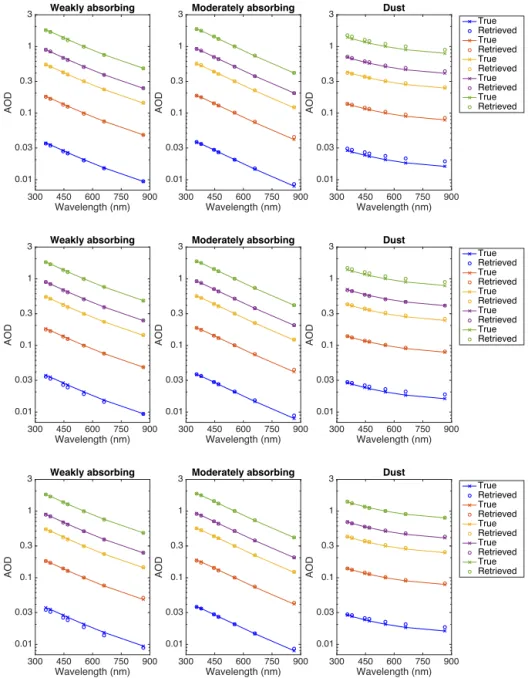
respectively, to the “true” values used in the simulation. In all figures, the top, middle, and bottom rows of the panels cor-respond to Chlaconcentrations of 0.05, 0.2, and 1 mg m−3_,

respectively (with±10 % perturbation on water-leaving radi-ances in different bands). The left, middle, and right panels correspond to weakly absorbing, moderately absorbing, and dust aerosols, respectively.

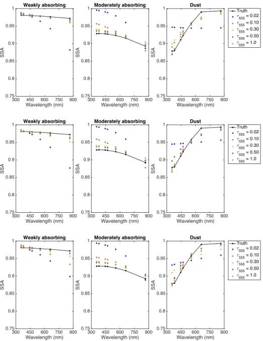
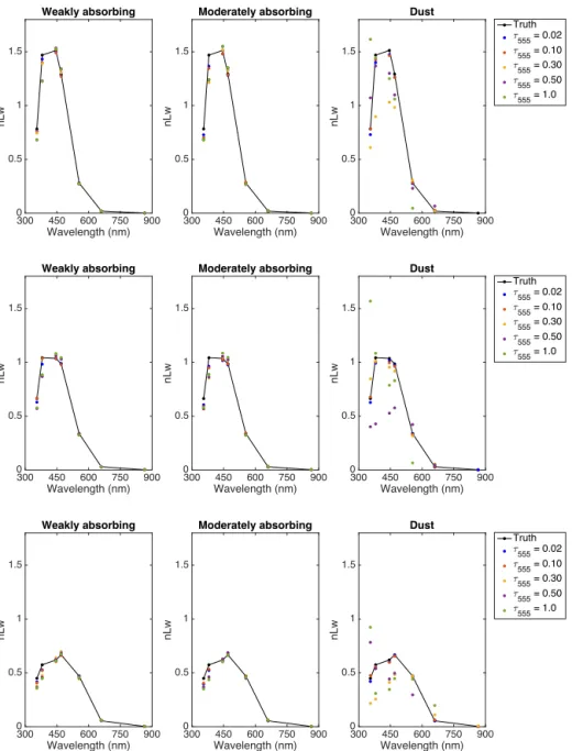
For all aerosol types, the shapes of AOD, SSA, and nLw, as a function of wavelength and PSD as a function of par-ticle radius, are similar to their true values. Due to the lim-ited contribution of nLw to TOA radiance, the aerosol re-trieval accuracy is not significantly affected by the Chl a concentration within the range modeled here. The retrievals over dust are less accurate than for the weakly and moder-ately absorbing aerosols, due to the fact that dust aerosols are dominated by coarse-mode particles and the extinction is more spectrally neutral, so the information provided by the multispectral measurements between 355 and 865 nm is less effective to constrain the aerosol retrieval. As ex-pected, Fig. 6 shows higher retrieved nLw accuracy at low AOD loading (τ555≤0.1) due to greater atmospheric

(12)

water-leaving radiance. As AOD and SSA errors are the largest for dust aerosols, the normalized water-leaving radiance retrieval error also becomes largest in the presence of dust.

A more comprehensive view of aerosol retrieval errors is displayed in Fig. 7a–d. Though the absolute error of re-trieved AOD increases as the aerosol loading increases (see Fig. 7a), the relative error of AOD (100× |AODretrieved−

AODtrue|/AODtrue) generally decreases as the TOA

radi-ance carries more aerosol information at higher loading (see Fig. 7b). For the same reason, an inverse relationship be-tween aerosol loading and absolute error in single-scattering albedo (|SSAretrieved−SSAtrue|) is observed, as shown in

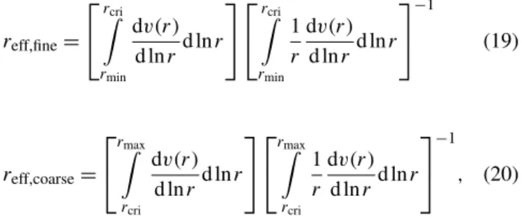
Fig. 7c. To evaluate the retrieval error for size distribution, the effective radius is used and calculated for fine and coarse modes:

reff,fine=

 

rcri Z

rmin

dv(r) d lnrd lnr

   

rcri Z

rmin

1 r

dv(r) d lnrd lnr

 

−1

(19)

reff,coarse=

 

rmax_Z

rcri

dv(r) d lnrd lnr

 

 

rmax_Z

rcri

1 r

dv(r) d lnrd lnr

 

−1 , (20)

where the lower size limitrmin=0.04 µm and the upper size

limitrmax=15 µm. Settingrcrito be 0.75 µm for weakly and

moderately absorbing aerosols andrcrito be 0.25 µm for dust

aerosols to distinguish fine and coarse modes, a generally in-verse relationship between aerosol loading and the relative error in effective radius of fine and coarse-mode aerosols (100× |reff, retrieved−reff, true|/reff, true)is also observed for

all types of aerosols, as shown in Fig. 7d. Forτ555≥0.3, the

maximum retrieval error in AOD is ∼2.5, 2.5, and 7 % for weakly, moderately absorbing aerosols, and dust particles, respectively. The maximum retrieval error for SSAω0,355 nm

is ∼0.005, 0.015, and 0.025 for weakly absorbing, moder-ately absorbing, and dust aerosols, respectively. We find that the maximum error in SSA for the weakly absorbing aerosol appears at red and near-infrared bands (660 and 865 nm) for all aerosol loading cases, suggesting that there is less sensi-tivity to SSA as the ocean reflectance decreases. For the mod-erately absorbing aerosols, the maximum error is observed at the two UV bands (355 and 385 nm), indicating higher er-rors as absorption increases, particularly at low aerosol load-ing. Moreover, increasing AOD is found to be helpful for constraining the SSA retrieval for both weakly and moder-ately aerosols. However, for dust aerosols, where SSA spans a larger range as a function of wavelength compared to the weakly and moderately absorbing aerosols, limited improve-ment on SSA retrieval accuracy is gained by increasing AOD. Figure 7d shows that for weakly and moderately absorb-ing aerosols the effective radius for coarse-mode aerosols has larger retrieval errors than the fine mode aerosol. We attribute this to the fact that the longest spectral band of AirMSPI used

in the retrievals (865 nm) is insufficient to fully constrain the coarse-mode aerosol PSD.

In Fig. 7e–f, which correspond to Chla concentration to be 0.05, 0.2, and 1.0 mg m−3(with±10 % perturbation im-posed on the water-leaving radiance), the retrieval error of normalized water-leaving radiance (1nLw=nLwretrieved−

nLwtrue)is plotted against uncertainty metrics specified by

the PACE Science Definition Team (SDT) (Del Castillo et al., 2012), i.e., a relative error of 5 % or an absolute error of 0.001×F0/π (whichever is larger) in the visible, and twice

these values in the UV. For weakly and moderately absorb-ing aerosols, the accuracy of nLw at all visible bands mostly falls within the PACE SDT requirement for all aerosol load-ings and Chla concentrations. The uncertainty in retrieved nLw in the pair of UV bands, however, falls outside the spec-ified bounds whenτ555>∼0.1. As the TOA signals in the

UV are dominated by Rayleigh scattering, accurate retrieval of water-leaving radiance remains challenging even after the interpatch smoothness constraints on aerosol variation and spectral smoothness constraints on aerosol optical properties are imposed. For all Chlaconcentrations, errors in nLw are largest for dust aerosols, and fall outside the PACE SDT re-quirement forτ555>∼0.1, even in the visible. These errors

can potentially be reduced if an improved bio-optical model can be devised that relates the more accurately determined visible nLw values to the values in the UV.

Figure 7 shows that for all aerosol types, even though the retrieval errors of SSA and AOD at low aerosol loading (τ555<0.1) are relatively larger than at high AOD, these

er-rors do not propagate to the retrieval of nLw. This is because in the single-scattering regime, the path radiance is domi-nated by scattering optical depth, which is the product of AOD and SSA. This means AOD and SSA errors counter-act each other to some extent (i.e., an overestimated AOD is compensated by an underestimated SSA and vice versa) so that scattering optical depth is less biased, leading to a re-duced impact on the retrieval of nLw. However, when AOD increases, the fraction of water-leaving radiance in the TOA signal reduces significantly, and accurate separation of its weak contribution in the multiple-scattering regime becomes more difficult. The presence of dust aerosols further compli-cates the retrievals as the aerosols and CDOM share a similar shape of absorption spectra, namely, increasing absorption at shorter wavelengths (Aurin and Dierssen, 2012; Bergstrom et al., 2007).

4.1.2 Effect of multipatch vs. single-patch retrieval Taking the case of median loading (τ555=0.3) of

(13)

300 450 600 750 900 Wavelength (nm) 0.01

0.03 0.1 0.3 1 3

AOD

Weakly absorbing

300 450 600 750 900

Wavelength (nm) 0.01

0.03 0.1 0.3 1 3

AOD

Moderately absorbing

300 450 600 750 900

0.03 0.1 0.3 1 3

AOD

Dust

True Retrieved True Retrieved True Retrieved True Retrieved True Retrieved

300 450 600 750 900 Wavelength (nm) 0.01

0.03 0.1 0.3 1 3

AOD

300 450 600 750 900 Wavelength (nm) 0.01

0.03 0.1 0.3 1 3

AOD

300 450 600 750 900 Wavelength (nm) 0.01

0.03 0.1 0.3 1 3

AOD

Dust

300 450 600 750 900 Wavelength (nm) 0.01

0.03 0.1 0.3 1 3

AOD

300 450 600 750 900 Wavelength (nm) 0.01

0.03 0.1 0.3 1 3

AOD

300 450 600 750 900 Wavelength (nm) 0.01

0.03 0.1 0.3 1 3

AOD

Dust

Figure 3.Simulated true and retrieved spectral AOD for different scene conditions. Left column of three panels: weakly absorbing aerosol. Middle column of three panels: moderately absorbing aerosol. Right column of three panels: dust aerosol. AOD is retrieved for three values of Chlaconcentration: 0.05 (top row of panels), 0.2 (middle row of panels), and 1.0 mg m−3(bottom row of panels), with_±10 % perturbation of water-leaving radiance. Five aerosol loadings, corresponding toτ555=0.02, 0.10, 0.30, 0.50, and 1.0, are plotted in dark blue, dark red,

dark yellow, purple, and green, respectively. The lines with crosses at the AirMSPI wavelengths represent the true AODs, while the open circles correspond to the retrieved values. The synthetic data are from one of the simulated scenarios of AirMSPI observation over USC_ SeaPRISM AERONET-OC site (θ0=25◦,φ≈95◦). Though not plotted, the spatial variation of the retrieved AOD across the whole image

is less than 1 % for all spectral bands.

is used. While the single patch-based retrieval leads to spa-tially highly variable Chlaconcentrations with a mean value of 0.26 mg m−3 (namely 30 % retrieval error), the multi-patch algorithm yields a more stable and accurate value of 0.21 mg m−3, which is within 5 % of the true value. Cor-respondingly, the accuracy of the nLw retrieval improves by 0.04, 0.03, and 0.01 mW cm−2sr−1µm−1 at 445, 470,

(14)

ob-300 450 600 750 900 Wavelength (nm) 0.75

0.8 0.85 0.9 0.95 1

SSA

300 450 600 750 900 Wavelength (nm) 0.75

0.8 0.85 0.9 0.95 1

SSA

300 450 600 750 900 Wavelength (nm) 0.75

0.8 0.85 0.9 0.95 1

SSA

Dust

Truth =

555 = 0.02 =

555 = 0.10 =

555 = 0.30 =

555 = 0.50 =

555 = 1.0

300 450 600 750 900 Wavelength (nm) 0.75

0.8 0.85 0.9 0.95 1

SSA

300 450 600 750 900 Wavelength (nm) 0.75

0.8 0.85 0.9 0.95 1

SSA

300 450 600 750 900 Wavelength (nm) 0.75

0.8 0.85 0.9 0.95 1

SSA

Dust

Truth =

555 = 0.02 =

555 = 0.10 =

555 = 0.30 =

555 = 0.50 =

555 = 1.0

300 450 600 750 900

0.8 0.85 0.9 0.95 1

SSA

300 450 600 750 900

0.8 0.85 0.9 0.95 1

SSA

300 450 600 750 900

0.8 0.85 0.9 0.95 1

SSA

Dust

Truth =

555 = 0.02 =

555 = 0.10 =

555 = 0.30 =

555 = 0.50 =

555 = 1.0

Figure 4.Panel layout as in Fig. 3 but for retrieved single-scattering albedo. The black line with dots placed at the AirMSPI wavelengths represents the true SSA. The colored symbols represent retrieved SSA for various values of AOD.

servation are highly nonunique subjected to local optimum solutions. Through the imposition of interpatch smoothness constraints on aerosol loading and Chl a concentration, the multipatch retrieval yields results that are closer to the truth. As indicated in Fig. 8b, the multipatch algorithm also shows greater noise resistance in all three quantities (nLw, AOD and SSA) simultaneously. The AOD error in the single-patch re-trieval decreases as the level of random noise in intensity increases from 0.5 to 2.0 %, due to that fact that the errors mainly propagate into nLw and SSA.

4.1.3 Comparison to direct water-leaving radiance retrieval

(15)

re-0.01 0.1 1 10 100 Radius (7m) 0 0.1 0.2 0.3 0.4 0.5 0.6 dv/dln(r) Weakly absorbing

0.01 0.1 1 10 100 Radius (7m) 0 0.1 0.2 0.3 0.4 0.5 0.6 0.7 0.8 0.9 dv/dln(r) Moderately absorbing

0.01 0.1 1 10 100 Radius (7m) 0 0.1 0.2 0.3 0.4 0.5 0.6 dv/dln(r) Dust Truth =

555 = 0.02 =

555 = 0.10 =

555 = 0.30 =

555 = 0.50 =

555 = 1.0

0.01 0.1 1 10 100

Radius (7m)

0 0.05 0.1 0.15 0.2 0.25 0.3 0.35 0.4 0.45 0.5 dv/dln(r) Weakly absorbing

0.01 0.1 1 10 100

Radius (7m)

0 0.1 0.2 0.3 0.4 0.5 0.6 0.7 0.8 dv/dln(r) Moderately absorbing

0.01 0.1 1 10 100

Radius (7m)

0 0.1 0.2 0.3 0.4 0.5 0.6 dv/dln(r) Dust Truth =

555 = 0.02

=

555 = 0.10

=

555 = 0.30

=

555 = 0.50

=

555 = 1.0

0.01 0.1 1 10 100 Radius (7m) 0 0.1 0.2 0.3 0.4 0.5 0.6 dv/dln(r) Weakly absorbing

0.01 0.1 1 10 100 Radius (7m) 0 0.1 0.2 0.3 0.4 0.5 0.6 0.7 0.8 0.9 dv/dln(r) Moderately absorbing

0.01 0.1 1 10 100 Radius (7m) 0 0.1 0.2 0.3 0.4 0.5 0.6 dv/dln(r) Dust Truth =

555 = 0.02 =

555 = 0.10 =

555 = 0.30 =

555 = 0.50 =

555 = 1.0

Figure 5.Panel layout as in Fig. 3 but for retrieved normalized aerosol size distribution. The black lines correspond to the true size distribu-tion, with dots at discrete values of particle radius. The colored lines represent retrieved size distributions for various values of AOD.

trieval accuracy improves by 0.01 and 0.02 at 350 and 865 nm, respectively. Moreover, a remarkable gain in nLw accuracy by about 6, 11, and 12 %, or 0.07, 0.12, and 0.03 mW cm−2sr−1µm−1in absolute magnitude at 445, 470, 555 nm, respectively, is achieved when the bio-optical model is used. Given that the PACE SDT specification tolerates an uncertainty of ∼0.06 mW cm−2sr−1µm−1 in these bands, the accuracy gain from using the bio-optical model is sig-nificant.

4.1.4 Influence of systematic error

(16)

300 450 600 750 900

Wavelength (nm)

0 0.5 1 1.5

nLw

300 450 600 750 900

Wavelength (nm)

0 0.5 1 1.5

nLw

300 450 600 750 900

Wavelength (nm)

0 0.5 1 1.5

nLw

Dust

Truth =

555 = 0.02

=₅₅₅ = 0.10

=₅₅₅ = 0.30

=

555 = 0.50

=

555 = 1.0

300 450 600 750 900

Wavelength (nm) 0

0.5 1 1.5

nLw

300 450 600 750 900

Wavelength (nm) 0

0.5 1 1.5

nLw

300 450 600 750 900

Wavelength (nm) 0

0.5 1 1.5

nLw

Dust

Truth =

555 = 0.02

=

555 = 0.10

=₅₅₅ = 0.30

=

555 = 0.50

=

555 = 1.0

300 450 600 750 900

Wavelength (nm)

0 0.5 1 1.5

nLw

300 450 600 750 900

Wavelength (nm)

0 0.5 1 1.5

nLw

300 450 600 750 900

Wavelength (nm)

0 0.5 1 1.5

nLw

Dust

Truth =₅₅₅ = 0.02 =

555 = 0.10

=

555 = 0.30

=

555 = 0.50

=

555 = 1.0

Figure 6.Panel layout as in Fig. 3 but for retrieved values of nLw (mW cm−2sr−1µm−1). The black lines correspond to the true nLw, with dots placed at the AirMSPI wavelengths. The colored symbols represent retrieved nLw for various values of AOD.

errors and random noise. To model its effect, we keep the random noise levels used in the previous analysis and add a ±4 % systematic error to the simulated radiance signals. The resulting retrieval errors of AOD, SSA, effective radii of fine- and coarse-mode aerosol, nLw, and band-to-band ratio are displayed in Fig. 10a–f, respectively.

Comparison of Figs. 7 and 10 shows that systematic er-rors have a larger impact on retrieval accuracy than random errors, as the latter are suppressed by using a lot of patches for retrieval while the former are not. For AOD and SSA, a negative radiance bias causes larger retrieval errors than a positive bias. Comparison of Figs. 10e and 7e shows that er-rors in nLw due to an intensity bias increase at all AODs:

at low aerosol loading the errors propagate to nLw while at high loading the contribution of nLw to the TOA signal is weak, exacerbating errors. On the other hand, comparison of Figs. 10f with 7h shows a much smaller effect of system-atic errors on1nLw(λ)/nLw(555); in other words, the sys-tematic errors mainly propagate to the overall magnitude of nLw(λ)curve while the relative spectral shape is affected to a much lesser degree.

4.2 Retrievals with real AirMSPI observations

(17)

ob-Figure 7.

servations acquired over the USC_SeaPRISM AERONET-OC site and near the AERONET site in La Jolla. The USC_SeaPRISM and La_Jolla scenes were chosen from a larger set of AirMSPI field campaign images to ensure cloud free conditions. The data were processed with the recently upgraded data processing pipeline, which includes vicarious radiometric calibrations and improved polarimetric calibra-tion making use of onboard polarizacalibra-tion sources. Nadir inten-sity and DoLP images from combinations of different spec-tral bands for these two target areas are shown in Figs. 11a and 12a. Maps of retrieved AOD and SSA at 555 nm, nLw at 445 and 555 nm spectral bands are displayed in Figs. 11b and 12b.

Selecting the image patch that is closest to the AERONET site, our retrieved AOD, SSA, size distribution, and nLw are compared to the independent AERONET results, as shown in Figs. 11c and 12c. We first discuss results from the USC_SeaPRISM retrievals. The AERONET site re-ported a relatively high 550 nm AOD of 0.30 and 0.26 at 19:08 and 20:08 UTC, respectively, and our retrieval returns an intermediate value of 0.27 from the AirMSPI data ac-quired at 19:40 UTC. The differences between the AirM-SPI and AERONET AOD and SSA retrievals are within the

Figure 7.

AERONET SSA retrieval uncertainties (e.g., 0.015 forτ440

and 0.03 forω0,440atτ440> 0.2, see Table 4 of Dubovik et

al., 2000). The Generalized Retrieval of Aerosol and Sur-face Properties (GRASP) algorithm by Dubovik et al. (2011, 2014) was also run, and the difference between the GRASP and JPL algorithms is on the order of∼0.025 for AOD and

∼0.008 for SSA in all bands.

(18)

Figure 7.

the differences are found to be 0.0396, 0.0118, 0.0198, and 0.0077 mW cm−2sr−1µm−1 in the 445, 470, 555, and 660 nm bands, respectively. These differences are within the AERONET-OC uncertainties of 0.0462, 0.0516, 0.0279, and 0.0167 mW cm−2sr−1µm−1in the four bands, obtained by interpolating combined standard uncertainties in validated nLw at various AERONET-OC sites (Gergely and Zibordi, 2014). Note that the nonspherical particle fraction retrieved using both GRASP and JPL algorithm is negligible and the results are not displayed here.

For the second study site, the AirMSPI target area was about 13 km away from the La Jolla AERONET station. In spite of the distance, the differences between the AirM-SPI and AERONET AOD and SSA values are both within AERONET’s uncertainty, as observed from the upper two plots of Fig. 12c. Though the difference in PSD in some size bins falls outside the AERONET uncertainty range, the bimodality of the size distribution is identified even at the low aerosol loading for this case (τ555∼0.04). Independent

Figure 7.Retrieval errors of(a)AOD; (b)AOD (relative differ-ence);(c)SSA;(d)effective radii for fine and coarse-mode aerosols;

(e)–(g)nLw (signed difference) corresponding to Chla concentra-tions 0.2, 0.05 and 1.0 mg m−3, respectively (with_±10 % pertur-bation imposed on the water-leaving radiance); and(h) band ra-tios (Rλ, nLw₌nLw(λ)/nLw(555)). The retrieval errors of aerosol properties show similar features for all Chlaconcentrations. There-fore the results corresponding to [Chl_a]₌0.2 mg m−3 are dis-played in(a)–(d). Via truth-in/truth-out tests, the uncertainties are estimated for AirMSPI multispectral, multiangular, and multipolari-metric observations over a 5 km_×5 km ocean area. The simulation is based on nine combinations of Sun incidence and viewing ge-ometries. Relative random noise of 1.0 % is used for radiance and absolute random noise of 0.005 is used for DoLP. The colors cor-respond to seven different AirMSPI spectral bands. The maximum water-leaving radiance error target specified by the PACE Science Definition Team (SDT) is plotted as black curves. The uncertainty of nLw at 865 nm is not displayed since the PACE SDT did not spec-ify a requirement on this band. The spread of the error, depicted by the vertical bars, reflects the dependence on illumination and view-ing geometries.

surface measurements to validate the nLw retrieval were not available at this site.

5 Summary and outlook

(19)

(a)

(b) Wavelength (nm)

300 450 600 750 900

AOD 0.1 0.2 0.3 0.4 0.5 0.6 Wavelength (nm)

300 450 600 750 900

SSA 0.75 0.8 0.85 0.9 0.95 1 Truth Multipatch retrieval Single-patch retrieval

Radius (7m) 0.01 0.1 1 10 100

dv/dln(r) 0 0.01 0.02 0.03 0.04 0.05 Patch no.

20 40 60 80 100

[Chl a ] (mg m ) 3 0.15 0.2 0.25 0.3 0.35 0.4 0.45

Random error (%)

0 1 2 3

" nLw 0 0.1 0.2 Multipatch retrieval 355 nm 385 nm 445 nm 470 nm 555 nm 660 nm 865 nm

Random error (%)

0 1 2 3

" nLw 0 0.1 0.2 Single-patch retrieval

Random error (%)

0 1 2 3

"

AOD

0 0.02 0.04

Random error (%)

0 1 2 3

"

AOD

0 0.02 0.04

Random error (%)

0 1 2 3

"

SSA

0 0.025 0.05

Random error (%)

0 1 2 3

" SSA 0 0.025 0.05 –

Figure 8. Comparison of single-patch- and multipatch-based re-trievals of(a)AOD, SSA, aerosol size distribution, and Chla con-centration for the median AOD (τ555=0.3) of weakly absorbing

aerosols and Chl aconcentration of 0.2 mg m−3. The simulation uses the Sun and viewing geometry corresponding to the AirMSPI overflight of the USC_ PRISM AERONET site. Image-averaged Chlaconcentrations are 0.29 and 0.22 mg m−3for the single- and multipatch-based retrievals, respectively. A random error of 1.0 % and 0.005 is added to the simulated intensity and DoLP data, respec-tively;(b)AOD, SSA, and nLw (mW cm−2sr−1µm−1) retrieved with different levels of random noise (0.5, 1.0, 2.0, and 3.0 %) added to the simulated BRF while the noise in DoLP is kept at 0.005. The aerosol loading, Chlaconcentration, and Sun and viewing geome-try are the same as in Fig. 8a.

imaginary parts of aerosol refractive index, aerosol concen-trations of different size components, mean height and width of aerosol distribution, nonspherical particle fraction, wind speed over ocean surface, and normalized water-leaving ra-diance. An efficient RT modeling strategy has been devel-oped that couples separate runs for modeling RT in two Rayleigh layers, an aerosol/Rayleigh mixed layer, and an ocean medium. Repeated, time-consuming RT computations for layers whose properties are not perturbed during

Jaco-Wavelength (nm)

300 450 600 750 900

AOD 0.1 0.2 0.3 0.4 0.5 0.6 Wavelength (nm)

300 450 600 750 900

SSA 0.75 0.8 0.85 0.9 0.95 1 Truth Bio-optical model Lambertian model

Radius (7m)

0.01 0.1 1 10 100

dv/dln(r) 0 0.01 0.02 0.03 0.04 0.05 Wavelength (nm)

300 450 600 750 900

n L w ( m W c m -s r-u m ) 2 0 0.3 0.6 0.9 1.2 –

Figure 9.AOD, SSA, aerosol size distribution, and nLw retrieved using the bio-optical model compared to retrievals in which water-leaving radiance is modeled simply as Lambertian with arbitrary albedo.

Figure 10.