Bifurcation analysis of a paradigmatic model of monsoon prediction

SRef-ID: 1607-7946/npg/2005-12-707 European Geosciences Union

© 2005 Author(s). This work is licensed under a Creative Commons License.

Nonlinear Processes

in Geophysics

Bifurcation analysis of a paradigmatic model of monsoon prediction

A. Kumar Mittal1,2,3, S. Dwivedi1,2,3, and A. Chandra Pandey1,2,3

1_{M. N. Saha Centre of Space Studies, Institute of Interdisciplinary Studies, University of Allahabad, Allahabad, India} 2_{K. Banerjee Centre of Atmospheric and Ocean Studies, Institute of Interdisciplinary Studies, University of Allahabad,}

Allahabad, India

3_{Department of Physics, University of Allahabad, Allahabad, India}

Received: 28 October 2004 – Revised: 15 June 2005 – Accepted: 16 June 2005 – Published: 18 July 2005

Abstract. Local and global bifurcation structure of the

forced Lorenz model in ther−F plane is investigated. The forced Lorenz model is a conceptual model for understanding the influence of the slowly varying boundary forcing like Sea Surface Temperature (SST) on the Indian summer monsoon rainfall variability. Shift in the probability density function between the two branches of the Lorenz attractor as a func-tion of SST forcing is calculated. It is found that the one-dimensional return map (cusp map) splits into two cusps on introduction of forcing.

1 Introduction

Rainfall over India varies both in space and time during the Summer monsoon season and the large-scale rainfall oscil-lates aperiodically between active spells with good rainfall and weak spells with little rainfall. Typically the transition time between active and weak spells is shorter than the res-idence time (few weeks) of the spells themselves. Rama-murthy (1969) and Sikka and Gadgil (1980) conducted an exhaustive analysis of the daily rainfall over India and re-lated the active/break periods to location of monsoon trough. Although rainfall is one of the most highly variable quanti-ties, both in observations and in model simulations, seasonal mean rainfall anomalies are largely determined by the sea surface temperature (SST) (Shukla, 1998). The influence of the slowly varying boundary forcing like SST is to bias the system towards more active/break regimes thus altering the shape of the probability density function.

Because of the interaction between atmosphere and ocean, the SST of the Indian and Pacific Oceans may influence the variability of the Indian monsoon and in turn, the monsoon winds and rainfall may affect the variability of the SST of the referred oceans. This mutual interaction introduces the possibility that the monsoon and the oceans form a coupled

Correspondence to:S. Dwivedi (suneetdwivedi@yahoo.co.in)

climatic system (Webster and Yang, 1992). However, the In-dian monsoon rainfall is understood to have a stronger rela-tion with the Pacific Ocean SST than with the Indian Ocean SST.

The lower boundary conditions like SST are less chaotic and therefore can lend partial predictability to the atmo-sphere. Charney and Shukla (1981) proposed that the sea-sonal monsoon rainfall over India although being one of the most highly variable quantities, has potential predictability, because it is forced by the slowly varying boundary condi-tions such as sea surface temperature (SST), soil moisture, sea ice and snow. There are several studies, both observa-tional and modelling indicating that the interannual variabil-ity of Indian summer monsoon (JJAS) rainfall is linked to the SST variation in Pacific (Rasmusson and Carpender, 1983; Mooley and Parthasarathy, 1983; Ju and Slingo, 1995; So-man and Slingo, 1997). The SST has a strong influence on atmospheric dynamics, while it itself remains coherent over large spatial scales. It varies slowly on time-scales of individ-ual weather events, but it is not constant from year to year. In particular, it is known that year-to-year variations in tropical Pacific SST associated with the El Nino/Southern oscillation event have a strong influence on the inter-annual variations in the monsoon.

The monsoon region has a dominant intraseasonal fluctua-tion with periodicity of 30–50 days (Sikka and Gadgil, 1980; Yasunari, 1980; Krishnamurthy and Sybramaniyam, 1982). Large-scale rainfall over the Indian region is associated with the so-called “Inter-tropical convergence zone” (ITCZ), a re-gion where lower tropospheric winds are convergent. For In-dian longitudes, ITCZ may be located over the heated conti-nent, leading to active monsoon phase, or over the equatorial Indian Ocean, leading to break phase.

It has been shown by Sikka and Gadgil (1980) that the probability distribution function of the ITCZ is bimodal. To be specific, one may assume that the positive x-y regime in the Lorenz attractor corresponds to the oceanic ITCZ with reduced monsoon rainfall, and that the negative x-y regime corresponds to the continental ITCZ with the enhanced mon-soon rainfall.

Motivated by the above observations, Palmer (1994) intro-duced constant “forcing” terms in the Lorenz (1963) equa-tions to put forward a paradigmatic model for discussing long-range monsoon predictability. In this model, the “forc-ing” terms correspond to the tropical Pacific SST anomaly. The two branches of the forced Lorenz attractor correspond to the two regimes of active and weak spells of the monsoon. In the absence of forcing, both the branches are equally likely. When forcing is introduced, the probability of the state lying in one of the branches is greater than that in the other branch. Palmer (1994) has hypothesised that slowly varying boundary conditions change only the nature of the intraseasonal variability. He suggested that Summer mon-soon evolves nonperiodically between the regimes of active and the break phases. The seasonal mean rainfall is deter-mined by the bimodal probability distribution function (PDF) of rainfall, depending on the frequency and length of active and break periods. The spatial patterns of the interannual variability of the monsoon rainfall, for example, should cor-respond to those of intraseasonal active and break periods. In an evaluation of NCEP-NCAR reanalysis circulation data, Goswami and Ajaya Mohan (2001) lend support to Palmer’s hypothesis by identifying a mode of variability common to both intraseasonal and interannual time scales and an asym-metric bimodal PDF of active and break conditions.

The forced Lorenz model has been the subject of various studies (Pal, 1996; Pal and Shah, 1999; Mehta et al., 2003; Mittal et al., 2003).

In recent years bifurcation analysis has proven to be an important tool for mathematical analysis and better under-standing of the internal dynamics and physics of low order ocean atmospheric models. There are several parameters in the atmosphere and ocean which, when changing beyond a critical value, lead to entire changes of the nature of the sys-tem. The need therefore is to identify such parameters and to see how they are affecting the atmosphere when they pass beyond a critical value.

Regular and chaotic behaviour in the Lorenz-84 model, which is a low order general circulation model of the atmo-sphere (Lorenz, 1984, 1987, 1990) has been studied exten-sively using bifurcation theory by Masoller et al. (1992) and Sicardi Schifino and Masoller (1996). Masoller et al. (1995) have investigated the dynamics of the Lorenz-84 model of general circulation of the atmosphere by full characterisation of chaotic strange attractors found. A comprehensive bifur-cation and predictability analysis of the Lorenz-84 model has been done by Shil’nikov, Nicolis and Nicolis (1995). Roeb-ber (1995) has investigated the dynamical behaviour of the climate system using a low order coupled atmosphere-ocean general circulation model, in order to gain some qualitative

understanding of how nonlinear interactions between the in-dividual system components may affect the climate. Van Veen (2001) has done a detailed study of the baroclinic flow and the Lorenz-84 model.

These studies motivated us to present a mathematical anal-ysis of the forced Lorenz model. We have done the analanal-ysis first by varying the forcing along two particular lines in the Fx−Fyplane and then by also varyingralong with the forc-ing F. We have investigated the local and global bifurca-tion structure of the forced Lorenz model in ther−F plane, whereF parameterises a particular line in theFx−Fyplane. We also study the shift in the probability density function be-tween the two branches of the Lorenz attractor as the forcing (anomalous SST) is changed. We found that by introducing the forcing term, the one-dimensional return map (cusp map) produced by the maximumzvalues splits into two cusps.

2 Bifurcation analysis of the forced Lorenz model

The system of equations for the forced Lorenz model is: dx

dt = −ax+ay+cFx

dy

dt = −xz+rx−y+cFy

dz

dt =xy−bz+cFz, (1) wherea=10,b=8/3 andr=28.

The (x, y, z)→(−x, −y, z) symmetry of the original Lorenz equations (Lorenz, 1963) is lost in the forced Lorenz system.

The transformationz=z′+ c_bFz; r=r′+ _bcFz clearly tells us that the forcingFzis equivalent to a shift in the pa-rameterr. Therefore, without loss of generality we study the system

dx

dt = −ax+ay+Fx

dy

dt = −xz+rx −y+Fy

dz

dt =xy−bz . (2)

To make the analysis simpler we study here two particularly simple cases:

Case I:Fx=aF, Fy=−F and case II:Fx=aF, Fy=−rF. In case I, ifF2<4b(1-r)there is only one fixed pointO (0,−F, 0). ForF2>4b(1-r)there are two more fixed points P±(x±, y±, r−1), where

x±= 1 2

F±

q

F2_+4b(r−1)

and y±=

1 2

−F±

q

F2_+4b(r−1)

P

P

F

= 0

y

x

_z

(a)

x

_z

P

P

F

=

−

1

(b)

y

y

F

=

−

0. 15

z

x

P

P

(c)

y

Fig. 1. Fixed pointsP+andP−for a=10, b=8/3,r=28(a)F=0,

P+=(8.4853,8.4853,27) andP−=(−8.4853,−8.4853,27);(b)case

I,Fx=aF, Fy=−F, P+=(8, 9, 27) andP−=(−9, −8, 27); and (c)case II,Fx=aF,F y=−rF,P+=(8.4853, 8.6353, 27.4773) and

P−=(−8.4853,−8.3353, 26.5227).

The fixed pointsP+/P− represent a state of continuous rainfall/complete absence of rainfall. They are shown in Fig. 1a for no forcing i.e.F=0, in Fig. 1b for the case I with F=−1, and in Fig. 1c for case II withF=−0.15.

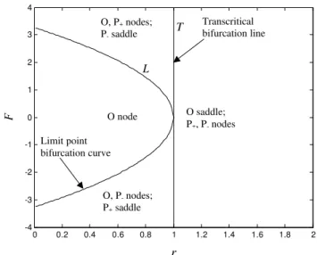
0 0.2 0.4 0.6 0.8 1 1.2 1.4 1.6 1.8 2 -4

-3 -2 -1 0 1 2 3 4

r

F

L T

O node

O, P+ nodes;

P- saddle

O, P- nodes;

P+ saddle

O saddle;

P+, P- nodes

Limit point bifurcation curve

Transcritical bifurcation line

Fig. 2.Bifurcation structure of the forced Lorenz Model in case I, i.e.Fx=aF,Fy=−Faroundr=1.

For the case I, the eigenvalues of the linear tangent model matrix at the fixed pointOare:

−band

−(a+1)± q

(a+1)2_−4a(1−r)

/2.

Forr<1, all the eigenvalues are negative andO is a stable node. One of the eigenvalues is positive forr>1. Hence, for r>1,Ois an unstable fixed point. The characteristic equa-tions at the fixed pointP±are:

λ3+(a+b+1)λ2+(ab+b+x_±2)λ+a(x2_±+x±y±)=0. (4) Figure 2 shows two curves in ther−Fplane (i)Lgiven by F2=4b(1−r)and (ii)T given byr=1. For parameter points to the left ofL, there is only one fixed pointO. For the re-gion to the right ofL, there are two more fixed pointsP+and P−. Immediately to the right ofT, both these fixed points are stable nodes, whereas in the region betweenLandT, one is a stable node whereas the other is a saddle point. In this re-gion, forF >0,P+is a stable node, whereasP−is a saddle point. ForF <0, it is the other way round. We notice thatL represents a limit point bifurcation (Thompson and Stewart, 2002), where a node – saddle pair is born. ForF >0 (F <0), as T is crossed from left to right, O andP− (P+)collide and exchange their stability. Thus,T represents a transcriti-cal bifurcation (Thompson and Stewart, 2002). The curvesL andT touch at the pointr=1,F=0. For the unforced Lorenz model, this is a point of pitchfork bifurcation (Thompson and Stewart, 2002). For the two parameter bifurcation consid-ered here this point may be regarded as a codimension 2 bi-furcation point (Kuznetsov, 1998) obtained by the touching of the limit point bifurcation and the transcritical bifurcation curves.

For F=0, if a>(b+1), as r is increased beyond rc =

a (a+b+3) (a−b−1)

r Fc ( − Fc ) Fc

−Fc

r rs rc

Fig. 3.Plot ofFcvs.rfor fixed pointP+(P−) in case I, i.e.Fx=aF,

Fy=−F[P+(P−) is locally stable ifF >Fc(F <−Fc)].

We defineFcsuch that ifF >Fc,P+is stable, whereas if F <−Fc, P−is stable.

In Fig. 3,Fc is plotted as a function ofr, taking the stan-dard valuesa=10 andb=8/3, where Fc = (a−b−1)(r− rc)

b (b+1){a(r−rs)}

1/2

andrs = rc−

b+1

a

(rc−1). It is seen that for r>rc, the equilibrium point P+ (P−), which was unstable in the absence of forcing, can be made stable by a sufficiently large positive (negative) forcing parameter F. Forrs<r<rc,P+(P−), which is stable in the absence of forcing, can be made unstable by a negative (positive) forcing parameterF of sufficiently large magnitude. For 1<r<rs, the equilibrium pointsP±are stable for all values of the forc-ing parameterF.

In case II, forr<1, there is only one fixed point atO(F, 0, 0). Forr>1 there are two more fixed pointsP±(x±,y±,z±), where

x±= ± p

{b(r−1)}, y±= ± p

{b(r−1)} −F and

z±=(r−1)− ±F s _(r− 1) b ! . (5)

The characteristic equation at the fixed pointOis given by λ3+(a+b+1)λ2+ab+a+b−ar+F2λ

+ab(1−r)+aF2=0. (6)

The equilibrium point O becomes stable, if F >Fc or F <−Fc, where

F_c2=         

b(r−1) ,for 1<r<r′ maxa(r−r′), b(r−1),for r′<r<r′′ maxa(r−r′), b(r−1) ,

a(a+1)(r−r′′₎

(b+1) i

,for r>r′′

(7)

0 5 10 15 20 25 30

-30 -20 -10 0 10 20 30 L HO

T HP

Fc p c F r F

O, P- stable;

P+ unstable

O, P+ stable;

P- unstable

P- stable;

O, P+ unstable

P+ stable;

O, P- unstable

O unstable;

P+, P- stable

rc

rI

Fig. 4. Bifurcation structure of the forced Lorenz Model in case II, i.e. Fx=aF, Fy=−rF around r=rI. Here, O is locally

sta-ble ifF >Fc orF <−Fc andP+(P−) is locally stable ifF <Fcp

(F >−Fcp).

wherer′=h1+b(a_a+1)iandr′′=h1+b(a+_ab+1)i. The fixed pointOin case II becomes stable for sufficiently large values of the forcing parameter magnitude unlike the case I where the fixed pointOremains unstable forr>1.

The characteristic equations at fixed pointP± of case II are:

λ3+(a+b+1)λ2+nab+b+a(1−r+z±)+x±2 o

λ

+anb(1−r+z±)+x±2 +x±y±) o

=0. (8)

Necessary and sufficient condition for all roots of the Eq. (8) to have negative real parts is: |F|<Fcp, where F

p c is given by

Fcp =min "

b3/2(a+r) a(r−1)1/2

!

,[b (r−1)] 1/2,

b3/2 a

!

_r

c−r (r−1)1/2

a−b−1 a−b+1

#

. (9)

The condition (9) reduces toF <Fcp atP+, and toF >−Fcp atP−.

IV

III

V

VII

IX VI

VIII

II . I

S.A.

F_c

− F_c

r_c r rs

F

Fig. 5.Bifurcation structure of the forced Lorenz Model in case I, i.e.Fx=aF,Fy=−F.

O andP+ (or P−), respectively. The point of intersection of these curves atrI=a (_(a1₋+_b)b) is a codimension 2 bifurcation point (Kuznetsov, 1998).

It is seen that forr>rc, the equilibrium point P+ (P−), which was unstable in the absence of forcing, can be made stable by a sufficiently large negative (positive) forcing pa-rameter. For 1<r<rc,P+ (P−), which is stable in the ab-sence of forcing, can be made unstable by a positive (nega-tive) forcing parameter of sufficiently large magnitude.

It is naturally of interest to know whether there is a pa-rameter range of F for which there is a co-existence of a strange attractor and a stable fixed point in the forced Lorenz model similar to the Lorenz model when the parameterrhas values in the interval 24.06<r<24.74 (Sparrow, 1982). To answer this question we surmise that when a strange attrac-tor co-exists with one or more stable fixed points, the unsta-ble manifold of the fixed pointObelongs to the basin of the strange attractor (Alfsen and Froyland, 1985). For a given set of parameter values, if the orbit of a point close to the unsta-ble fixed point on the unstaunsta-ble manifold does not converge to P+orP−in 2×105time steps, we assume that it is attracted to the strange attractor, where we have used a time step of 0.01. In this way, the parameter spacer−F is divided into distinct regions as shown in Fig. 5 for case I.

These regions are distinguished by the following proper-ties:

Region S.A.: There exists a strange attractor. None of the fixed points is locally stable (For large values ofr, stable periodic orbits are expected to exist, but this has not been investigated).

Region I: There exists a strange attractor. The fixed point P+is locally stable. The unstable manifold ofObelongs to the basin of attraction of the strange attractor.

Region II: There exists a strange attractor. The fixed point P−is locally stable. The unstable manifold ofObelongs to

rc

r =1 rI

r

IX

Fc

(

-F

c

)

Fig. 6.Bifurcation structure of the forced Lorenz Model in case II, i.e.Fx=aF,Fy=−rF.

the basin of attraction of the strange attractor.

Region III: There exists a strange attractor. Both the fixed pointsP+andP−are locally stable. The unstable manifold ofObelongs to the basin of attraction of the strange attractor. Region IV: The fixed point P+ is stable. The unstable manifold ofObelongs to the basin of attraction ofP+.

Region V: The fixed pointP−is stable. The unstable man-ifold ofObelongs to the basin of attraction ofP−.

Region VI: The fixed pointsP+andP−are locally stable. An orbit starting at a pointO−_(O+_{), which is slightly left} (right) ofOon the unstable manifold ofO, will converge to P+(P−).

Region VII: The fixed pointsP+andP−are locally stable. The unstable manifold ofObelongs to the basin of attraction ofP+.

Region VIII: The fixed pointsP+andP−are locally sta-ble. The unstable manifold ofObelongs to the basin of at-traction ofP−.

Region IX: The fixed pointP+andP−are locally stable. An orbit starting at a pointO−_(O+_{), which is slightly left} (right) ofOon the unstable manifold ofO, will converge to P−(P+).

II

I

S A VIII

VII

V

III

IV VI

rc

r

Fc

(

-F

c

)

Fig. 7.The zoomed portion of the box region in Fig. 6 for case II, i.e.Fx=aF,Fy=−rF.

Fc

F

p+

Fig. 8.Plot ofp+vs. forcing parameterFfor case I, i.e.Fx=aF,

Fy=−F.

the system lands at a fixed point, which loses its stability on encountering the right hand boundary of region III then the system may land on the strange attractor if the unstable man-ifold of the fixed point collides with the strange attractor. On returning back to region III from right to left the system will remain on the strange attractor.

The bifurcation diagram for case II has also been obtained using the same process and is shown in Fig. 6. The zoomed portion of the box region in Fig. 6 is shown in Fig. 7. The re-gions shown in this figure are distinguished by the following properties:

Region S.A.: Same as in case I. Region I–V: Same as is case I.

Region VI: The fixed pointsP+andP−are locally stable. The unstable manifold ofObelongs to the basin of attraction ofP+.

F p+

Fig. 9.Plot ofp+vs. forcing parameterFfor case II, i.e.Fx=aF,

Fy=−rF.

Region VII: The fixed pointsP+andP−are locally stable. The unstable manifold ofObelongs to the basin of attraction ofP−.

Region VIII: The fixed pointsP+andP−are locally sta-ble. An orbit starting at a pointO−(O+)which is slightly left (right) ofOon the unstable manifold ofO, will converge toP+(P−).

Region IX: The fixed pointP+andP−are locally stable. An orbit starting at a pointO−_(O+_{), which is slightly left} (right) ofOon the unstable manifold ofO, will converge to P−(P+).

Palmer (1994) has observed in the forced Lorenz model that the effect of the forcing is not so much to shift the attrac-tor, as to shift the probability distribution function between the two branches of the Lorenz attractor. The probability of finding a point in thex>0 half-space (active spell), i.e.p+for the case I is shown in Fig. 8 as a function of forcing parame-terF(SST anomaly). Similarly, for case II, the probability of finding a point in thex>Fhalf-space (p+)as a function ofF is shown in Fig. 9. In Fig. 8, the probability of finding a point in thex>0 (x<0) half-space is the probability of occurrence of active (break) spell of the Indian summer monsoon.

Forr=28 and for different values of the forcing parameter F, we determined the probability of finding a point inx>0 half-space for case I andx>F half space for case II from 105iterations using a time step of 0.01, out of which the first 20 000 points were discarded. For each value ofF, initial values were randomly chosen ten times. The probabilityp+ was obtained from ensemble average for these ten cases and the error bar from the standard deviation.

Fig. 10. Standard deviation of NINO3 and IMR index JJAS sea-sonal anomaly time series for 21 years from 1980–2000.

over all India land points (in mm/day). These time series are shown in Fig. 10.

We assume that the highest value of standardized NINO3 Index (seasonal anomaly/std. deviation), which is 3.65 in 1997, is equivalent to a forcingF=1.5 of the case I in forced Lorenz model. In this way, we calculated the value ofF for other years by linear scaling. We then calculated the cor-responding probability (p+) for all the years. It has gen-erally been observed that NINO3 index and IMR index are negatively correlated i.e. warmer SSTs in central and eastern parts of equatorial Pacific are associated with lower monsoon rainfall (Angell, 1981; Khandekar and Neralla, 1984; Slingo, 1997). We got a similar correlation between probability and IMR index. The value of the correlation coefficient that we obtained in both the cases is−0.2.

In an attempt to understand/predict the shift in probability distribution function, we study the effect of forcing on the maxima inzone-dimensional return map (also known as the Lorenz map). It is found that the single cusp obtained in the absence of forcing splits into two cusps on introduction of forcing. The Lorenz maps forF=0 andF=−1 for case I are shown in Figs. 11a and 11b. Cusp map provides a simpler picture of when the transition from one regime to another of the forced Lorenz model takes place. Thezmax(n+1)vs.

zmax(n) map is a double valued map, but it is possible to

prescribe a heuristic rule by which one can decide which of the two branches is to be chosen. According to this rule, a transition from left hand side of a cusp will be to the same cusp, whereas a transition from the right hand side of a cusp will be to the other cusp. Figure 11b shows how this rule is applied to select the branch at each stage of the iteration. The two cusps correspond to the two regimes. Each point on cusp A (B) corresponds to the regimex>0 (x<0). The point 1 in the figure is on the left branch of cusp A, so for determining its image, cusp A value of the double-valued map will be

30 32 34 36 38 40 42 44 46 48

30 32 34 36 38 40 42 44 46 (b) 48

Zmax(n)

Zmax

(n+1)

F = −1 A B

1 2

3

4 5

6 7

30 32 34 36 38 40 42 44 46 48

30 32 34 36 38 40 42 44 46 (a) 48

Zmax(n)

Zmax

(n+1)

F = 0

Fig. 11. Lorenz map of the forced Lorenz model without forcing (F =0) and with forcingFx=aF,Fy=−F,F=−1.

chosen to get the point 2. Subsequent images will be points 3 and 4. Points 4 is on the right branch of cusp A, so a regime transition will take place and the cusp B value of the double-valued map will be chosen giving rise to point 5. Point 5 being on left branch of cusp B its image will be on cusp B. As point 6 is on right branch of cusp B, its image (point 7) is on cusp A.

3 Conclusions

con-stant sea surface temperature forcingF in the forced Lorenz model. The local and global bifurcation structure in ther−F plane has been studied. We see here that the nature of the sys-tem entirely changes as SST forcing is varied beyond a crit-ical valueFc. One of the two symmetric fixed points which lose stability via a sub-critical Hopf bifurcation at a critical valuerc (Sparrow, 1982) becomes stable, ifF >Fc and the other becomes stable ifF <−Fc. It is found that the prob-ability distribution function remains linear for small values of the forcing parameterF and suddenly approaches unity near a critical value of the forcing thus representing a state of continuous rainfall/complete absence of rainfall. The cusp shaped Lorenz map (Sparrow, 1982) splits into double cusp map for small values of the forcing.

Advancement of monsoon trough towards the Bay of Ben-gal is found to correspond to a dry spell, while its reces-sion towards the foothills of Himalayas denotes a good wet spell (Sikka and Gadgil, 1980). The mathematical model pre-sented here can be of relevance for understanding this phe-nomenon as well, by treating the forcing function as repre-senting the rate of advancement of monsoon trough towards the Bay of Bengal/foothills of Himalayas.

Though the conceptual forced Lorenz model is too simple to be used directly for the study of monsoon predictability, the bifurcation analysis of the forced Lorenz model presented here may help us understand the influence of slowly varying SST forcing on the Indian summer monsoon rainfall and thus it may provide a better understanding of the dynamics and probability of occurrence of active and break spells of the Indian summer monsoon.

The best defence of potential utility of conceptual models is to remind of the success of Feigenbaum’s study of the one-parameter (analog of Reynold’s number) family of Logistic Map. It not only gave qualitative insight into period doubling route to chaos, but also gave the concept of quantitative uni-versality.

Acknowledgements. The authors thank M. N. Saha Centre of Space Studies and K. Banerjee Centre of Atmosphere and Ocean Studies, University of Allahabad for supporting this work and extending its facilities. Thanks are also due to the reviewers whose helpful suggestions led to substantial improvement of the paper.

Edited by: O. Talagrand

Reviewed by: C. Pires and another referee

References

Alfsen, K. H. and Froyland J.: Systematics of the Lorenz model at

s=10, Physica Scripta, 31, 15–20, 1985.

Angell, J. K.: Comparison of variations in atmospheric quantities with sea surface temperature variations in the equatorial Pacific, Mon. Weather Rev., 109, 230–243,1981.

Charney, J. G. and Shukla, J.: Predictability of monsoon, Monsoon dynamics, edited by: Lighthill, J., Cambridge University Press, 99–109, 1981.

Corti, S., Molteni, F., and Palmer, T. N.: Signature of recent climate change in frequencies of natural atmospheric circulation regimes, Nature, 398, 799–802, 1999.

Evans, E., Bhatti, N., Kinney, J., Pann, L., Pena, M., Yang, S.-C., Kalnay, E., and Hansen, J.: RISE undergraduates find that regime changes in Lorenz’s model are predictable, Bull. Am. Meteorol. Soc., 85, 4, 520–524, 2004.

Goswami, B. N. and Ajaya Mohan, R. S.: Intraseasonal oscilla-tions and interannual variability of the Indian summer monsoon, J. Climate, 14, 1180–1198, 2001.

Ju, J. and Slingo, J. M.: The Asian Summer Monsoon and ENSO, Quart. J. R. Meteorol. Soc., 121, 1133–1168, 1995.

Khandekar, M. L. and Neralla, V. R.: On the relationship between the sea surface temperatures in the equatorial Pacific and the Indian monsoon rainfall, Geophys. Res. Lett., 11, 1137–1140, 1984.

Krishnamurthy, T. N. and Sybramaniyam, D.: The 30–50 mode at 850 mb during MONEX, J. Atmos. Sci., 39, 2088–2095, 1982. Kuznetsov, Y. A.: Elements of applied bifurcation theory, Applied

Mathematical Sciences, Springer-Verlag, New York, 112, 1998. Lorenz, E. N.: Deterministic non-periodic flows, J. Atmos. Sci., 20,

130–141, 1963.

Lorenz, E. N.: Irregularity: a fundamental property of the atmo-sphere, Tellus, 36A, 98–110, 1984.

Lorenz, E. N.: Deterministic and stochastic aspects of atmospheric dynamics, Irreversible phenomena and dynamical systems anal-ysis in geosciences, edited by: Nicolis, C. and Nicolis, G., 159– 179, 1987.

Lorenz, E. N.: Can chaos and intransitivity lead to interannual vari-ability?, Tellus, 42A, 378–389, 1990.

Masoller, C., Sicardi Schifino, A. C., and Romanelli, L.: Regular and chaotic behaviour in the new Lorenz system, Phys. Lett. A, 167, 185–190, 1992.

Masoller, C., Sicardi Schifino, A. C., and Romanelli, L.: Character-ization of strange attractors of Lorenz model of General Circula-tion of the atmosphere, Chaos, Solitons & Fractals, 6, 357–366, 1995.

Mehta, M., Mittal, A. K., and Dwivedi, S.: The Double-Cusp Map for the Forced Lorenz System, Int. J. Bifur. Chaos, 13, 3029– 3035, 2003.

Mittal, A. K., Dwivedi, S., and Pandey, A. C.: A study of the forced Lorenz model of relevance to monsoon predictability, Indian J. Radio & Space Phys. 32, 209–216, 2003.

Mooley, D. A. and Parthasarathy, B.: Indian summer Monsoon and El Ni˜no, Pure & Appl. Geophys., 121, 339–352, 1983.

Pal, P. K.: Forced Lorenz attractor and the feasibility of drought and excess rainfall prediction, Indian J. Radio & Space Phys., 25, 175–178, 1996.

Pal, P. K. and Shah, S.: Feasibility study of extended range atmo-spheric prediction through time average Lorenz attractor, Indian J. Radio & Space Phys., 28, 271–276, 1999.

Palmer, T. N.: Extended-Range Atmospheric Prediction and the Lorenz Model, Bull. Am. Meteorol. Soc., 74, 49–66, 1993a. Palmer, T. N.: A nonlinear dynamical perspective on climate

change, Weather, 48, 313–348, 1993b.

Palmer, T. N.: Chaos and predictability in forecasting the mon-soons, Proc. Ind. Natl. Sci. Acad., 60A, 57–66, 1994.

Palmer, T. N.: A Nonlinear Dynamical Perspective on Climate Pre-diction, J. Climate, 12, 575–591, 1998.

Rasmusson, E. M. and Carpender, T. H.: The relationship between eastern equatorial Pacific SST and rainfall in India and Sri Lanka, Mon. Weather Rev., 111, 517–528, 1983.

Roebber, P. J.: Climate variability in a low-order coupled atmosphere-ocean model, Tellus, 47A, 473–494, 1995.

Shil’nikov, A., Nicolis G., and Nicolis C.: Bifurcation and pre-dictability analysis of a low-order atmospheric circulation model, Int. J. Bifur. Chaos, 5, 1701–1711, 1995.

Shukla, J.: Predictability in the midst of chaos: A scientific basis for climate forecasting, Science, 282, 728–731, 1998.

Sicardi Schifino, A. C. and Masoller, C.: Analytical study of the codimension two bifurcations of the new Lorenz system, Insta-bilities and Nonequilibrium structures V, edited by: Tirapegui, E., and Zeller, W., 345–348, 1996.

Sikka, D. R. and Gadgil, S.: On the maximum cloud zone and the ITCZ over Indian longitudes during the southwest monsoon, Mon. Weather Rev., 108, 1840–1853, 1980.

Slingo, J.: The Indian Summer monsoon and its variability, http: //www.met.rdg.ac.uk/shiva/dice/dice1.html, 1997.

Soman, M. K. and Slingo, J.: Sensitivity of Asian Summer Mon-soon to aspects of sea surface temperature anomalies in the Trop-ical Pacific Ocean, Q. J. R. Meteorol. Soc., 123, 309–336, 1997. Sparrow, C.: The Lorenz equation: Bifurcation, Chaos and Strange

Attractors, Springer-Verlag, New York, 1982.

Thompson, J. M. T. and Stewart, H. B.: Nonlinear Dynamics and Chaos, John Wiley and Sons Ltd., 2002.

Tsonis, A. A.: Chaos: From theory to applications, Plenum Press, 1992.

Van Veen, L.: Baroclinic flow and the Lorenz-84 model, arXiv: nlin. CD/0111022 v1, 1–28, 2001.

Webster, P. J. and Yang, S.: Monsoon and ENSO: Selectively inter-active systems, Q. J. R. Meteor. Soc., 118, 877–926, 1992. Yadav, R. S., Dwivedi, S., and Mittal, A. K.: Prediction rules for

regime changes and length in new regime for the Lorenz’s model, J. Atmos. Sci., 62, 2316–2321, 2005.