GCM characteristics explain the majority of uncertainty in projected 21st century terrestrial ecosystem carbon balance

(1)

www.biogeosciences.net/10/1517/2013/ doi:10.5194/bg-10-1517-2013

Biogeosciences

Geoscientiic

GCM characteristics explain the majority of uncertainty in

projected 21st century terrestrial ecosystem carbon balance

A. Ahlstr¨om1, B. Smith1, J. Lindstr¨om2, M. Rummukainen3, and C. B. Uvo4

1_{Department of Physical Geography and Ecosystem Science, Lund University, S¨olvegatan 12, 223 62 Lund, Sweden} 2_{Mathematical Statistics, Centre for Mathematical Sciences, Lund University, P.O. Box 118, 221 00 Lund, Sweden} 3_{Centre for Environmental and Climate Research, Lund University, S¨olvegatan 37, 223 62 Lund, Sweden}

4_{Department of Water Resource Engineering, LTH, Lund University, P.O. Box 118, 221 00 Lund, Sweden}

Correspondence to:A. Ahlstr¨om ([email protected])

Received: 20 August 2012 – Published in Biogeosciences Discuss.: 8 October 2012 Revised: 31 January 2013 – Accepted: 17 February 2013 – Published: 7 March 2013

Abstract.One of the largest sources of uncertainties in mod-elling of the future global climate is the response of the ter-restrial carbon cycle. Studies have shown that it is likely that the extant land sink of carbon will weaken in a warming cli-mate. Should this happen, a larger portion of the annual car-bon dioxide emissions will remain in the atmosphere, and further increase global warming, which in turn may further weaken the land sink. We investigate the potential sensitivity of global terrestrial ecosystem carbon balance to differences in future climate simulated by four general circulation mod-els (GCMs) under three different CO2concentration

scenar-ios. We find that the response in simulated carbon balance is more influenced by GCMs than CO2concentration

scenar-ios. Empirical orthogonal function (EOF) analysis of sea sur-face temperatures (SSTs) reveals differences among GCMs in simulated SST variability leading to decreased tropical ecosystem productivity in two out of four GCMs. We ex-tract parameters describing GCM characteristics by param-eterizing a statistical emulator mimicking the carbon balance response simulated by a full dynamic ecosystem model. By sampling two GCM-specific parameters and global temper-atures we create 60 new “artificial” GCMs and investigate the extent to which the GCM characteristics may explain the uncertainty in global carbon balance under future radiative forcing. Differences among GCMs in the representation of SST variability and ENSO and its effect on precipitation and temperature patterns explain the majority of the uncertainty in the future evolution of global terrestrial ecosystem car-bon in our analysis. We suggest that the characterisation and evaluation of patterns and trends in simulated SST

variabil-ity should be a priorvariabil-ity for the further development of GCMs, in particular as vegetation dynamics and carbon cycle feed-backs are incorporated.

1 Introduction

Discussion about climate change uncertainties has tended to focus on climate sensitivity, i.e. the global mean warm-ing induced by an increased atmospheric CO2concentration

([CO2]), which differs among climate models

(atmosphere-ocean general circulation models, AOGCMs, hereafter “GCM”) depending on the assumed strength and sign of feedbacks that may dampen or amplify the direct radiative forcing of CO2 through the greenhouse effect (Knutti and

Hegerl, 2008). The terrestrial biosphere and surface layers of the oceans together sequester around 50–60 % of anthro-pogenic CO2 emissions. The fate of these sinks in future

decades constitutes a feedback that may significantly influ-ence future climate change, but is not accounted for by many current GCMs (Canadell et al., 2007; Denman et al., 2007; Meehl et al., 2007b; Le Qu´er´e et al., 2009).

(2)

simulated by different GCMs under the same CO2emission

scenarios (Berthelot et al., 2005; Schaphoff et al., 2006). The spread among models – either DGVMs or the GCMs used to force them – may often be traced to contrasting simu-lated dynamics in a few specific regions, such as the Amazon Basin, where vegetation dieback and associated depletion of ecosystem carbon pools (Cox et al., 2000; Malhi et al., 2008) is simulated by some model combinations, but not by oth-ers (Berthelot et al., 2005; Schaphoff et al., 2006; Sitch et al., 2008). The impacts may be particularly dramatic when feedbacks of vegetation changes to the atmosphere through the carbon and hydrological cycles are accounted for by cou-pling the models to each other, simulated climate forcing the evolution of vegetation patterns and carbon pools, and vice-versa (Friedlingstein et al., 2006). In short, the available evi-dence suggests that the uncertainties induced by knowledge-and data gaps on both climate sensitivity (as encapsulated by different GCMs) and carbon cycle response (as encapsulated by different DGVMs) are large and of similar importance in terms of the limitations they impose on our current ability to project changes in the global climate.

While studies have demonstrated and quantified the un-certainty in the evolution of global terrestrial carbon bal-ance over the coming century stemming from differences among GCMs (Berthelot et al., 2005; Schaphoff et al., 2006; Morales et al., 2007), the model characteristics and simulated mechanisms underlying this uncertainty have not been sys-tematically analysed. In this paper, we employ a statistical emulator of a global terrestrial carbon cycle model (DGVM) as a tool to characterize GCM-based uncertainty in projected 21st century ecosystem–atmosphere carbon exchange, iden-tifying major model characteristics underlying such uncer-tainty, and suggesting priorities for the further development and improvement of the GCMs.

2 Method and materials

2.1 Overview of approach

Here we summarise the methodological steps used in this pa-per to investigate and quantify the uncertainty induced by GCM characteristics on simulated carbon fluxes.

1. To characterise patterns and variability in global car-bon cycle response to GCM-simulated climate change as accurately as possible, we first simulate future car-bon fluxes by forcing a full process-based DGVM, LPJ-GUESS (Lund-Potsdam-Jena General Ecosystem Sim-ulator) (see Sect. 2.2), with output data from four GCMs (Sect. 2.3) under three [CO2] pathways (A2, A1B, B1).

This results in 12 different trajectories of future carbon fluxes.

2. DGVM simulations often result in widely different re-sults in terms of carbon balance depending on the choice

of forcing GCM. Based on the initial results from Step 1, we hypothesised that differences in SST variabil-ity account in part for the observed discrepancies in simulated carbon fluxes among DGVM simulations. To evaluate this hypothesis, we applied EOF (empir-ical orthogonal function) analysis to simulated SSTs from each of the GCMs to separate the long-term trend (mainly warming) seen in all the GCM projections from other aspects of variability (Sect. 2.4). SST variation in space and time emerges as the most important com-ponent of this residual variability in all the GCM pro-jections analysed. By correlating the dominating pat-terns of SST variability, as characterised by the second EOF mode in our analysis to carbon fluxes simulated by LPJ-GUESS, we analysed the impact of differences be-tween the GCMs originating from differences in simu-lated SSTs and their influence – via circulation patterns – on local land surface climate.

3. Having established GCM-simulated warming and SST variability as important determinants (factors) of change in global terrestrial ecosystem carbon balance, as simu-lated by LPJ-GUESS, we wished to quantify the relative contribution of, and the residual variation not explained by, each factor. As global simulations with a full DGVM and the subsequent analysis of the considerable out-put dataset generated are expensive, we parameterised a statistical emulator mimicking the LPJ-GUESS results when forced by global temperature and [CO2] as sole

drivers (Sect. 2.5). To account for GCM-dependent dif-ferences in carbon balance response, proxies for two GCM-dependent factors were included as parameters in the emulator model. The first of these parameters,α, is a modifier on global gross primary production (GPP) and reflects the character or intensity of SST variability as simulated by different GCMs. The second parameter,γ, is a scalar which translates the anomaly of global mean surface temperature in a GCM climate projection rela-tive to a modern baseline to the corresponding anomaly in global land temperatures.

4. In the last step we employed a factorial simulation ap-proach using the statistical carbon cycle model emu-lator to attribute and partition variability (uncertainty) in future carbon balance changes to variability in the main global drivers and uncertainty stemming from dif-ferences in GCM behaviour, as encapsulated byαand

γ (Sect. 2.5). An analysis of variance (ANOVA) was applied to the output of 192 synthetic simulations with the emulator model, spanning the observed space in the drivers (CO2concentration and associated

(3)

2.2 Carbon cycle model

LPJ-GUESS is an individual-based, globally-applicable model of vegetation dynamics and biogeochemistry. It com-bines features of the Lund-Potsdam-Jena (LPJ) DGVM (Sitch et al., 2003; Gerten et al., 2004) with a more de-tailed treatment of plant resource competition and demog-raphy based on simulated interactions of plant individuals co-occurring in patches (Smith et al., 2001). Vegetation is represented by a mixture of plant functional types (PFTs, 11 in this study), differentiated by bioclimatic limits, growth form, phenology, photosynthetic pathway (C3 or C4) and

life history strategy. LPJ-GUESS has been evaluated ex-tensively and exhibits comparable skill to other approaches and models in reproducing observed temporal and spatial variation in large-scale vegetation patterns and ecosystem– atmosphere carbon exchange (Piao et al., 2013). Simulated carbon and evaporative fluxes have been compared to ecosys-tem flux measurements (Morales et al., 2005; Wramneby et al., 2008), forest inventory data and site-based measurements of NPP, leaf area index and biomass, spanning many of the world’s biomes (Hickler et al., 2006; Zaehle et al., 2006; Smith et al., 2008, 2011; Tang et al., 2010, 2012). See Smith et al. (2001) for a detailed description of the model. The version used in this study includes the updates detailed in Hickler et al. (2012), and the same PFT set and configuration as described in Ahlstr¨om et al. (2012a).

Our analysis was based on the simulated ecosystem car-bon fluxes output by LPJ-GUESS, specifically gross primary production (GPP, i.e. the annual sum of canopy-level net pho-tosynthesis for the vegetation in a grid cell), net primary production (NPP, i.e. GPP minus autotrophic [plant] respira-tion), ecosystem respiration (Er, i.e. the sum of, autotrophic and heterotrophic respiration), and biomass burning through wildfires (Fire). Net Biome Production (NBP) is the small difference between GPP and the release fluxes, Er and Fire. The total terrestrial carbon pool (Cpool) is the sum of the car-bon residing in standing biomass and the organic layers of the soil. The cumulative sum of NBP over time is analogous to the change in Cpool.

2.3 Climate data

The LPJ-GUESS simulations were initialised with data from the CRU TS3.0 (Climatic Research Unit time series) ob-served climate database (Mitchell and Jones, 2005) cov-ering the period 1901–2000. From 2001, we forced LPJ-GUESS with simulations by four different GCMs, each with three atmospheric [CO2] pathways based on the SRES

emis-sion scenarios (A2, A1B, B1) (Nakicenovic et al., 2000), giving in total twelve simulations. The data were obtained from the World Climate Research Programme’s (WCRP) Coupled Model Intercomparison Project phase 3 (CMIP3) multimodel dataset (Meehl et al., 2007a). Four represen-tative GCMs were chosen: CCSM3 (Community Climate

System Model version 3) (Collins et al., 2006), UKMO-HadCM3 (United Kingdom Meteorological Office Hadley Center Coupled Model version 3) (Gordon et al., 2000), IPSL-CM4 (Institut Pierre Simon Laplace Coupled Model version 4) (Marti et al., 2005) and ECHAM5/MPI-OM (Eu-ropean Centre-Hamburg model version 5/Max Planck Insti-tute Ocean Model) (Roeckner et al., 2003). Further details of the simulation set up and forcing are provided in the Supple-ment, Text S1.

2.4 EOF analysis

We focused on sea surface temperature (SSTs) as an over-all indicator of those aspects of GCM-simulated climate of importance in terms of impacts on global ecosystem carbon balance. SST records for recent decades clearly reflect the general trend in global temperatures (Dai, 2013). Addition-ally, variability in SSTs has been shown to have a large influ-ence on regional precipitation trends (Hoerling et al., 2009) and low latitude precipitation in general (Dai, 2006). ENSO is the dominant process of SST variability. ENSO has been shown to be the strongest controlling factor for global pre-cipitation variability (Dai et al., 1997).

We characterized the relationship between SST patterns from a given GCM and NPP simulated by LPJ-GUESS when forced by that GCM by performing a singular value decom-position (SVD) analysis of the global SST field. SVD is the generalization of the diagonalisation process that EOF anal-ysis does for square matrixes, but since the SST matrix is not square we used SVD to calculate the EOFs (Uvo and Berndtsson, 1996). EOF analysis, sometimes also referred to as principal component analysis (PCA; although definitions vary), can be used to capture and illustrate important spa-tial and temporal patterns of geophysical fields (e.g. Wallace et al., 1993; Uvo et al., 1998; Quadrelli and Wallace, 2004). Central to EOF analysis methods is the concept of transform-ing the original data via composite expressions (the EOFs or “modes”) ordered by the proportion of the total variability in the original dataset they explain. The information encapsu-lated in a particular mode may be visualised as a spatial pat-tern (often a map) indicating the spatial loading of that mode, e.g. where in space the variability is centered, a time series representing variability or a trend in the mode, or a scalar value (eigenvalue, singular value) representing the amount of variability explained by that mode. Hereinafter the term “mode” in this paper denotes the sense outlined above.

The time series of the different modes, which are vectors the same length (here 80 yr) as the original data, are orthog-onal (uncorrelated, independent), and often but not always reflect the influence of different physical processes on spatial and temporal variability in the original data.

(4)

S1 in Supplement) of the variability and trend applied to the climate data between 2001 and 2020, we confined the analy-sis to data from the period 2020–2099. We chose to present the results of the EOF analysis as correlation maps, both for SSTs and for NPP. The correlation maps share features with the spatial loading patterns for the SST modes. Because they are unitless they may be directly compared with the corre-sponding NPP maps.

For the three first modes, we calculated the correlation be-tween the resultant time series and both the original SSTs and the simulated NPP in every gridcell (only first and sec-ond modes are presented in this paper). The resulting spatial pattern of correlations between modes and original GCM-simulated SSTs shows how much of the variability of the GCM-simulated SSTs is related to the interannual variability described by each mode. The pattern of correlations between modes and NPP may be taken to reflect the impact of that aspect of SST variability captured by each mode on the NPP of different regions. The statistical significance of the calcu-lated correlations was estimated using a bootstrap technique with 500 repetitions (Wilks, 2006).

The fraction of the total SST variation explained by a given mode was quantified as the squared covariance frac-tion (SCF):

SCFi = l_i2

P

l_i2, (1)

whereli is the singular value of thei-th mode.

The analysis was repeated for NBP, and for precipitation and temperature to better understand the underlying driver of the resulting NPP and NBP patterns.

2.5 Partitioning uncertainty in future carbon balance

We wished to partition uncertainty in terrestrial ecosystem carbon balance change due to temperature, [CO2], and GCM

characteristics. A model statistically emulating LPJ-GUESS was defined as a tool to enable uncertainty propagating from the four GCMs investigated to be extrapolated to a wider “space” of GCM behaviour by deterministic parameter re-sampling. To characterise the influence of GCM-dependent SST variability, we defined a parameter,α. To relateαto the GCMs SST variability, we needed a scenario-independent measure of SST variability. The global mean warming trend is well separated from other variability – not directly due to increased radiative forcing – in the EOF analysis of the SSTs of the SRES A2 simulations. The inverse of the SCF of the first mode could therefore be used as a proxy for the rela-tive importance of variability not directly related to climate change. The global warming is, by contrast, not always well separated in the SSTs of the lower emission scenarios, A1B and B1, and the SCF was not found to be a useful proxy of SST variability for these scenarios. Therefore, to be able to compare theαvalues from the statistical carbon cycle emu-lator with a scenario-independent measure of SST variability

we calculated the global average standard deviation of all the detrended SST time series. For each grid cell we removed the 2015–2085 trend (based on a 30-yr moving average of the global SST time series) using linear regression. We then computed the standard deviation (SD) over the period 2015 through 2085 in the resultant trend-free time series, averag-ing the SDs among all grid cells to produce a global aver-age SST variability for each GCM simulation used except for CCSM3-B1 (SSTs for the latter were not available in the CMIP3 database).

Simple polynomials were fitted to global sums of GPP, Er, Fire and Cpool simulated by LPJ-GUESS under GCM forc-ing, with global average land temperature and atmospheric [CO2] as the predictor variables. For GPP (in Pg C), the

re-sultant function has the form

GPPt =β1+β2Tt+β3Tt2+β4CO2t+β5CO

2

2t (2)

+β6Cpoolt+β7Cpool2t +α,

wheret indicates the time step in years,βi are coefficients

fitted to the data (see below),T (◦_{C) is the global land}

tem-perature and Cpool (Pg C) is the total terrestrial carbon pool from Eq. (4). The last term in the equation,α, is a simulation-specific parameter (Pg C) that is allowed to vary between the 12 simulations used for the calibration. As outlined above, it represents factors influencing GPP not captured by land temperature and [CO2], e.g. regional patterns of

tempera-ture, variability and variables not included in the forcing data for the statistical emulator, such as precipitation and short-wave radiation.αwas set to zero during the historical period (1901–2000), it was then linearly interpolated until 2020, similar to the forcing climate data. After 2020 it was held constant until the end of each simulation.

Equation 3 describes the sum of the global carbon fluxes from ecosystem respiration and wild fires (Pg C) as a func-tion of global land temperature, GPP from Eq. (2) and Cpool from Eq. (4).

Er+_Fire_t=β8+β9Tt+β10Tt2+β11GPPt+β12Cpoolt. (3)

In Eq. (4) the total carbon pool of the next time step (year) is calculated as the present year’s carbon pool plus the current year’s net carbon exchange, NBP.

Cpoolt+1=Cpoolt+GPPt−(Er+Fire)t. (4)

The coefficientsβ1−12 (Eqs. 2 and 3) were estimated

(5)

that the emulator is robust even after exclusion of about one third of the calibration data, and that there are no changes that would affect the conclusions drawn in this paper if only a subset of the data were used in the calibration. Because the estimated parameters (α) were crucial for the analysis in this paper, however, we use all available data in our calibration.

To better separate the CO2signal from the temperature

sig-nal we used the full length of the climate data series, includ-ing the “stabilization” period after 2100 when [CO2] were

held constant, but temperatures continued to evolve. The length of the stabilization period varied between the datasets of the A1B scenario, resulting in a slightly uneven weighting of the four GCMs.

The emulator uses the area-weighted average of land tem-peratures,T, as a predictor variable. However, land tempera-tures may evolve at a different rate than the global mean sur-face temperature – which also accounts for temperatures over the oceans, inland water bodies and ice sheets – in GCM sim-ulations. We calculated a factor,γ, that expresses the degree of amplification in the temperature trend over land relative to the global mean surface temperatures, with 1961–1990 mean temperatures as a baseline:

1LTt=γ×1GTt+εt, (5)

where1LTt is the mean land temperature change by year t compared with the 1961–1990 average. 1GTt is the

global mean surface temperature change compared with the 1961–1990 average. Now, land temperatureT in the replace-ment model (Eqs. 2 and 3) can be calculated from global mean surface temperature following

Tt=T61−90+γ×1GTt, (6)

whereT61−90 represents the average 1961–1990 land

tem-perature in the CRU dataset.

To partition the variation in future terrestrial carbon bal-ance suggested by our simulations to underlying factors in the GCMs and [CO2] pathways providing the forcing, we

adopted a permutation approach, using the statistical emula-tor (Eqs. 2–4) to generate 192 synthetic time series, corre-sponding to all possible combinations of the main indepen-dent forcing factors encompassed by our analysis, namely the three [CO2] pathways, the four corresponding global

tem-perature change time series (1GT) (one simulated by each GCM), four GCM average values of the simulation-specific parameterαin Eq. (2), and four GCM average values of the land-to-global warming ratio,γ, from Eq. (5).

For each [CO2] pathway (A2, A1B, B1) we thus created

64 (43)combinations ofα,γ and1GT. Four of these cor-respond to the original models, while the remaining 60 may be thought of as “artificial” models with different, plausible GCM characteristics. Applying the ensemble of the 60 “arti-ficial” GCMs plus the original four in combination with the three [CO2] pathways produced a suite of 192 plausible

car-bon balance trajectories.

1901 2000 2100 2200

2100 2300 2500

Year

Cpool (Pg C)

CM4 A2 CM4 A1b CM4 B1 HadCM3 A2 HadCM3 A1b HadCM3 B1 CCSM3 A2 CCSM3 A1b CCSM3 B1 ECHAM5 A2 ECHAM5 A1b ECHAM5 B1 CRU TS3.0

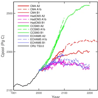
Fig. 1.Evolution of the global terrestrial ecosystem carbon pool (Cpool) under twelve future scenario simulations with LPJ-GUESS.

To attribute variation in the resultant carbon balance time series to underlying forcing factors, we performed analysis of variance (ANOVA; Draper and Smith 1998) with α, γ, and [CO2] pathway (A2, A1B, B1) as independent factors.

The ANOVA gives information on which factor induces the largest spread in simulated total carbon pool by the statis-tical emulator. It separates the total sum of squares in the simulated change in total carbon stock from 2000–2099 into sum of squares due to each of the three factors above and a residual term that contains effects due to interactions be-tween factors and an unexplained component, such as tem-perature. Since the temperature depends on the specific CO2

scenario, it is non-trivial to quantify the effect of different temperatures, forcing us to limit the ANOVA to the three fac-torsα,γ, and CO2.

3 Results

3.1 Carbon cycle simulations

The LPJ-GUESS simulations forced by different GCMs and [CO2] pathways result in a wide range of trajectories for

Cpool (Fig. 1). Simulations forced by climate data from the same GCM under different CO2emission scenarios tend to

cluster, indicating that differences between GCMs exert a stronger control on Cpool than [CO2] pathways. By 2099,

(6)

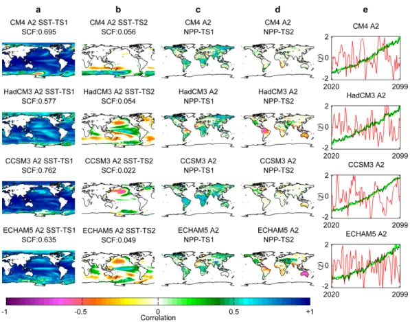
Fig. 2.Spatial patterns of correlation (Pearsonr) between the first two EOF modes of GCM-simulated SST under the A2 scenario and the original simulated SST and simulated NPP.(a)Correlations between original SST and the time series of the first EOF mode (TS1; green line in(e)).(b)Correlations between original SST and the time series of the second EOF mode (TS2; red line in(e)).(c)Correlations between simulated NPP and the time series of the first EOF mode.(d)Correlations between simulated NPP and the time series of the second EOF mode.(e)Standardized time series (Z-scores) with mean zero and standard deviation one, of the first EOF mode, TS1, (green), second EOF mode, TS2, (red) and global land temperature (black). The correlations presented in colours are all statistically significant at 5 % level.

3.2 GCM climate–carbon cycle relationships

The EOF time series of the first two modes, the SST spa-tial correlation patterns and the NPP correlation patterns for the time period 2020–2099 are illustrated in Fig. 2. The first mode is closely related to the global temperature trend and variability as indicated by the overall strong correlation over all the world’s oceans (Fig. 2a). The temporal variability and trend of the first mode show similarities with the standard-ized global land temperatures (Fig. 2e). The SCF differs be-tween the GCMs. A high SCF in the first mode implies a rel-atively uniform pattern of SST variability across the globe, as seen for CCSM3, while a lower SCF in the first mode, as seen for HadCM3 and ECHAM5, implies that differences in SST variability in different areas of the world’s oceans more strongly contribute to the total variability globally.

The second mode of variability (Fig. 2b) explains around an order of magnitude less of the total variance of the simu-lated SSTs for all four GCMs, and is generally characterized by El Ni˜no-Southern Oscillation (ENSO) like patterns,

domi-nated by variability in the central tropical Pacific. The ENSO patterns are more prominent in the SSTs of ECHAM5 and HadCM3 compared with the other GCMs, while for CM4 they are more pronounced in the third mode (not shown here) than in the second mode, indicating that other variation, not primarily associated with ENSO, is influencing the second mode of variability for this GCM. Time series for the first two modes (Fig. 2e) show, as expected, a uniform up-going trend in the first mode consistent with global warming response to rising greenhouse gas concentrations, while the second mode exhibits continuous fluctuations with no obvious trends for any of the models.

The third and fourth columns (Fig. 2c–d) show the cor-relation between the modes and simulated NPP. Global tem-perature increase, together with the covarying [CO2] (closely

(7)

1901 2000 2100 2100

2300 2500

C M4 A2

1901 2000 2100 2200 C M4 A1b

1901 2000 2100 2200 C M4 B 1

1901 2000 2100

2100 2300 2500

HadC M3 A2

1901 2000 2100 2200 HadC M3 A1b

1901 2000 2100 2200 HadC M3 B 1

1901 2000 2100

2100 2300 2500

C C S M3 A2

1901 2000 2100 2200 C C S M3 A1b

1901 2000 2100 2200 C C S M3 B 1

1901 2000 2100

2100 2300 2500

E C HAM5 A2

1901 2000 2100 2200 E C HAM5 A1b

1901 2000 2100 2200 E C HAM5 B 1

Y ear

C

p

o

l

(P

g

C

)

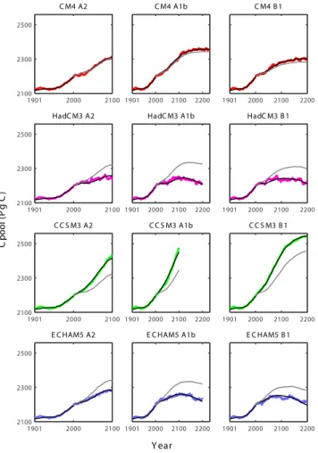
Fig. 3.Global terrestrial ecosystem carbon pool (Cpool) as simu-lated by LPJ-GUESS (colours) and the dynamic replacement model with averageα(grey) or simulation-specific fit forα(black).

America and western North Africa see a decreased NPP re-sulting from the negative impacts of decreased precipitation and/or increased evapotranspiration under higher tempera-tures on plant water relations (Supplement Fig. S3).

The correlation patterns between the second mode and NPP (Fig. 2d) illustrate the impact of ENSO-related regional climate patterns on land ecosystems, particularly water re-lations. For HadCM3, ENSO leads to pronounced decrease of NPP in the tropics and Australia and increased NPP in western North America and the Middle East. In ECHAM5 the negative impact is more pronounced in Australia but less pronounced in the tropics. The regions that show increased NPP are similar for both GCMs. The direct cause of the NPP declines in HadCM3 and ECHAM5 is decreased precipita-tion and increased temperature (Supplement Fig. S3).

CCSM3 shows a similar but considerably weaker corre-lation pattern compared to ECHAM5, while CM4 shows no strong patterns, probably because ENSO dynamics for that GCM are expressed mainly in the third mode. Correlation patterns between SST modes and NBP, shown in Fig. S4, are generally reminiscent of the results for NPP, reflecting the

0.3 0.4

−11 −10 −9 −8 −7 −6 −5 −4 −3 −2

CM4 A2 CM4 A1b CM4 B1 HadCM3 A2 HadCM3 A1b HadCM3 B1 CCSM3 A2 CCSM3 A1b ECHAM5 A2 ECHAM5 A1b ECHAM5 B1

SST Standard Deviation °C

α

(Pg C/y)

Fig. 4.Relation between the simulation-specific parameterαand global SST variability.

driving role of vegetation productivity in the carbon cycling of ecosystems as a whole.

3.3 GCM-dependent uncertainty in carbon balance

GCM-simulated global mean land temperature and the [CO2]

pathway of the underlying emission scenario explain part, but not all, of the variation between simulations in the evo-lution of the terrestrial carbon pool over the 21st century, as simulated by LPJ-GUESS. The remaining, unexplained, source of variation, signified by αin Eq. (2), encapsulates the regional patterns of carbon balance and their evolu-tion over time, specific to each GCM×emissions scenario combination (Fig. 3). The displacement between the black (simulation-specific fit forα)and grey (αset to the average of the twelve simulation-specific values) curve in each frame of Fig. 3 represents the effect of this unexplained variation in each individual simulation.

The EOF analysis reveals differences in the impact on sim-ulated NPP and NBP, induced by differences among GCMs related to SST variability and associated weather patterns (see Fig. 2). We found a strong relationship betweenαand global SST variability (Fig. 4). Theαvalues cluster accord-ing to GCMs and not accordaccord-ing to CO2 emission

(8)

negativeαvalues of all the simulations. All simulations have anα value lower than the historical simulation (for which

α=0).

3.4 Global versus land temperature

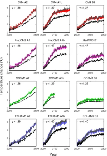
The ratio of land to global warmingγ varied from 1.26 to 1.46 between the 12 datasets for 2001–2009 (Fig. 5). CCSM3 shows the lowest γ (least amplification of warming over land) among all scenarios while HadCM3 shows the largest

γ among all scenarios. A single GCM-specific factor seems to be enough to explain most variation inγas long as the cli-mate forcing is increasing. In the longest dataset used here, the CM4 A1B, top, middle column in Fig. 5, where [CO2]

has been held constant since 2100, land temperatures have started to diverge from the constant warming amplification seen during the 21st century, approaching the global tem-peratures. The range in A2 global temperature (2095–2099) is 0.27◦

C, while the range in land temperatures is more than double this at 0.57◦

C. The global average temperature change,1GT, (2095–2099) in the HadCM3 model’s A2 sce-nario is the lowest among the four GCMs (3.9◦

C), while the land temperature,1LT, for the same period, GCM and sce-nario is the highest among the GCMs (5.7◦

C).

3.5 Partitioning uncertainty in carbon balance

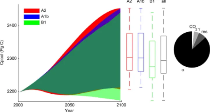
Using the statistical carbon balance emulator to sample across 192 combinations of GCM and scenario characteris-tics (see Methods), we came up with the distribution of car-bon balance trajectories shown in Fig. 6. For this ensemble of [CO2] pathways and GCMs, and given the carbon cycle

representation in LPJ-GUESS, total terrestrial carbon stocks may increase or decrease by the end of the 21st century, but are more likely to increase. Note that the percentiles and the medians shown in Fig. 6 are partly a result of the sampling. It is apparent that much of the uncertainty represented by the spread among trajectories propagates from different charac-teristics and behaviour of GCMs. According to the ANOVA analysis, 91 % of the variability among trajectories could be explained by the two GCM-specific factorsα(87 %) andγ

(5 %). The choice of CO2emission scenario explains just 2 %

of the variation, while 7 % remains unexplained (Fig. 6).

4 Discussion

The LPJ-GUESS simulations forced by the ensemble of GCMs and CO2emission scenarios chosen for this study

re-sult in a considerable spread in the future evolution of car-bon balance. Our results demonstrate that the majority of this spread can be traced to a GCM-specific parameter (α)closely related to global SST variability.

As seen in Fig. 4, all the GCMs show a negativeαvalue (αwas set to 0 for CRU). One interpretation could be that all GCMs show increasing climate variability or other

cli-20000 2100

2 4 6

CM4 A2

γ =1.38

2000 2100 2200

CM4 A1b

γ =1.39

2000 2100 2200

CM4 B1

γ =1.37

20000 2100

2 4 6

HadCM3 A2

γ =1.46

2000 2100 2200

HadCM3 A1b

γ =1.47

2000 2100 2200

HadCM3 B1

γ =1.47

20000 2100

2 4 6

CCSM3 A2

γ =1.28

2000 2100 2200

CCSM3 A1b

γ =1.29

2000 2100 2200

CCSM3 B1

γ =1.26

20000 2100

2 4 6

ECHAM5 A2

γ =1.39

2000 2100 2200

ECHAM5 A1b

γ =1.40

2000 2100 2200

ECHAM5 B1

γ =1.40

Year

Temperature change (

°

C)

Fig. 5.Average global temperature change,1GT (black), average global land temperature change1LT (colours) and average global land temperature estimated byγ×1GT (grey).

mate characteristics that negatively influence GPP. However, the offset of the α values in comparison to CRU can also be explained by the offset between the GCMs and CRU as a result of different trends since the 1961–1990 climatology. Additionally, as a result of station data limitations, around 13 % of the CRU gridcells used in this study show at least one consecutive 10-yr period with no interannual variability (see Supplement Fig. S5). Although the importance of these episodes in the CRU data for the simulated carbon balance is unknown, it is difficult to draw conclusions about theα

values.

(9)

Fig. 6.Results of the 192 replacement model simulations using “ar-tificial GCM” input. The total spread of the A2 scenario simula-tions in total terrestrial carbon pool (Cpool) is illustrated in red. Blue shows the A1B scenario and green the B1 scenario. The box-plots show the median, 25th and 75th percentile, and maximum and minimum values of the 2099 total terrestrial carbon pool (Pg C), for each CO2scenario and all simulations. The pie chart shows the

proportion of 2099 total carbon pool variability explained by,α,γ, CO2scenarios and residual unexplained variation (res.).

also considered. Different land use projections, as well as dif-ferent treatment of land use and land use change in DGVMs and carbon cycle models, constitute a large source of uncer-tainty as to future carbon balance (e.g. Zaehle et al., 2007). Still, our results provide some quantification of GCM dis-crepancies and their impact on carbon balance as simulated by our model.

By applying different GCMs and scenarios to force a sin-gle ecosystem model, LPJ-GUESS, we have focused on the uncertainties arising from differences in the climate as pro-jected by the GCMs. Previous studies show that different DGVMs can project substantially different carbon balance in response to the same forcing (Cramer et al., 2001; Sitch et al., 2008; Piao et al., 2013). This carbon cycle model-dependent aspect of the overall uncertainty has not been addressed in this study. However, LPJ-GUESS shows comparable skill and behaviour to other DGVMs and may be regarded as rep-resentative of DGVMs as a group in terms global carbon bal-ance response to climate and [CO2] forcing. For example,

a recent study comparing ten DGVMs with each other and with independent datasets (Piao et al., 2013) shows that LPJ-GUESS predicts present day global GPP in the middle of the range of other models, in agreement with an observation-based estimate, and exhibits comparable sensitivity to pre-cipitation as suggested by upscaled ecosystem flux measure-ments.

When applying the statistical emulator with combinations of the GCM-specific parameters and variables we assume that they are independent. When averagingγ andαacross GCMs (n=4), they show no significant correlation (r= −₀.93, n.s.) but when we use all simulations (n=_{12), they} show a significant correlation (r= −₀.92, P <0.00005). However, this high correlation could be a coincidence

result-ing from the specific selection of GCMs. Amongst many fac-tors and processes it is plausible that GCM differences, for example in the partitioning of latent and sensible heat fluxes between the surface and atmosphere can influence both α

andγ. Other possible differences between GCMs, such as differences in ocean overturning or the melting of sea ice af-fecting ocean warming, potentially influencingγ are likely to have smaller effect on α. ENSO is the dominant deter-minant of global precipitation variability (Dai et al., 1997). A prominent effect of warm ENSO events is negative pre-cipitation anomalies in large parts of the tropics, but also significant precipitation anomalies in other regions can be traced back to ENSO (Dai and Wigley, 2000). Patterns of correlation between pacific SST variability and precipitation reminiscent of ENSO have been found to emerge in GCM simulations. The EOF analysis of sea surface temperatures presented here reveals carbon cycle patterns similar to those found by Dai (2006) when analysing rainfall patterns and tropical SST variability in HadCM3, ECHAM5 and CCSM3, amongst other GCMs. Although the “strength” of representa-tion of ENSO differs between GCMs, a strong dependency of low latitude precipitation and tropical SST variability is typ-ically simulated on interannual and longer timescales (Dai, 2006).

(10)

5 Conclusions

Our results point to a marked dependency of the future de-velopment of global terrestrial ecosystem carbon balance on climate characteristics, particularly SST variability and its impact on weather patterns, simulated differently among dif-ferent GCMs. A further GCM characteristic, the degree of enhancement of warming over land relative to global warm-ing generally, accounts for the second largest proportion of uncertainty in carbon balance response. Uncertainty stem-ming from the choice of CO2emission scenario is much less

marked. Finally, our results suggest that improved represen-tations of ENSO dynamics and low-latitude precipitation pat-terns are important to narrow the uncertainties in future cli-mate change projections using ESMs or uncoupled DGVMs forced by GCM-simulated climate projections.

Supplementary material related to this article is available online at: http://www.biogeosciences.net/10/ 1517/2013/bg-10-1517-2013-supplement.pdf.

Acknowledgements. This study was funded by the Foundation for Strategic Environment Research (Mistra) through the Mistra-SWECIA programme. The study is a contribution to the Lund University Strategic Research Areas Modelling the Regional and Global Earth System (MERGE) and Biodiversity and Ecosystem Services in a Changing Climate (BECC). We acknowledge the global modelling groups, the Program for Climate Model Diagnosis and Intercomparison (PCMDI) and the WCRP’s Working Group on Coupled Modelling (WGCM) for their roles in making available the WCRP CMIP3 multimodel dataset. Support of this dataset is provided by the Office of Science, US Department of Energy.

Edited by: M. Dai

References

Ahlstr¨om, A., Miller, P. A., and Smith, B.: Too early to infer a global NPP decline since 2000, Geophys. Res. Lett., 39, L15403, doi:10.1029/2012gl052336, 2012a.

Ahlstr¨om, A., Schurgers, G., Arneth, A., and Smith, B.: Robust-ness and uncertainty in terrestrial ecosystem carbon response to CMIP5 climate change projections, Environ. Res. Lett., 7, 044008, doi:10.1088/1748-9326/7/4/044008, 2012b.

Berthelot, M., Friedlingstein, P., Ciais, P., Dufresne, J.-L., and Mon-fray, P.: How uncertainties in future climate change predictions translate into future terrestrial carbon fluxes, Glob. Change Biol., 11, 959–970, doi:10.1111/j.1365-2486.2005.00957.x, 2005. Brando, P. M., Nepstad, D. C., Davidson, E. A., Trumbore, S. E.,

Ray, D., and Camargo, P.: Drought effects on litterfall, wood production and belowground carbon cycling in an Amazon for-est: results of a throughfall reduction experiment, Philosophical Transactions of the Royal Society B, Biol. Sci., 363, 1839–1848, doi:10.1098/rstb.2007.0031, 2008.

Canadell, J. G., Le Qu´er´e, C., Raupach, M. R., Field, C. B., Buiten-huis, E. T., Ciais, P., Conway, T. J., Gillett, N. P., Houghton, R. A., and Marland, G.: Contributions to accelerating atmospheric CO2 growth from economic activity, carbon intensity, and effi-ciency of natural sinks, Proc. Natl. Ac. Sci., 104, 18866–18870, doi:10.1073/pnas.0702737104, 2007.

Collins, W. D., Bitz, C. M., Blackmon, M. L., Bonan, G. B., Bretherton, C. S., Carton, J. A., Chang, P., Doney, S. C., Hack, J. J., Henderson, T. B., Kiehl, J. T., Large, W. G., McKenna, D. S., Santer, B. D., and Smith, R. D.: The Community Climate System Model Version 3 (CCSM3), J. Clim., 19, 2122–2143, doi:10.1175/jcli3761.1, 2006.

Cramer, W., Bondeau, A., Woodward, F. I., Prentice, I. C., Betts, R. A., Brovkin, V., Cox, P. M., Fisher, V., Foley, J. A., Friend, A. D., Kucharik, C., Lomas, M. R., Ramankutty, N., Sitch, S., Smith, B., White, A., and Young-Molling, C.: Global re-sponse of terrestrial ecosystem structure and function to CO2 and climate change: results from six dynamic global vegetation models, Glob. Change Biol., 7, 357–373, doi:10.1046/j.1365-2486.2001.00383.x, 2001.

Dai, A.: Precipitation Characteristics in Eighteen Coupled Climate Models, J. Clim., 19, 4605–4630, doi:10.1175/jcli3884.1, 2006. Dai, A.: Increasing drought under global warming in

ob-servations and models, Nature Clim. Change, 3, 52–58, doi:10.1038/nclimate1633, 2013.

Dai, A. and Wigley, T. M. L.: Global Patterns of ENSO-induced Precipitation, Geophys. Res. Lett., 27, 1283–1286, doi:10.1029/1999gl011140, 2000.

Dai, A., Fung, I. Y., and Del Genio, A. D.: Surface Ob-served Global Land Precipitation Variations during 1900–1988, J. Clim., 10, 2943–2962, doi:10.1175/1520-0442(1997)010¡2943:soglpv¿2.0.co;2, 1997.

Denman, K. L.,Brasseur, G. , Chidthaisong, A., Ciais, P., Cox, P. M., Dickinson, R. E., Hauglustaine, D., Heinze, C., Holland, E., Jacob, D., Lohmann, U., Ramachandran, S., da Silva Dias, P. L., Wofsy, S. C., and Zhang, X.: Couplings Between Changes in the Climate System and Biogeochemistry, in: Climate Change 2007: The Physical Science Basis, Contribution of Working Group I to the Fourth Assessment Report of the Intergovernmental Panel on Climate Change, edited by: Solomon, S., Qin, D., Manning, M., Chen, Z., Marquis, M., Averyt, K. B., Tignor, M. , and Miller, H. L., Cambridge University Press, Cambridge, United Kingdom and New York, NY, USA, 499–587, 2007.

Draper, N. and Smith, H.: Applied regression analysis, Wiley Series in Probability and Statistics, Wiley-Interscience, New York, 736 pp., 1998.

Friedlingstein, P., Cox, P., Betts, R., Bopp, L., von Bloh, W., Brovkin, V., Cadule, P., Doney, S., Eby, M., Fung, I., Bala, G., John, J., Jones, C., Joos, F., Kato, T., Kawamiya, M., Knorr, W., Lindsay, K., Matthews, H. D., Raddatz, T., Rayner, P., Re-ick, C., Roeckner, E., Schnitzler, K.-G., Schnur, R., Strassmann, K., Weaver, A. J., Yoshikawa, C., and Zeng, N.: Climate–Carbon Cycle Feedback Analysis: Results from the C4MIP Model Inter-comparison, J. Clim., 19, 3337–3353, doi:10.1175/JCLI3800.1, 2006.

(11)

Gordon, C., Cooper, C., Senior, C. A., Banks, H., Gregory, J. M., Johns, T. C., Mitchell, J. F. B., and Wood, R. A.: The simulation of SST, sea ice extents and ocean heat transports in a version of the Hadley Centre coupled model without flux adjustments, Clim. Dyn., 16, 147–168, doi:10.1007/s003820050010, 2000. Hickler, T., Prentice, I. C., Smith, B., Sykes, M. T., and Zaehle, S.:

Implementing plant hydraulic architecture within the LPJ Dy-namic Global Vegetation Model, Glob. Ecol. Biogeogr., 15, 567– 577, doi:10.1111/j.1466-8238.2006.00254.x, 2006.

Hickler, T., Vohland, K., Feehan, J., Miller, P. A., Smith, B., Costa, L., Giesecke, T., Fronzek, S., Carter, T. R., Cramer, W., K¨uhn, I., and Sykes, M. T.: Projecting the future distribution of Euro-pean potential natural vegetation zones with a generalized, tree species-based dynamic vegetation model, Glob. Ecol. Biogeogr., 21, 50–63, doi:10.1111/j.1466-8238.2010.00613.x, 2012. Hoerling, M., Eischeid, J., and Perlwitz, J.: Regional Precipitation

Trends: Distinguishing Natural Variability from Anthropogenic Forcing, J. Clim., 23, 2131–2145, doi:10.1175/2009jcli3420.1, 2009.

Huete, A. R., Didan, K., Shimabukuro, Y. E., Ratana, P., Saleska, S. R., Hutyra, L. R., Yang, W., Nemani, R. R., and Myneni, R.: Amazon rainforests green-up with sunlight in dry season, Geo-phys. Res. Lett., 33, L06405, doi:10.1029/2005gl025583, 2006. Knutti, R. and Hegerl, G. C.: The equilibrium sensitivity of the

Earth’s temperature to radiation changes, Nature Geosci., 1, 735– 743, 2008.

Le Qu´er´e, C., Raupach, M. R., Canadell, J. G., Marland, G., Bopp, L., Ciais, P., and Conway, T. J.: Trends in the sources and sinks of carbon dioxide, Nature Geosci., 2, 831–836, doi:10.1038/ngeo689, 2009.

Malhi, Y., Roberts, J. T., Betts, R. A., Killeen, T. J., Li, W., and Nobre, C. A.: Climate Change, Deforestation, and the Fate of the Amazon, Science, 319, 169–172, doi:10.1126/science.1146961, 2008.

Marti, O., Braconnot, P., Bellier, J., Benshila, R., Bony, S., Brock-mann, P., Cadule, P., Caubel, A., Denvil, S., Dufresne, J. L., Fair-head, L., Filiberti, M.-A., Fichefet, T., Foujols, M.-A., Friedling-stein, P., Grandpeix, J.-Y., Hourdin, F., Krinner, G., L´evy, C., Madec, G., Musat, I., De Noblet, N., Polcher, J., and Talandier, C.: The new IPSL climate system model: IPSL-CM4, 1–86, 2005.

Meehl, G. A., Covey, C., Delworth, T., Latif, M., McAvaney, B., Mitchell, J. F. B., Stouffer, R. J., and Taylor, K. E.: The WCRP CMIP3 Multimodel Dataset: A New Era in Climate Change Re-search, Bull. Am. Meteorol. Soc., 88, 1383–1394, 2007a. Meehl, G. A., Stocker, T., Collins, W., Friedlingstein, A., Gaye,

A., Gregory, J., Kitoh, A., Knutti, R., Murphy, J., and Noda, A.: Global climate projections, in: Climate Change 2007: The Physi-cal Science Basis. Contribution of Working Group 1 to the Fourth Assessment report of the Intergovernmental Panel on Climate Change, edited by: Solomon, S., Qin, D., Manning, M., Chen, Z., Marquis, M., Averyt, K., Tignor, M., and Miller, H., Cam-bridge University Press, CamCam-bridge, United kingdom and New York, NY, USA, 747–845, 2007b.

Mitchell, T. D. and Jones, P. D.: An improved method of con-structing a database of monthly climate observations and as-sociated high-resolution grids, Int. J. Climatol., 25, 693–712, doi:10.1002/joc.1181, 2005.

Morales, P., Sykes, M. T., Prentice, I. C., Smith, P., Smith, B., Bugmann, H., Zierl, B., Friedlingstein, P., Viovy, N., Sabat´e, S., S´anchez, A., Pla, E., Gracia, C. A., Sitch, S., Arneth, A., and Ogee, J.: Comparing and evaluating process-based ecosys-tem model predictions of carbon and water fluxes in major European forest biomes, Glob. Change Biol., 11, 2211–2233, doi:10.1111/j.1365-2486.2005.01036.x, 2005.

Morales, P., Hickler, T., Rowell, D. P., Smith, B., and Sykes, M. T.: Changes in European ecosystem productivity and carbon balance driven by regional climate model output, Glob. Change Biol., 13, 108–122, doi:10.1111/j.1365-2486.2006.01289.x, 2007. Nakicenovic, N., Alcamo, J., Davis, G., de Vries, B., Fenhann, J.,

Gaffin, S., Gregory, K., Grubler, A., Jung, T. Y., Kram, T., La Rovere, E. L., Michaelis, L., Mori, S., Morita, T., Pepper, W., Pitcher, H. M., Price, L., Riahi, K., Roehrl, A., Rogner, H.-H., Sankovski, A., Schlesinger, M., Shukla, P., Smith, S. J., Swart, R., van Rooijen, S., Victor, N., and Dadi, Z.: IPCC Special Re-port on Emissions Scenarios: a special reRe-port of Working Group III of the Intergovernmental Panel on Climate Change, edited by: Nakicenovic, N. and Swart, R., Cambridge University Press, Cambridge, UK, 2000.

Nepstad, D. C., Tohver, I. M., Ray, D., Moutinho, P., and Cardinot, G.: Mortality of Large Trees and Lianas Following Experimen-tal Drought in an Amazon Forest, Ecology, 88, 2259–2269, doi:10.1890/06-1046.1, 2007.

Phillips, O. L., Aragão, L. E. O. C., Lewis, S. L., Fisher, J. B., Lloyd, J., López-González, G., Malhi, Y., Monteagudo, A., Pea-cock, J., Quesada, C. A., van der Heijden, G., Almeida, S., Amaral, I., Arroyo, L., Aymard, G., Baker, T. R., Bánki, O., Blanc, L., Bonal, D., Brando, P., Chave, J., de Oliveira, Á. C. A., Cardozo, N. D., Czimczik, C. I., Feldpausch, T. R., Freitas, M. A., Gloor, E., Higuchi, N., Jiménez, E., Lloyd, G., Meir, P., Mendoza, C., Morel, A., Neill, D. A., Nepstad, D., Patiño, S., Peñuela, M. C., Prieto, A., Ram´ırez, F., Schwarz, M., Silva, J., Silveira, M., Thomas, A. S., Steege, H. T., Stropp, J., Vásquez, R., Zelazowski, P., Dávila, E. A., Andelman, S., Andrade, A., Chao, K.-J., Erwin, T., Di Fiore, A., Eur´ıdice, H. C., Keeling, H., Killeen, T. J., Laurance, W. F., Cruz, A. P., Pitman, N. C. A., Vargas, P. N., Ram´ırez-Angulo, H., Rudas, A., Salamão, R., Silva, N., Terborgh, J., and Torres-Lezama, A.: Drought Sen-sitivity of the Amazon Rainforest, Science, 323, 1344–1347, doi:10.1126/science.1164033, 2009.

Piao, S., Sitch, S., Ciais, P., Friedlingstein, P., Peylin, P., Wang, X., Ahlstr¨om, A., Alessandro, A., Canadell, J. G., Huntingford, C., Jung, M., Levis, S., Levy, P. E., Lomas, M. R., Luo, Y., Myneni, R. B., Poulter, B., Viovy, N., Zaehle, S., and Zeng, N.: Evalua-tion of terrestrial carbon cycle models for their sensitivity to cli-mate changes and rising atmospheric CO2concentrations, Glob.

Change Biol., accepted, 2013.

Quadrelli, R. and Wallace, J. M.: A Simplified Linear Framework for Interpreting Patterns of Northern Hemisphere Wintertime Climate Variability, J. Clim., 17, 3728–3744, doi:10.1175/1520-0442(2004)017¡3728:aslffi¿2.0.co;2, 2004.

(12)

Saleska, S. R., Didan, K., Huete, A. R., and da Rocha, H. R.: Ama-zon Forests Green-Up During 2005 Drought, Science, 318, p. 612, doi:10.1126/science.1146663, 2007.

Schaphoff, S., Lucht, W., Gerten, D., Sitch, S., Cramer, W., and Prentice, I.: Terrestrial biosphere carbon storage under alternative climate projections, Clim. Change, 74, 97–122, doi:10.1007/s10584-005-9002-5, 2006.

Sitch, S., Smith, B., Prentice, I. C., Arneth, A., Bondeau, A., Cramer, W., Kaplan, J. O., Levis, S., Lucht, W., Sykes, M. T., Thonicke, K., and Venevsky, S.: Evaluation of ecosystem dynam-ics, plant geography and terrestrial carbon cycling in the LPJ dy-namic global vegetation model, Glob. Change Biol., 9, 161–185, doi:10.1046/j.1365-2486.2003.00569.x, 2003.

Sitch, S., Huntingford, C., Gedney, N., Levy, P. E., Lomas, M., Piao, S. L., Betts, R., Ciais, P., Cox, P., Friedlingstein, P., Jones, C. D., Prentice, I. C., and Woodward, F. I.: Evalua-tion of the terrestrial carbon cycle, future plant geography and climate-carbon cycle feedbacks using five Dynamic Global Veg-etation Models (DGVMs), Glob. Change Biol., 14, 2015–2039, doi:10.1111/j.1365-2486.2008.01626.x, 2008.

Smith, B., Prentice, I. C., and Sykes, M. T.: Representation of vegetation dynamics in the modelling of terrestrial ecosystems: comparing two contrasting approaches within European climate space, Glob. Ecol. Biogeogr., 10, 621–637, doi:10.1046/j.1466-822X.2001.t01-1-00256.x, 2001.

Smith, B., Knorr, W., Widlowski, J.-L., Pinty, B., and Gobron, N.: Combining remote sensing data with process modelling to mon-itor boreal conifer forest carbon balances, Forest Ecol. Manage., 255, 3985–3994, doi:10.1016/j.foreco.2008.03.056, 2008. Smith, B., Samuelsson, P., Wramneby, A., and Rummukainen, M.:

A model of the coupled dynamics of climate, vegetation and terrestrial ecosystem biogeochemistry for regional applications, Tellus A, 63, 87–106, doi:10.1111/j.1600-0870.2010.00477.x, 2011.

Tang, G., Beckage, B., Smith, B., and Miller, P. A.: Estimating po-tential forest NPP, biomass and their climatic sensitivity in New England using a dynamic ecosystem model, Ecosphere, 1, 18 pp., doi:10.1890/es10-00087.1, 2010.

Tang, G., Beckage, B., and Smith, B.: The potential transient dy-namics of forests in New England under historical and projected future climate change, Clim. Change, 1–21, doi:10.1007/s10584-012-0404-x, 2012.

Toomey, M., Roberts, D. A., Still, C., Goulden, M. L., and McFad-den, J. P.: Remotely sensed heat anomalies linked with Amazo-nian forest biomass declines, Geophys. Res. Lett., 38, L19704, doi:10.1029/2011gl049041, 2011.

Uvo, C. and Berndtsson, R.: Regionalization and spatial properties of Cear´a State rainfall in northeast Brazil, J. Geophys. Res. At-mos., 101, 4221–4233, doi:10.1029/95jd03235, 1996.

Uvo, C. B., Repelli, C. A., Zebiak, S. E., and Kushnir, Y.: The Relationships between Tropical Pacific and Atlantic SST and Northeast Brazil Monthly Precipitation, J. Clim., 11, 551–562, doi:10.1175/1520-0442(1998)011¡0551:trbtpa¿2.0.co;2, 1998. Wallace, J. M., Zhang, Y., and Lau, K.-H.: Structure and

Season-ality of Interannual and Interdecadal Variability of the Geopo-tential Height and Temperature Fields in the Northern Hemi-sphere TropoHemi-sphere, J. Clim., 6, 2063–2082, doi:10.1175/1520-0442(1993)006¡2063:sasoia¿2.0.co;2, 1993.

Wilks, D. S.: Statistical Methods in the Atmospheric Sciences, 2nd Edn., Academic Press, Burlington, MA, USA, San Diego, CA, USA, London, UK, 627 pp., 2006.

Wramneby, A., Smith, B., Zaehle, S., and Sykes, M. T.: Parame-ter uncertainties in the modelling of vegetation dynamics – Ef-fects on tree community structure and ecosystem functioning in European forest biomes, Ecological Modelling, 216, 277-290, 10.1016/j.ecolmodel.2008.04.013, 2008.

Zaehle, S., Sitch, S., Prentice, I. C., Liski, J., Cramer, W., Erhard, M., Hickler, T., and Smith, B.: The Importance of Age-Related Decline in Forest NPP for Modeling Regional Carbon Balances, Ecol. Appl., 16, 1555–1574, 2006.

Zaehle, S., Bondeau, A., Carter, T., Cramer, W., Erhard, M., Pren-tice, I. C., Reginster, I., Rounsevell, M. A., Sitch, S., Smith, B., Smith, P., and Sykes, M.: Projected Changes in Terrestrial Carbon Storage in Europe under Climate and Land-use Change, 1990–2100, Ecosystems, 10, 380–401, doi:10.1007/s10021-007-9028-9, 2007.