A global climatology of stratospheric OClO derived from GOMOS measurement

(1)

AMTD

6, 3511–3543, 2013

A global climatology of stratospheric OClO

C. T ´etard et al.

Title Page

Abstract Introduction

Conclusions References

Tables Figures

◭ ◮

Back Close

Full Screen / Esc

Printer-friendly Version Interactive Discussion

Discussion

P

a

per

|

Dis

cussion

P

a

per

|

Discussion

P

a

per

|

Discussio

n

P

a

per

|

Atmos. Meas. Tech. Discuss., 6, 3511–3543, 2013 www.atmos-meas-tech-discuss.net/6/3511/2013/ doi:10.5194/amtd-6-3511-2013

Atmospheric Measurement

Techniques

Open Access

Discussions

Geoscientiic Geoscientiic

This discussion paper is/has been under review for the journal Atmospheric Measurement Techniques (AMT). Please refer to the corresponding final paper in AMT if available.

A global climatology of stratospheric

OClO derived from GOMOS measurement

C. T ´etard1, D. Fussen1, F. Vanhellemont1, C. Bingen1, E. Dekemper1,

N. Mateshvili1, D. Pieroux1, C. Robert1, E. Kyr ¨ol ¨a2, J. Tamminen2, V. Sofieva2,

A. Hauchecorne3, F. Dalaudier3, J.-L. Bertaux3, O. Fanton d’Andon4, G. Barrot4,

L. Blanot4, A. Dehn5, and L. Saavedra de Miguel6

1

Institut d’A ´eronomie Spatiale de Belgique, Brussels, Belgium 2

Finnish Meteorological Institute, Earth Observation, Helsinki, Finland 3

Laboratoire Atmosph `eres, Milieux, Observations Spatiales, CNRS-INSU, Univ. Versailles St-Quentin, Guyancourt, France

4

ACRI-ST, Sophia-Antipolis, France 5

European Space Research Institute (ESRIN), European Space Agency, Frascati, Italy 6

IDEAS, Serco, Frascati, Italy

Received: 27 February 2013 – Accepted: 3 April 2013 – Published: 11 April 2013

Correspondence to: C. T ´etard ([email protected])

(2)

AMTD

6, 3511–3543, 2013

C. T ´etard et al.

Title Page

Tables Figures

◭ ◮

Back Close

Full Screen / Esc

Discussion

P

a

per

|

Dis

cussion

P

a

per

|

Discussion

P

a

per

|

Discussio

n

P

a

per

|

Abstract

The Global Ozone Monitoring by Occultation of Stars (GOMOS) instrument on board the European platform ENVISAT was dedicated to the study of the atmosphere of the Earth using the stellar occultation technique. The spectral range of the GOMOS spec-trometer extends from the UV to the near infrared, allowing for the retrieval of species

5

such as O3, NO2, NO3, H2O, O2, air density, aerosol extinction and OClO.

Never-theless, OClO can not be retrieved using a single GOMOS measurement because of the weak signal-to-noise ratio and the small optical thickness associated with this molecule. We present here the method used to detect this molecule by using several GOMOS measurements. It is based on a two-step approach. First, several co-located

10

measurements are combined in a statistical way to build an averaged measurement with a higher signal-to-noise ratio. Then, a Differential Optical Absorption Spectroscopy (DOAS) method is applied to retrieve OClO slant column densities. The statistics of the sets of GOMOS measurements used to build the averaged measurement and the spec-tral window selection are analyzed. The obtained retrievals are compared to results

15

from two balloon-borne instruments. It appears that the inter-comparisons of OClO are generally satisfying. Then, two nighttime climatologies of OClO slant column densities based on GOMOS averaged measurements are presented. The first depicts annual global pictures of OClO from 2003 to 2011. From this climatology, the presence of an OClO layer in the equatorial region at about 35 km is confirmed and strong

concen-20

trations of OClO in both polar regions are observed, a sign of chlorine activation. The second climatology is a monthly time series. It clearly shows the chlorine activation of the lower stratosphere during winter. Moreover the equatorial OClO layer is observed during all the years without any significant variations. Finally, the anti-correlation be-tween OClO and NO2is highlighted. This very promising method, applied on GOMOS

25

(3)

AMTD

6, 3511–3543, 2013

C. T ´etard et al.

Title Page

Tables Figures

◭ ◮

Back Close

Full Screen / Esc

Discussion

P

a

per

|

Dis

cussion

P

a

per

|

Discussion

P

a

per

|

Discussio

n

P

a

per

|

1 Introduction

The discovery of the stratospheric ozone depletion in Antarctica by Farman et al. (1985) has led to numerous studies to understand the physico-chemical mechanisms involved in this recurrent phenomenon. It appears that the halogen species play an important role in the chemical cycles that lead to polar ozone depletion (Solomon et al., 1986).

5

Of these cycles, those involving active chlorine species (Cl, ClO, Cl2O2) are among

the most e_fficient (Salawitch et al., 1993). The presence of chlorine species in the atmosphere is mainly due to the emission of chlorofluorocarbons (CFC) at the ground. CFCs are chemically inert in the troposphere and are not soluble in water, which make them resistant to washout processes. Therefore, they are efficiently transported toward

10

the stratosphere where they are photolyzed by UV radiation or oxidized to produce atomic chlorine and chlorine monoxide (ClO). One consequence of the accumulation of ClO in the stratosphere is the formation of chlorine dioxide (OClO) via one of the possible reactions between ClO and bromine dioxide (BrO):

ClO+BrO →OClO+Br (R1)

15

ClO+BrO →BrCl+O2 (R2)

ClO+BrO →Br+Cl+O2. (R3)

Thus, the detection of OClO in the stratosphere is a sign of chlorine activation. Also, nitrogen dioxide (NO2) is of primary importance for polar ozone chemistry. Notably, in

the presence of a third molecule (for example N₂ or O₂), NO₂ reduces the production

20

of OClO by reacting with ClO or BrO to form inert chlorine and bromine reservoirs:

ClO₊NO₂₊M_→ ClONO₂₊M (R4)

BrO+NO2+M→BrONO2+M. (R5)

During the night, NO2reacts with nitrogen trioxide (NO3) to form dinitrogen pentoxide

(N₂O₅). The nighttime formation of N₂O₅ is responsible for the slow decrease of NO₂

(4)

AMTD

6, 3511–3543, 2013

C. T ´etard et al.

Title Page

Tables Figures

◭ ◮

Back Close

Full Screen / Esc

Discussion

P

a

per

|

Dis

cussion

P

a

per

|

Discussion

P

a

per

|

Discussio

n

P

a

per

|

and NO₃during the night. Therefore in the permanent night of high latitudes regions, this reaction leads to the removal of almost all of NO2and NO3: this is the well-known

denoxification process. Subsequently, Reactions (R4) and (R5) are very limited in the polar vortex and OClO can then be formed via the Reaction (R1). Consequently, OClO and NO2 are expected to be anti-correlated in the polar regions. The OClO

concen-5

tration is expected to remain constant during the night as the only sink of this species is the photolysis by the solar radiation. The absorption cross-section of OClO is char-acterized by strong differential structures in the near UV-range. This feature will also allow us to perform the retrieval of OClO. More details about stratospheric chemical processes involving chlorine and nitrogen species can be found in Solomon (1999).

10

Another important aspect of the OClO chemistry is its interactions with NO₂ which are not completely understood. A few studies have covered the subject (Riviere et al., 2003, 2004; Berthet et al., 2007; T ´etard et al., 2009) but all have concluded that un-certainties in the understanding of these interactions persist. It is therefore critical to monitor simultaneously OClO and NO2. Although NO2 monitoring in the stratosphere

15

has been extensively tackled by the scientific community, OClO monitoring has been much less so. For example, we can mention the studies of the vertical column of OClO retrieved using ground-based instruments (Solomon et al., 1987; Miller et al., 1999) or using nadir-viewing satellite instruments: GOME (Wagner et al., 2002), SCIA-MACHY (Oetjen et al., 2011). Also, the vertical profiles of OClO concentration have

20

been retrieved during nighttime using balloon-borne instruments: Absorption by the Minor components Ozone and Nox (AMON, Renard et al., 1997) and Spectroscopie d’Absorption Lunaire pour l’Observation des Minoritaires Ozone et NO_x (SALOMON, Renard et al., 2000). In this study, flights of these two instruments have been used to validate the OClO concentration profiles retrieved from the Global Ozone

Moni-25

(5)

AMTD

6, 3511–3543, 2013

C. T ´etard et al.

Title Page

Tables Figures

◭ ◮

Back Close

Full Screen / Esc

Discussion

P

a

per

|

Dis

cussion

P

a

per

|

Discussion

P

a

per

|

Discussio

n

P

a

per

|

Stratospheric Aerosol and Gas Experiment III (SAGE III) instrument is also able to re-trieve OClO vertical profiles using its lunar occultation mode but no scientific studies about this have been published yet.

GOMOS is the only satellite instrument able to perform nighttime measurements of the vertical distribution of OClO on a long term and on a global scale. Two previous

5

studies about OClO retrieved using measurements from the GOMOS instrument have already been published: the first by Fussen et al. (2006) has demonstrated the ability to retrieve OClO and has discovered the presence of an equatorial OClO layer in the upper stratosphere and the second by T ´etard et al. (2009) has illustrated the anti-correlation between OClO and NO₂ in the Arctic polar vortex only for winters 2003 to

10

2008. Nevertheless, no extended climatology of stratospheric OClO from GOMOS has yet been published.

In this paper, we present the method used to retrieve OClO from GOMOS mea-surements. The method is an evolution of that described in Fussen et al. (2006). A more careful statistical processing has been applied and the spectral window has been

15

optimized. Firstly, a statistical analysis is applied on several co-located GOMOS trans-mittance measurements to construct an averaged transtrans-mittance measurement. Then, a DOAS process based on these averaged measurements is applied to compute slant column density (hereafter SCD) of OClO. Then, the study focuses on the validation of the OClO GOMOS products by inter-comparisons with those retrieved from two di_ff

er-20

ent balloon-borne measurements. Finally, global annual and monthly climatologies of OClO are presented and the anti-correlation between NO2and OClO is highlighted.

This article focuses on the importance and the power of the use of averaged mea-surements to detect small absorbers.

2 The GOMOS instrument

25

(6)

AMTD

6, 3511–3543, 2013

C. T ´etard et al.

Title Page

Tables Figures

◭ ◮

Back Close

Full Screen / Esc

Discussion

P

a

per

|

Dis

cussion

P

a

per

|

Discussion

P

a

per

|

Discussio

n

P

a

per

|

and with an inclination of 98.55◦_{. The GOMOS mission ended on April 2012 when} contact with ENVISAT was lost. During its ten years of operation, GOMOS carried out about 860 000 occultations. The instrument operation is based on a grating spectrom-eter operating in stellar occultation mode: at each tangent altitude z and each wave-lengthλ, the transmittanceT(λ,z) is obtained by dividing the stellar radiance attenuated

5

through the atmosphereS(λ,z) by the reference star radianceS0(λ) measured outside

the atmosphere. Thus, these measurements are self-calibrated and this is one of the main advantages of the method. Another advantage is related to the important number of light sources available (about 180 stars are used) that allows a global coverage in about 3 days (according to the mission baseline scenario). Nevertheless, some

draw-10

backs of the stellar occultation method have to be mentioned. The selected stars have different magnitude, temperature and spectra with a clear impact on the signal-to-noise ratio of the measured spectra and therefore on the retrieval error budget. Moreover, the scintillation of stars has to be considered (Bertaux et al., 1988). It is due to small-scale vertical temperature fluctuations of the atmosphere. To overcome this problem, two fast

15

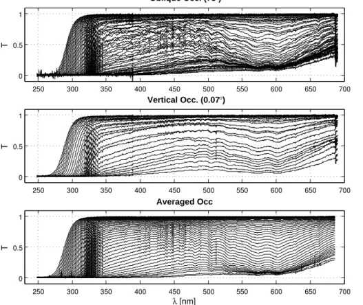
photometers (with 1 kHz sampling rate) were installed in parallel to the spectrometers. However, it appears that the correction of the scintillation is right when the star set-ting is vertical (close to the orbital plane) but imperfect for oblique occultations (Sofieva et al., 2009). In this case, residual scintillation persists due to atmospheric inhomo-geneous horizontal structures. Figure 1 shows an example of transmittance spectra

20

obtained from oblique (top panel) and vertical (middle panel) occultations. The pres-ence of residual scintillations is clearly visible in the spectra from oblique occultation whereas scintillation is almost perfectly removed in the spectra from vertical occulta-tion. The vertical resolution is 1.7 km for vertical occultations and better for oblique ones.

25

(7)

AMTD

6, 3511–3543, 2013

C. T ´etard et al.

Title Page

Tables Figures

◭ ◮

Back Close

Full Screen / Esc

Discussion

P

a

per

|

Dis

cussion

P

a

per

|

Discussion

P

a

per

|

Discussio

n

P

a

per

|

monitoring of stratospheric and mesospheric ozone. Furthermore, the large wavelength range and the spectral resolutions allows the retrieval of other species like NO₂, NO₃, H2O, O2, OClO and aerosol extinction (Bertaux et al., 2010). The following section

explains the method used to retrieve OClO.

3 The retrieval of OClO

5

The starting point of most occultation retrieval algorithm is the well-known Beer-Lambert law. It describes how the signal is affected by the presence of atmospheric absorbers along the line of sight at tangent altitude z:

S(λ,z) =S₀(λ) exp −

X

i

σ_i(λ)N_i(z)

!

(1)

where σ_i is the extinction cross-section and N_i is the slant column density of each

10

atmospheric absorbers in the spectral range selected. A detailed overview of the GO-MOS operational algorithm can be find in Kyr ¨ol ¨a et al. (2010b). Most of the expected species can be directly retrieved from single measurements but the combination of the weak signal-to-noise ratio of a single GOMOS measurement and the small optical thickness of OClO forces us to combine several single measurements in order to detect

15

it. The retrieval of OClO from GOMOS measurements requires two steps. The first is the calculation of an averaged transmittance spectra and the second is the inversion process of these spectra.

As written previously, the first step is required to increase the signal-to-noise ratio so that the retrieval of OClO can be carried out in the second step of the process. The

20

(8)

AMTD

6, 3511–3543, 2013

C. T ´etard et al.

Title Page

Tables Figures

◭ ◮

Back Close

Full Screen / Esc

Discussion

P

a

per

|

Dis

cussion

P

a

per

|

Discussion

P

a

per

|

Discussio

n

P

a

per

|

moment. For the selection of the GOMOS measurements used to build the averaged measurements, we have used the following steps:

– selection of stars: stars with effective temperatures greater than 4100 K to ensure a sufficient UV flux and stars with magnitudes lower than 2 to have acceptable photon fluxes. These criteria lead to a selection of 44 stars.

5

– temporal resolution: one month or one year. The time period is September 2002 to the end of 2011. The choice of this temporal bin size is influenced by the latitudinal resolution hereafter.

– latitude bands: for the annual climatologies, we have used 10◦_{latitude bands and} for the monthly time series, we have used 20◦ _{latitude bands for the regions}

lo-10

cated between−30◦ and+30◦ and 30◦ latitude bands elsewhere to ensure suffi

-cient numbers of measurements in each data set.

– illumination conditions: only dark limb and straylight condition measurements are used. Dark limb condition corresponds to measurements made when the solar zenith angle is higher than 120◦_{. These measurements are supposed to be used}

15

without restriction. Measurements are said to be in straylight conditions if the in-strument is illuminated by light coming from the scattering of solar light. Straylight measurements are considered as of good quality (more details can be found in the GOMOS product handbook at http://envisat.esa.int/handbooks/gomos/toc.htm).

– the GOMOS data used here are obtained with the version 5 of the ESA level 1

20

operational processor.

– all the selected spectra are linearly interpolated on a common vertical grid of tangent altitudes from 0 to 60 km with 1 km step.

Figure 2 shows the latitudinal distribution of the GOMOS data used in our study. A total number of about 162 000 GOMOS measurements has been processed. While

25

(9)

AMTD

6, 3511–3543, 2013

C. T ´etard et al.

Title Page

Tables Figures

◭ ◮

Back Close

Full Screen / Esc

Discussion

P

a

per

|

Dis

cussion

P

a

per

|

Discussion

P

a

per

|

Discussio

n

P

a

per

|

periods, the other latitudes are very well sampled during all years (except in 2005). During the first months of 2005 (until June), almost no measurements are available due to an instrumental breakdown. However, some measurements in the polar regions could be carried out (particularly in January).

For each bin, we have built a data set:

T1 λi,zj

, . . ., Tn λi,zj

wherezj are the 5

61 tangent altitude levels,λ_i are the wavelengths andnis the number of GOMOS mea-surements in the bin. Once all the data sets are built, they should be statistically ana-lyzed to guarantee the homogeneity of the bin data sets and subsequently, to ensure the representativity of the averaged measurement that will be derived from this data set. For each data set, statistical detections of multimodal distribution are performed

10

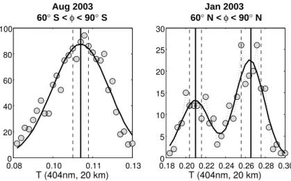
by fitting the distribution with theoretical models. Figure 3 shows examples of GOMOS transmittance distributions for a monomodal and a bimodal case. The bimodality ob-served here in the high latitude band is due to the fact that some measurements are inside the polar vortex and others are outside. In fact, transmittances inside the po-lar vortex are greater than those outside the popo-lar vortex because the decrease in

15

NO2 concentrations in the vortex area (denoxification) is not sufficiently offset by the

increase of OClO concentrations. All the cases of bimodal distributions observed in our study are due to measurements done inside and outside the polar vortex. In this case, both modes are studied separately and, after visual inspection, we have selected the one that represents the high latitude band, in other words the one inside the polar

20

vortex with greater transmittances (the other modes will be analyzed in the frame of some case studies). Then, an outlier detection is performed for each dataset using a jackknife method. Finally, for each tangent altitude and each wavelength, the weighted median transmittance is calculated. A weighted median calculation starts by sorting the transmittance values in increasing order, and rearranging the associated weights in the

25

(10)

AMTD

6, 3511–3543, 2013

C. T ´etard et al.

Title Page

Tables Figures

◭ ◮

Back Close

Full Screen / Esc

Discussion

P

a

per

|

Dis

cussion

P

a

per

|

Discussion

P

a

per

|

Discussio

n

P

a

per

|

of the absolute values of the difference between each transmittance values and the weighted median. This statistical study ensures that the calculated averaged spectra are representative of the considered region. Figure 1 shows transmittance spectra in the 250 to 690 nm range for a single oblique occultation, a single vertical occultation and an averaged occultation. We can note that the signs of residual scintillation

disap-5

pear in the averaged spectra (bottom panel) and that residual scintillations are almost perfectly corrected in the vertical occultation spectra (center panel) whereas some re-maining scintillations persist in the oblique spectra (top panel).

The second step consists of a Differential Optical Absorption Spectroscopy (DOAS) algorithm applied to averaged transmittance spectra to retrieve all the chemical species

10

involved in the absorption of the radiation in the wavelength range used. The DOAS technique has been reviewed by Platt et al. (1979). The principle of this method is quite simple: it is based on the idea that the transmittance consists of two compo-nents, one varying slowly with the wavelength and the other rapidly varying. In the spectral range used, the slowly varying componentTs(λ) reflects the Rayleigh

scatter-15

ing, aerosol extinction and the slowly varying part of the gaseous absorptions while the second component represents the rapidly varying part of gaseous absorptions.Ts(λ)

is obtained by fitting the measured transmittanceT(λ) by a second order polynomial in the wavelength window selected. Then, the experimental differential transmittance dT(λ) is simply expressed as the difference betweenT(λ) andTs(λ) while the modeled

20

differential transmittanceM(λ) is expressed as:

M(λ) =T_s

 exp

 −

X

j

N_gas_jδ σ_gas_j

 −1



 (2)

whereNgasj andδ σgasj correspond respectively to the SCD and the differential

cross-sections of the absorber gas in the wavelength interval. δ σgas_j is the difference

between the absorption cross-section of gas j and a first order polynomial fitting

25

(11)

AMTD

6, 3511–3543, 2013

C. T ´etard et al.

Title Page

Tables Figures

◭ ◮

Back Close

Full Screen / Esc

Discussion

P

a

per

|

Dis

cussion

P

a

per

|

Discussion

P

a

per

|

Discussio

n

P

a

per

|

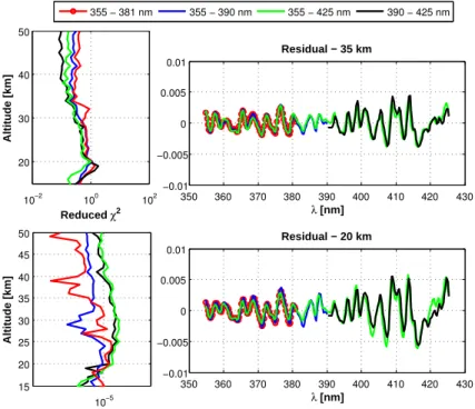
modeled and the experimental differential transmittances weighted by the measure-ment errors is applied for each tangent altitude to obtain the SCD of each species contributing to the absorption in the selected wavelength range and the retrieval errors (extracted from the jacobian matrix). We have studied 4 spectral ranges: 355–381 nm, 355–390 nm, 390–425 nm and 355–425 nm. For these 4 fitting windows, we have

cal-5

culated at each tangent altitudez_tthe reduced chi-squareχ2:

χ2(z_t) = 1

df

n

X

i=1

_{d T}₍_λ

i,zt)−M(λi,zt)

ǫ(λ_i,z_t)

2

. (3)

In this expression,nis the number of pixels in the fitting window,df is the degree of

freedom (nminus the number of parameters used in the minimization process) andǫis the error associated to the averaged differential transmittance. For the fitting windows

10

selected, the reduced chi-square are between about 0.1 and 1.5 (an example is pre-sented in the top left panel in Fig. 4). On the basis of this example, the best chi-square (χ2≈1) is obtained with the interval 355–381 nm for all the altitude range. Moreover,

the analysis of the mean of the residual (i.e. the difference between observed and mod-eled transmittances) at each tangent altitude shows that below 25 km there is almost

15

no differences but above, the mean residual is lower when the 355–381 nm wavelength range is used (bottom left panel in Fig. 4). Furthermore, residuals at each tangent al-titude (right panels in Fig. 4) are clearly smaller below 390 nm. The same study has been done using several other averaged occultations and the conclusions are always identical: we have therefore selected the 355–381 nm spectral window. In this

spec-20

tral range, we have to consider the absorptions of OClO, NO2 and also O3even if its

cross-section is very small in this range. Thus, these 3 species are fitted simultane-ously. In Fig. 5, we show an example of OClO SCDs in the Antarctic region (in blue), in the Arctic region (in black) and in the equatorial region (in red) for the year 2003. For OClO, the retrieval errors are generally better than 50 %. We can already notice

sev-25

(12)

AMTD

6, 3511–3543, 2013

C. T ´etard et al.

Title Page

Tables Figures

◭ ◮

Back Close

Full Screen / Esc

Discussion

P

a

per

|

Dis

cussion

P

a

per

|

Discussion

P

a

per

|

Discussio

n

P

a

per

|

in the equatorial regions and the expected chlorine activation in the lower stratosphere in both polar regions with a higher amplitude in the south.

The following section presents a preliminary validation of the OClO GOMOS product by comparisons with products retrieved using balloon-borne instruments.

4 Comparisons with other instruments

5

Since the nighttime OClO SCD from GOMOS averaged measurements is a new prod-uct, it is not easy to validate it. In this validation exercise, we have excluded O3 and

NO₂SCDs retrieved using the present algorithm because the spectral window used is not the most appropriate one to perform the retrieval of these species, considered here as interfering species. Nonetheless, as a first analysis of the quality of our products,

10

we can compare NO₂ retrieved from GOMOS averaged measurements and the oper-ational GOMOS data. This has been done previously and published in T ´etard et al. (2009). The results (not reproduced here) indicate that there is a very good agreement between both products (typically, relative differences are between−10 and 10 %) and

that our method seems to work properly.

15

The second step consists in comparing the GOMOS products with those from other instruments. The only nighttime OClO concentration profiles available for comparisons are those retrieved from the AMON and SALOMON balloon-borne instruments. One should keep in mind that these comparisons are done between spatially and tempo-rally localized measurements and a composite of several measurements localized in a

20

latitude band. AMON and SALOMON instruments performed nighttime remote sens-ing measurements ussens-ing respectively the stellar and the lunar occultation method. They provided slant column densities of OClO. However, since the observation geometries of GOMOS and of balloon-borne instruments are different, it is not appropriate to com-pare directly the slant column densities but instead should comcom-pare the OClO vertical

25

(13)

AMTD

6, 3511–3543, 2013

C. T ´etard et al.

Title Page

Tables Figures

◭ ◮

Back Close

Full Screen / Esc

Discussion

P

a

per

|

Dis

cussion

P

a

per

|

Discussion

P

a

per

|

Discussio

n

P

a

per

|

concentric layers that are assumed to be homogeneous. Using the matrix formalism, the problem consists of solving the following linear system:

N=K n (4)

where the matrix elements ofNare the OClO SCDs at each tangent altitude,Kis the kernel matrix (a triangular square matrix) and n is the OClO vertical profiles matrix.

5

The GOMOS spatial inversion is a well-conditioned problem and is easy to solve by using standard method.

AMON is a UV-visible spectrometer that uses the stellar occultation method. The flight used took place in March 2003 in Kiruna, northern Sweden (latitude 67◦₅₃′_N, longitude 21◦₀₅′_{E). We have used the measurements from the occultation of Sirius (}_α

10

Canis Majoris) and Alnilam (ǫOrionis). Both stars emit enough UV radiation to detect OClO (effective temperatures are respectively 11 000 and 30 000 K).

The second balloon-borne instrument used is SALOMON (Renard et al., 2000). It is a UV-visible spectrometer that uses the lunar occultation method. The flight occurred in January 2006 in Kiruna and the measurements were done during the balloon ascent

15

inside the polar vortex. The OClO concentration profile from the SALOMON measure-ments has been studied by comparisons with the results of the model described in Berthet et al. (2007). In particular, they have shown that OClO product from SALOMON is in an acceptable agreement with results from chemistry transport model calculations. For the inter-comparisons, the GOMOS measurements used to build the averaged

20

measurements were chosen located between 60◦_{and 75}◦ _{and took place in a 20 days} window centered on the flight date. Since the GOMOS vertical resolution is close to the AMON and SALOMON resolutions, no smoothing procedure was required and direct comparisons could be done.

Figure 6 shows the OClO concentration profiles comparisons. The curves on the left

25

(14)

AMTD

6, 3511–3543, 2013

C. T ´etard et al.

Title Page

Tables Figures

◭ ◮

Back Close

Full Screen / Esc

Discussion

P

a

per

|

Dis

cussion

P

a

per

|

Discussion

P

a

per

|

Discussio

n

P

a

per

|

the AMON (ǫ-ORI) profiles but is higher for the AMON (α-CMA) profile: 5.3×107cm−3,

5×107cm−3 and 1×108cm−3 respectively. The differences in concentration could be

explained by asserting that the OClO concentrations can vary according to the area of the vortex observed. A secondary maximum is observed in the three profiles at almost the same altitudes: 26 km for GOMOS and AMON (ǫ-ORI) and 26.5 km for AMON

5

(α-CMA). Here again, the concentration values reached are almost identical for the GOMOS and the AMON (ǫ-ORI) profiles (respectively 1.6×107 and 1.8×107cm−3)

whereas the AMON (α-CMA) profile exhibits a higher value: 2.5×107cm−3. Overall,

the OClO profile from the GOMOS averaged measurement is closer to the product of AMON whenǫ-ORI is occulted: for the entire altitude range, the AMON (ǫ-ORI) profiles

10

are well within the GOMOS error bars.

Concerning the comparisons with SALOMON (right panel of Fig. 6), the agreement is moderate. The first maximum is reached at about 20 km for SALOMON and at 18 km for GOMOS. This difference may not be significant because of the vertical resolu-tion of SALOMON for this product (2 km). However, the maximum of OClO

concen-15

tration measured by SALOMON is twice the one retrieved by GOMOS (1.2×108 and

6.1×107cm−3 respectively). Moreover, above 28 km, the SALOMON concentrations

increase strongly reaching a value of 1.3×108cm−3at 32 km whereas the OClO

con-centrations from GOMOS are always decreasing.

In summary, the OClO product from GOMOS averaged measurements compares

20

(15)

AMTD

6, 3511–3543, 2013

C. T ´etard et al.

Title Page

Tables Figures

◭ ◮

Back Close

Full Screen / Esc

Discussion

P

a

per

|

Dis

cussion

P

a

per

|

Discussion

P

a

per

|

Discussio

n

P

a

per

|

5 Climatology of OClO

5.1 Annual climatology

As specified previously, we use 10◦_{latitude bins for the annual climatologies. For each} altitude, the distribution of OClO SCDs with latitude are fitted by one or two lorentzian function(s), taking into account the retrieval errors.

5

In Fig. 7, we present the isopleths of the latitude-altitude OClO slant column densi-ties (log scales) for years 2003 to 2011. The altitude range is limited from 15 to 45 km. Outside this range, either the retrieval does not succeed or the uncertainties of the retrieval are too large. The 9 latitude-altitude maps of OClO SCDs presented in Fig. 7 show approximately the same structure. In the lower stratosphere, we can observe

10

high values in the polar regions, reaching about 1016cm−2_{in the southern hemisphere} and generally slightly less in the north (about 1015cm−2_{). These high values are} ex-pected (Eq. R1) and are an indication of the chlorine activation that occurs in spring (in the northern hemisphere) and in fall (in the southern hemisphere). At higher alti-tude in the polar regions, OClO SCDs decrease abruptly for all years. This decrease

15

can be explained by the scarcity of ClO at these altitudes. This is well observed by the Microwave Limb Sounder (MLS) instrument onboard the satellite platform AURA (see plots available at http://mls.jpl.nasa.gov).

In the equatorial region, an OClO layer is present all year between about 30 to 35 km. The latitudinal extent as well as the maxima of the layer is somewhat variable from one

20

year to another. The fact remains that the maxima are about a few 1014cm−2_{. The} location of the maxima is approximately around the equator. Note that the year 2011 exhibits the stronger OClO equatorial layer (the maxima is nearly 1015cm−2_{). The OClO} equatorial stratospheric layer was first discovered by Fussen et al. (2006) for the year 2003. A possible explanation for the presence of OClO at these altitudes can be the low

25

pressure at these levels which make the 3 body reactions between ClO/BrO and NO2

(16)

AMTD

6, 3511–3543, 2013

C. T ´etard et al.

Title Page

Tables Figures

◭ ◮

Back Close

Full Screen / Esc

Discussion

P

a

per

|

Dis

cussion

P

a

per

|

Discussion

P

a

per

|

Discussio

n

P

a

per

|

MLS confirms the presence of a ClO layer in the upper stratosphere in the equatorial region. One may notice the more extended (in terms of altitude) OClO layers for the years 2008 and 2011. Finally, the OClO SCDs decrease progressively above this layer. The other latitude regions are characterized by weak OClO values. Consequently, in the following, our attention will be focused on equatorial and polar regions.

5

5.2 Monthly climatology of OClO

In Fig. 8, we show the time series of OClO SCDs in three latitude bands: the equatorial band (10◦_S–10◦_{N, middle panel), the north polar band (60}◦_N–90◦_{N, top panel) and} the south polar band (60◦_S–90◦_{S, bottom panel). In the equatorial region, the missing} data in 2005 are due to a GOMOS failure. The discontinuity observed in the two polar

10

time series are due to the spatial coverage of GOMOS at these altitudes (cf. Fig. 2). Regarding the northern latitude band, we can clearly observe an annual increase of OClO followed by a decrease in the lower stratosphere (below about 25 km). The increase begins in December and reaches a maximum of about 5×1015cm−2 to

3×1016cm−2. The corresponding OClO concentrations (obtained after the spatial

in-15

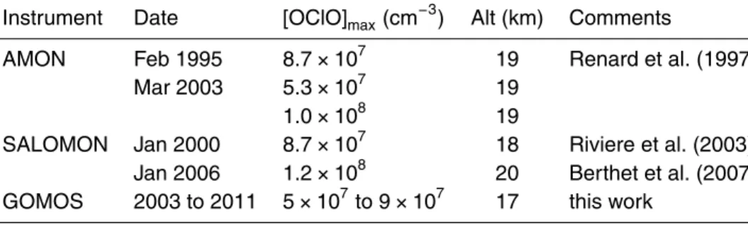
version described in Sect. 4) are 5×107 to 9×107cm−3. This is in good agreement

with the values previously observed with other instruments (summarized in Table 1). Regarding the altitude of the maximum of OClO concentrations, the values obtained using GOMOS measurements (about 17 km) are generally lower than those found by the balloon-borne instruments. The high OClO values are the sign of chlorine

activa-20

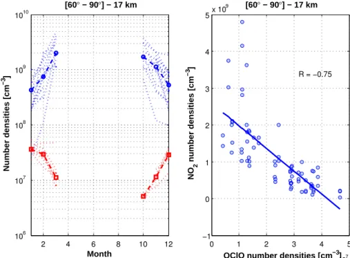
tion in the winter polar vortex. Note that the year 2011 shows strong OClO values in the lower stratosphere. Indeed, the ozone depletion in the Arctic winter 2010/2011 has been one of the most important of the last decade (Kuttippurath et al., 2012). This fea-ture is also observed in the corresponding annual isopleth (Fig. 7). Figure 9 shows the anti-correlation plot between OClO and NO2concentrations (from the GOMOS

opera-25

(17)

AMTD

6, 3511–3543, 2013

C. T ´etard et al.

Title Page

Tables Figures

◭ ◮

Back Close

Full Screen / Esc

Discussion

P

a

per

|

Dis

cussion

P

a

per

|

Discussion

P

a

per

|

Discussio

n

P

a

per

|

The correlation coefficient obtained is about−0.75 which confirms the anti-correlation

between NO₂ and OClO. Indeed, during the permanent polar night, NO₂ is remove from the stratosphere because of Reactions (R4) and (R5). Therefore, the reaction of formation of OClO (Reaction R1) is more active.

For the south polar region (bottom panel in Fig. 8), only a few months of each year

5

can be analyzed (from July to September). Typically, the time series shows high OClO values from July to September indicating the sign of chlorine activation. The OClO SCD maximum reached in the Antarctic regions (from 1.5_×1016 to 5.7_×1016cm−2_{) are} larger than those observed in the Arctic regions. This is well illustrated in Fig. 10 show-ing these OClO SCD maxima for winters 2003 to 2011. The maximum concentrations

10

range from 7_×107cm−3_{to 2}

×108cm−3. Unfortunately, we can not validate our values

because of the lack of occultation measurements in the south pole.

The equatorial region (middle panel in Fig. 8) is characterized by an OClO layer between about 30 to 40 km for each year. There are too few values available in 2005 to discuss this year. In this layer, the maximum is located at about 35 km for the years

15

2003, 2006, 2007 and 2009 to 2011. For the years 2004 and 2008, the maximum is located slightly lower, around 32 km. This layer appears to be present during the entire year with only small variations.This is in good agreement with the results obtained by the MLS instrument which shows a quasi-constant ClO layer at these altitudes with a volume mixing ratio of 0.3 to 0.4 ppbv, corresponding to concentrations of 2×107 to

20

3×107cm−3. Note that a stronger OClO layer is observed for periods ranging from

(18)

AMTD

6, 3511–3543, 2013

C. T ´etard et al.

Title Page

Tables Figures

◭ ◮

Back Close

Full Screen / Esc

Discussion

P

a

per

|

Dis

cussion

P

a

per

|

Discussion

P

a

per

|

Discussio

n

P

a

per

|

6 Conclusions

In this article, we have presented an innovative method to retrieve small absorber con-centration. This method is applied to the GOMOS measurements to detect OClO. It consists of the combination of several co-located GOMOS measurements to build one measurement with a higher signal-to-noise ratio. Then a specified algorithm is used to

5

retrieve OClO slant column densities.

We have compared our results with those obtained using balloon-borne instruments AMON and SALOMON. It appears that our OClO product is in a very good agreement with the AMON product and compares slightly less well with SALOMON.

We have constructed climatologies of OClO based on annual binning. It appears

10

clearly that the same structures emerge every year. First, in the polar regions, we systematically observed a strong increase of OClO in the lower stratosphere. This is related to the activation of the chlorine species in the polar vortex. Moreover, an OClO layer in the equatorial region is clearly detected each year in the middle stratosphere. This layer is the result of the reaction between BrO and ClO effectively detected at

15

these altitudes by the MLS instrument.

Time series of OClO SCDs have been built using averaged measurements repre-sentative of one month for three latitude bands corresponding to Arctic, Antarctic and equatorial regions. The period of these climatologies is from 2003 to 2012, covering the entire GOMOS mission. It appears that activation of chlorine species is well observed

20

in the winter pole. Furthermore, the OClO layer in the equatorial middle stratosphere is detected during all the years studied and presents no particular variations. The anti-correlation between OClO and NO2concentrations is well observed.

The next step of these studies will be the use of models to interpret quantitatively the results presented in this article. The method presented here is really promising

25

(19)

AMTD

6, 3511–3543, 2013

C. T ´etard et al.

Title Page

Tables Figures

◭ ◮

Back Close

Full Screen / Esc

Discussion

P

a

per

|

Dis

cussion

P

a

per

|

Discussion

P

a

per

|

Discussio

n

P

a

per

|

considered as the first and only long-term nighttime OClO climatology that exists at present.

Acknowledgements. This study was funded by the PRODEX/RADIAL (PEA 4000102793) con-tract under the authority of the Belgian Space Science O_ffice (BELSPO).

We thank the AMON and SALOMON science team for giving us the authorization to use their 5

OClO concentration profiles.

References

Bertaux, J. L., Pellinen, R., Simon, P., Chassefi ère, E., Dalaudier, F., Godin, S., Goutail, F., Hauchecorne, A., Le Texier, H., M égie, G., Pommereau, J. P., Brasseur, G., Kyr öl ä, E., Tuomi, T., Korpela, S., Leppelmeier, G., Visconti, G., Fabian, P., Isaksen, S. A., Larsen, S. H., Stor-10

dahl, F., Cariolle, D., Lenoble, J., Naudet, J. P., and Scott, N.: GOMOS, proposal in response to ESA EPOP-1, A.O.1, January 1988. 3516

Bertaux, J. L., Kyr öl ä, E., Fussen, D., Hauchecorne, A., Dalaudier, F., Sofieva, V., Tamminen, J., Vanhellemont, F., Fanton d’Andon, O., Barrot, G., Mangin, A., Blanot, L., Lebrun, J. C., P érot, K., Fehr, T., Saavedra, L., Leppelmeier, G. W., and Fraisse, R.: Global ozone monitoring by 15

occultation of stars: an overview of GOMOS measurements on ENVISAT, Atmos. Chem. Phys., 10, 12091–12148, doi:10.5194/acp-10-12091-2010, 2010. 3514, 3517

Berthet, G., Renard, J. B., Catoire, V., Chartier, M., Robert, C., Huret, N., Coquelet, F., Bour-geois, Q., Riviere, E. D., Barret, B., Lefevre, F., and Hauchecorne, A.: Remote sensing mea-surements in the polar vortex: comparison to in situ observations and implications for the 20

simultaneous retrievals and analysis of the NO₂and OClO species, J. Geophys. Res., 112, D21310, doi:10.1029/2007JD008699, 2007. 3514, 3523, 3533

Damiani, A., Funke, B., Marsh, D. R., L ´opez-Puertas, M., Santee, M. L., Froidevaux, L., Wang, S., Jackman, C. H., von Clarmann, T., Gardini, A., Cordero, R. R., and Storini, M.: Impact of January 2005 solar proton events on chlorine species, Atmos. Chem. Phys. Discuss., 12, 25

1935–1978, doi:10.5194/acpd-12-1935-2012, 2012.

(20)

AMTD

6, 3511–3543, 2013

C. T ´etard et al.

Title Page

Tables Figures

◭ ◮

Back Close

Full Screen / Esc

Discussion

P

a

per

|

Dis

cussion

P

a

per

|

Discussion

P

a

per

|

Discussio

n

P

a

per

|

Fussen, D., Vanhellemont, F., Dodion, J., Bingen, C., Mateshvili, N., Daerden, F., Fonteyn, D., Errera, Q., Chabrillat, S., Kyr ¨ol ¨a, E., Tamminen, J., Sofieva, V., Hauchecorne, A., Dalaudier, F., Bertaux, J.-L., Renard, J.-B., Fraisse, R., d’Andon, O. F., Barrot, G., Guirlet, M., Man-gin, A., Fehr, T., Snoeij, P., and Saavedra, L.: A global OClO stratospheric layer dis-covered in GOMOS stellar occultation measurements, Geophys. Res. Lett., 33, L13815, 5

doi:10.1029/2006GL026406, 2006. 3515, 3525

Hauchecorne, A., Bertaux, J.-L., Dalaudier, F., Russel III, J. M., Mlynczak, M. G., Kyr ¨ol ¨a, E., and Fussen, D.: Large increase of NO₂in the north polar mesosphere in January–February 2004: Evidence of a dynamical origin from GOMOS ENVISAT and SABER TIMED data, Geophys. Res. Lett., 34, L03810, doi:10.1029/2006GL027628, 2007.

10

Krecl, P., Haley, C. S., Stegman, J., Brohede, S. M., and Berthet, G.: Retrieving the vertical distribution of stratospheric OClO from Odin/OSIRIS limb-scattered sunlight measurements, Atmos. Chem. Phys., 6, 1879–1894, doi:10.5194/acp-6-1879-2006, 2006. 3514

K ¨uhl, S., Pukite, J., Deutschmann, T., Platt, U., and Wagner, T.: SCIAMACHY limb measure-ments of NO₂, BrO and OClO, Retrieval of vertical profiles: Algorithm, first results, sensitivity 15

and comparison studies, Adv. Space Res., 42, 1747–1764, 2008. 3514

Kuttippurath, J., Godin-Beekmann, S., Lef `evre, F., Nikulin, G., Santee, M. L., and Froidevaux, L.: Record-breaking ozone loss in the Arctic winter 2010/2011: comparison with 1996/1997, Atmos. Chem. Phys., 12, 7073–7085, doi:10.5194/acp-12-7073-2012, 2012. 3526

Kyr ¨ol ¨a, E., Tamminen, J., Sofieva, V., Bertaux, J. L., Hauchecorne, A., Dalaudier, F., Fussen, 20

D., Vanhellemont, F., Fanton d’Andon, O., Barrot, G., Guirlet, M., Fehr, T., and Saavedra de Miguel, L.: GOMOS O₃, NO₂, and NO₃ observations in 2002–2008, Atmos. Chem. Phys., 10, 7723–7738, doi:10.5194/acp-10-7723-2010, 2010a.

Kyr ¨ol ¨a, E., Tamminen, J., Sofieva, V., Bertaux, J. L., Hauchecorne, A., Dalaudier, F., Fussen, D., Vanhellemont, F., Fanton d’Andon, O., Barrot, G., Guirlet, M., Mangin, A., Blanot, L., Fehr, T., 25

Saavedra de Miguel, L., and Fraisse, R.: Retrieval of atmospheric parameters from GOMOS data, Atmos. Chem. Phys., 10, 11881–11903, doi:10.5194/acp-10-11881-2010, 2010b. 3517 Miller, H. L. J., Sanders, R. W., and Solomon, S.: Observations and interpretation of column OClO seasonal cycles at two polar sites, J. Geophys. Res., 104, 18769–18783, 1999. 3514 Oetjen, H., Wittrock, F., Richter, A., Chipperfield, M. P., Medeke, T., Sheode, N., Sinnhuber, 30

(21)

AMTD

6, 3511–3543, 2013

C. T ´etard et al.

Title Page

Tables Figures

◭ ◮

Back Close

Full Screen / Esc

Discussion

P

a

per

|

Dis

cussion

P

a

per

|

Discussion

P

a

per

|

Discussio

n

P

a

per

|

Platt, U., Perner, D., and P ¨atz, H. W.: Simultaneous measurement of atmospheric CH₂O, O₃, and NO₂ by differential optical absorption, J. Geophys. Res., 84, 6329–6335, doi:10.1029/JC084iC10p06329, 1979. 3520

Renard, J. B., Lefevre, F., Pirre, M., Robert, C., and Huguenin, D.: Vertical profile of night-time stratospheric OClO, J. Atmos. Chem., 26, 65–76, 1997. 3514, 3533

5

Renard, J. B., Chartier, M., Robert, C., Chalumeau, G., Berthet, G., Pirre, M., and Pommereau, J. P.: SALOMON: a new, light, balloon-borne UV visible spectrometer for nighttime observa-tions of stratospheric trace gas species, Appl. Optics, 39, 386–392, 2000. 3514, 3523 Renard, J.-B., Blelly, P.-L., Bourgeois, Q., Chartier, M., Goutail, F., and Orsolini, Y.-J.: Origin

of the January–April 2004 increase in stratospheric NO2 observed in the northern polar 10

latitudes, Geophys. Res. Lett., 33, L11801, doi:10.1029/2005GL025450, 2006.

Riviere, E. D., Pirre, M., Berthet, G., Renard, J. B., Taupin, F. G., Huret, N., and Chartier, M.: On the interaction between nitrogen and halogen species in the Arctic polar vortex during THESEO and THESEO 2000, J. Geophys. Res., 108, 8311, doi:10.1029/2002JD002087, 2003. 3514, 3533

15

Riviere, E. D., Pirre, M., Berthet, G., Renard, J. B., and Lefevre, F.: Investigating the halogen chemistry from the high-latitude nighttime stratospheric measurements of OClO and NO₂, J. Atmos. Chem., 48, 261–282, 2004. 3514

Rusch, D. W., G ´erard, J. C., and Solomon, S.: The effect of particle precipitation events on the neutral and ion chemistry of the middle atmosphere – I. Odd nitrogen, Planet. Space Sci., 20

29, 767–774, 1981.

Salawitch, R. J., Wofsy, S. C., Gottlieb, E. W., Lait, L. R., Newman, P. A., Schoeberl, M. R., Loewenstein, M., Podolske, J. R., Strahan, S. E., and Proffitt, M. H.: Chemical loss of ozone in the Arctic polar vortex in the winter of 1991–1992, Science, 261, 1146–1149, doi:10.1126/science.261.5125.1146, 1993. 3513

25

Sepp äl ä, A., Veronen, P. T., Kyr öl ä, E., Hassinen, S., Backman, L., Hauchecorne, A., Bertaux, J. L., and Fussen, D.: Solar proton events of October–November 2003: Ozone depletion in the northern hemisphere polar winter as seen by GOMOS/Envisat, Geophys. Res. Lett., 31, L19107, doi:10.1029/2004GL021042, 2004.

Sofieva, V. F., Kan, V., Dalaudier, F., Kyr ¨ol ¨a, E., Tamminen, J., Bertaux, J.-L., Hauchecorne, A., 30

(22)

AMTD

6, 3511–3543, 2013

C. T ´etard et al.

Title Page

Tables Figures

◭ ◮

Back Close

Full Screen / Esc

Discussion

P

a

per

|

Dis

cussion

P

a

per

|

Discussion

P

a

per

|

Discussio

n

P

a

per

|

Solomon, S.: Stratospheric ozone depletion: A review of concepts and history, Rev. Geophys., 37, 275–316, doi:10.1029/1999RG900008, 1999. 3514

Solomon, S., Garcia, R. R., Rowland, F. S., and Wuebbles, D. J.: On the depletion of antarctic ozone, Nature, 321, 755–758, 1986. 3513

Solomon, S., Mount, G. H., and Sanders, R.W. Schmeltekopf, A. L.: Visible spectroscopy at 5

McMurdo station, Antartica 2. Observations of OClO, J. Geophys. Res., 92, 8329–8338, 1987. 3514

T étard, C., Fussen, D., Bingen, C., Capouillez, N., Dekemper, E., Loodts, N., Mateshvili, N., Vanhellemont, F., Kyr öl ä, E., Tamminen, J., Sofieva, V., Hauchecorne, A., Dalaudier, F., Bertaux, J.-L., Fanton d’Andon, O., Barrot, G., Guirlet, M., Fehr, T., and Saavedra, L.: Si-10

multaneous measurements of OClO, NO₂ and O₃in the Arctic polar vortex by the GOMOS instrument, Atmos. Chem. Phys., 9, 7857–7866, doi:10.5194/acp-9-7857-2009, 2009. 3514, 3515, 3522

Wagner, T., Wittrock, F., Richter, A., Wenig, M., and Burrows, J. P., and Platt, U.: Continuous monitoring of the high and persistent chlorine activation during the Arctic winter 1999/2000 by 15

(23)

AMTD

6, 3511–3543, 2013

C. T ´etard et al.

Title Page

Tables Figures

◭ ◮

Back Close

Full Screen / Esc

Discussion

P

a

per

|

Dis

cussion

P

a

per

|

Discussion

P

a

per

|

Discussio

n

P

a

per

|

Table 1.Maximum of OClO concentrations previously detected by balloon-borne instruments during nighttime in the Arctic polar vortex. The altitude of the maximum is also indicated.

Instrument Date [OClO]_max(cm−3₎ _{Alt (km)} _Comments

AMON Feb 1995 8.7×107 19 Renard et al. (1997)

Mar 2003 5.3×107 19

1.0×108 19

SALOMON Jan 2000 8.7×107 18 Riviere et al. (2003)

Jan 2006 1.2×108 20 Berthet et al. (2007)

(24)

AMTD

6, 3511–3543, 2013

C. T ´etard et al.

Title Page

Tables Figures

◭ ◮

Back Close

Full Screen / Esc

Discussion

P

a

per

|

Dis

cussion

P

a

per

|

Discussion

P

a

per

|

Discussio

n

P

a

per

|

JAN2003 JAN2004 JAN2005 JAN2006 JAN2007 JAN2008 JAN2009 JAN2010 JAN2011 JAN2012 −100

−80 −60 −40 −20 0 20 40 60 80 100

φ

[

°

]

(25)

AMTD

6, 3511–3543, 2013

C. T ´etard et al.

Title Page

Tables Figures

◭ ◮

Back Close

Full Screen / Esc

Discussion

P

a

per

|

Dis

cussion

P

a

per

|

Discussion

P

a

per

|

Discussio

n

P

a

per

|

0.080 0.10 0.11 0.13

20 40 60 80 100

T (404nm, 20 km) Aug 2003 60° S < φ < 90° S

0.18 0.20 0.22 0.24 0.26 0.28 0.300

5 10 15 20 25 30

T (404nm, 20 km) Jan 2003 60° N < φ < 90° N

(26)

AMTD

6, 3511–3543, 2013

C. T ´etard et al.

Title Page

Tables Figures

◭ ◮

Back Close

Full Screen / Esc

Discussion

P

a

per

|

Dis

cussion

P

a

per

|

Discussion

P

a

per

|

Discussio

n

P

a

per

|

Oblique Occ. (75°)

T

250 300 350 400 450 500 550 600 650 700 0

0.5 1

Vertical Occ. (0.07°)

T

250 300 350 400 450 500 550 600 650 700 0

0.5 1

Averaged Occ

λ [nm]

T

250 300 350 400 450 500 550 600 650 700 0

0.5 1

(27)

AMTD

6, 3511–3543, 2013

C. T ´etard et al.

Title Page

Tables Figures

◭ ◮

Back Close

Full Screen / Esc

Discussion

P

a

per

|

Dis

cussion

P

a

per

|

Discussion

P

a

per

|

Discussio

n

P

a

per

|

10−2 100 102

20 30 40 50

Reduced χ2

Altitude [km]

10−5

15 20 25 30 35 40 45 50

mean(residual)

Altitude [km]

350 360 370 380 390 400 410 420 430

−0.01 −0.005 0 0.005 0.01

Residual − 35 km

λ [nm]

350 360 370 380 390 400 410 420 430

−0.01 −0.005 0 0.005 0.01

Residual − 20 km

λ [nm]

355 − 381 nm 355 − 390 nm 355 − 425 nm 390 − 425 nm

(28)

AMTD

6, 3511–3543, 2013

C. T ´etard et al.

Title Page

Tables Figures

◭ ◮

Back Close

Full Screen / Esc

Discussion

P

a

per

|

Dis

cussion

P

a

per

|

Discussion

P

a

per

|

Discussio

n

P

a

per

|

1013 1014 1015 1016 1017

15 20 25 30 35 40 45

OClO SCD [cm−2 ]

Altitude [km]

[70° ; 80°S]

[0° ; 10°N]

[70° ; 80°N]

(29)

AMTD

6, 3511–3543, 2013

C. T ´etard et al.

Title Page

Tables Figures

◭ ◮

Back Close

Full Screen / Esc

Discussion

P

a

per

|

Dis

cussion

P

a

per

|

Discussion

P

a

per

|

Discussio

n

P

a

per

|

0 0.5 1 1.5 2 2.5

x 108

12 14 16 18 20 22 24 26 28 30 32

OClO concentration [cm−3]

Altitude [km]

SALOMON − Jan 2006 − North pole

0 5 10

x 107

16 18 20 22 24 26 28 30 32

AMON − Mar 2003 − North pole

OClO concentration [cm−3]

Altitude [km]

(30)

AMTD

6, 3511–3543, 2013

C. T ´etard et al.

Title Page Abstract Introduction Conclusions References Tables Figures ◭ ◮ ◭ ◮ Back Close

Full Screen / Esc

Printer-friendly Version Interactive Discussion Discussion P a per | Dis cussion P a per | Discussion P a per | Discussio n P a per |

−50 0 50

20 30 40 2003 h [km] 13.6 13.9 13.9 13.9 14.2 14.2 14.2 14.5 14.5 14.5 14.8 14.8 15.1 15.1 15.4 16

−50 0 50

20 30 40 2004 13.6 13.9 13.9 14.2 14.2 14.2 14.5 14.5 14.5 14.8 14.8 15.1 15.1 15.4 15.4

−50 0 50

20 30 40 2005 13 13 13.3 13.3 13.6 13.6 13.9 13.9 13.9 14.2 14.2 14.5 14.5 14.8 14.8 15.1 15.1 15.4 16

−50 0 50

20 30 40 2006 h [km] 13.3 13.3 13.6 13.6 13.914.2 14.2 14.2 14.5 14.5 14.5 14.8 15.1 15.4 15.4 15.7 16

−50 0 50

20 30 40 2007 13.6 13.6 13.9 14.2 14.2

14.5 14.5 14.5

14.5 14.8 15.1 15.1 15.4 16

−50 0 50

20 30 40 2008 13.9 14.2 14.5 14.5 14.5 14.8 14.8 14.8 15.1

15.1 15.4

16

−50 0 50

20 30 40

2009

φ [°]

h [km]

13.613.9 13.6

13.9 13.9 14.2 14.2 14.2 14.5 14.5 14.8 14.8 15.1

−50 0 50

20 30 40

2010

φ [°]

13.3 13.6 13.9 13.6

13.9 13.9 14.2 14.2 14.2 14.2 14.5 14.5 14.5 14.8 14.8

15.1 15.1_15.4

16

−50 0 50

20 30 40

2011

φ [°] 13.9 14.2 14.2 14.5 14.5 14.5 14.5 14.8 14.8 14.8 15.1 15.1 15.4 _15.4 16 16 13 13.5 14 14.5 15 15.5 16 16.5

Fig. 7.Latitude-altitude maps of OClO slant column densities (log scale, cm−2

(31)

AMTD

6, 3511–3543, 2013

C. T ´etard et al.

Title Page

Tables Figures

◭ ◮

Back Close

Full Screen / Esc

Discussion

P

a

per

|

Dis

cussion

P

a

per

|

Discussion

P

a

per

|

Discussio

n

P

a

per

|

Time (years)

h [km]

2003 2004 2005 2006 2007 2008 2009 2010 2011 20

30 40

13 14 15 16

h [km]

15 20 25 30 35 40 45

14 14.5 15

h [km]

Log₁₀ (N_OClO [cm−2])

20 30 40

13 14 15 16

Fig. 8.Monthly OClO slant column densities (cm−2

) in three latitude bands for the period from September 2002 to December 2011. Latitude bands: 60◦_N–90◦_{N (top panel), 10}◦_S–10◦_N

(mid-dle panel) and 60◦_S–90◦_{S (bottom panel). The colorscales used are the same for the two polar}

(32)

AMTD

6, 3511–3543, 2013

C. T ´etard et al.

Title Page

Tables Figures

◭ ◮

Back Close

Full Screen / Esc

Discussion

P

a

per

|

Dis

cussion

P

a

per

|

Discussion

P

a

per

|

Discussio

n

P

a

per

|

2 4 6 8 10 12

106

107

108

109

1010

[60° − 90°] − 17 km

Month

Number densities [cm

−3

]

0 1 2 3 4 5

x 107

−1 0 1 2 3 4

5x 10

9 [60° − 90°] − 17 km

OClO number densities [cm−3]

NO

2

number densities [cm

−3

]

R = −0.75

Fig. 9.Left panel: time series of monthly concentrations (molec cm−3_{) of OClO (red) and NO}

2 (blue) in the 60◦_–90◦_{latitude band for the year 2003 to 2011. The solid lines are the median}

con-centrations. Right panel: Correlation plot of concentrations of OClO versus NO₂(molec cm−3₎

(33)

AMTD

6, 3511–3543, 2013

C. T ´etard et al.

Title Page

Tables Figures

◭ ◮

Back Close

Full Screen / Esc

Discussion

P

a

per

|

Dis

cussion

P

a

per

|

Discussion

P

a

per

|

Discussio

n

P

a

per

|

Oct Nov Dec Jan Feb Mar 0

1 2 3 4 5 6x 10

16

Month

OClO

MAX

SCD [cm

−2

] 2002/2003

2003/2004 2004/2005 2005/2006 2006/2007 2007/2008 2008/2009 2009/2010 2010/2011

Antarctic (shifted by 6 months)

Arctic