A 6-year global climatology of occurrence of upper-tropospheric ice supersaturation inferred from the Atmospheric Infrared Sounder after synergetic calibration with MOZAIC

(1)

ACPD

11, 12889–12947, 2011

Ice supersaturation from the Atmospheric

InfraRed Sounder

N. Lamquin et al.

Title Page

Abstract Introduction

Conclusions References

Tables Figures

◭ ◮

Back Close

Full Screen / Esc

Printer-friendly Version Interactive Discussion

Discussion

P

a

per

|

Dis

cussion

P

a

per

|

Discussion

P

a

per

|

Discussio

n

P

a

per

|

Atmos. Chem. Phys. Discuss., 11, 12889–12947, 2011 www.atmos-chem-phys-discuss.net/11/12889/2011/ doi:10.5194/acpd-11-12889-2011

Atmospheric Chemistry and Physics Discussions

This discussion paper is/has been under review for the journal Atmospheric Chemistry and Physics (ACP). Please refer to the corresponding final paper in ACP if available.

A 6-year global climatology of occurrence

of upper-tropospheric ice supersaturation

inferred from the Atmospheric Infrared

Sounder after synergetic calibration with

MOZAIC

N. Lamquin1, C. J. Stubenrauch1, K. Gierens2, U. Burkhardt2, and H. Smit3

1

Laboratoire de M ´et ´eorologie Dynamique, UMR8539, CNRS/IPSL – Ecole Polytechnique, Palaiseau, France

2

Deutsches Zentrum f ¨ur Luft- und Raumfahrt, Oberpfaffenhofen, Germany 3

Forschungzentrum J ülich, Institut f ür Chemie der belasteten Atmosph äre (ICG2), J ülich, Germany

Received: 9 September 2010 – Accepted: 7 April 2011 – Published: 27 April 2011

Correspondence to: N. Lamquin (nicolas.lamquin@lmd.polytechnique.fr)

Published by Copernicus Publications on behalf of the European Geosciences Union.

(2)

ACPD

11, 12889–12947, 2011

N. Lamquin et al.

Title Page

Tables Figures

◭ ◮

Back Close

Full Screen / Esc

Discussion

P

a

per

|

Dis

cussion

P

a

per

|

Discussion

P

a

per

|

Discussio

n

P

a

per

|

Abstract

Ice supersaturation in the upper troposphere is a complex and important issue for the understanding of cirrus cloud formation. Infrared sounders have the ability to provide cloud properties and atmospheric profiles of temperature and humidity. On the other hand, they su_ffer from coarse vertical resolution, especially in the upper troposphere

5

and therefore are unable to detect shallow ice supersaturated layers. We have used data from the Measurements of OZone and water vapour by AIrbus in-service airCraft experiment (MOZAIC) in combination with Atmospheric InfraRed Sounder (AIRS) rel-ative humidity measurements and cloud properties to develop a calibration method for an estimation of occurrence frequencies of ice supersaturation. This method first

10

determines the occurrence probability of ice supersaturation, detected by MOZAIC, as a function of the relative humidity determined by AIRS. The occurrence probability function is then applied to AIRS data, independently of the MOZAIC data, to provide a global climatology of upper-tropospheric ice supersaturation occurrence. Our cli-matology is then related to high cloud occurrence from the Cloud-Aerosol Lidar with

15

Orthogonal Polarization (CALIOP) and compared to ice supersaturation occurrence statistics from MOZAIC alone. Finally it is compared to model climatologies of ice su-persaturation from the Integrated Forecast System (IFS) of the European Centre for Medium-Range Weather Forecasts (ECMWF) and from the European Centre HAm-burg Model (ECHAM). All the comparisons show good agreements when considering

20

the limitations of each instrument and model. This study highlights the benefits of multi-instrumental synergies for the investigation of upper tropospheric ice supersaturation.

1 Introduction

Ice supersaturation (or “ISS”, relative humidity with respect to ice larger than 100%) is a prerequisite for the nucleation of cirrus clouds (e.g. Haag et al., 2003) and for the

per-25

(3)

ACPD

11, 12889–12947, 2011

N. Lamquin et al.

Title Page

Tables Figures

◭ ◮

Back Close

Full Screen / Esc

Discussion

P

a

per

|

Dis

cussion

P

a

per

|

Discussion

P

a

per

|

Discussio

n

P

a

per

|

a parametrization of supersaturation despite the growing necessity of a better repre-sentation of ice cloud formation processes (Waliser et al., 2009). While radiosounding and in situ measurements provide measurements of relative humidity at a high vertical resolution (Spichtinger et al., 2003a; Kr ¨amer et al., 2009), continuous and global ob-servations are only achievable from satellite measurements which, in turn, su_ffer from

5

a limited vertical resolution.

For example, Kahn et al. (2008) and Lamquin et al. (2008) have shown that cirrus clouds have generally a smaller vertical extent (about 2 km) than the AIRS vertical res-olution (>3 km in the upper troposphere, Maddy and Barnet, 2008) and that relative humidity (RHi) inside cirrus clouds is difficult to determine since clear parts of the

pro-10

file, over or under the clouds, are taken into account in its computation. In addition, the radiances used for the retrieval of atmospheric temperature and water vapour profiles are cloud cleared (Chahine et al., 2006) and therefore these RHi profiles correspond more to the atmosphere around the clouds. Thus RHi distributions in the presence of cirrus clouds show dry biases when compared to in situ measurements and model

15

parametrizations (e.g. Lamquin et al., 2009).

Ice supersaturation (RHi>100%) occurs over even thinner portions of the atmo-sphere (about 500 m according to Spichtinger et al., 2003a), it is thus even harder to detect by satellites (e.g. Gierens et al., 2004). As a consequence, its global fre-quency of occurrence is underestimated if a threshold of 100% is used (Gettelman

20

et al., 2006a). Therefore, Stubenrauch and Schumann (2005) have taken the coarse vertical resolution of TOVS data into account by adjusting the threshold to 70%.

We now propose a more sophisticated method based on the construction of an a priori knowledge of the occurrence probability of ice supersaturation inside a vertical pressure layer as a function of the AIRS relative humidity (from now onwards termed

25

“RHi_A”) computed over this vertical pressure layer.

Section 2 presents AIRS and MOZAIC datasets. Section 3 presents relationships inferred from the collocation of AIRS and MOZAIC as well as the calibration method. This method is then employed in Sect. 4, independently of the MOZAIC data, to build

(4)

ACPD

11, 12889–12947, 2011

N. Lamquin et al.

Title Page

Tables Figures

◭ ◮

Back Close

Full Screen / Esc

Discussion

P

a

per

|

Dis

cussion

P

a

per

|

Discussion

P

a

per

|

Discussio

n

P

a

per

|

a climatology of ice supersaturation from the AIRS data only. Our climatology is first related to high cloud statistics from CALIOP and is evaluated with the ice supersatu-ration climatology determined with MOZAIC data over regions of air traffic. Then we compare it to model climatologies from ECMWF and ECHAM4. Data other than AIRS and MOZAIC are shortly introduced before each comparison in Sect. 4 because the

5

relevance of the extracted parameters then appears in a more comprehensible man-ner.

2 Data handling

2.1 AIRS data, quality and vertical resolution

On board the NASA Aqua satellite, AIRS provides very high resolution measurements

10

of Earth emitted radiation in three spectral bands from 3.74 to 15.40 µm, using 2378 channels. Observations exist at 01:30 and 13:30 local time since May 2002. The spatial resolution of these measurements is 13.5 km at nadir. Nine AIRS measurements (3×3) correspond to one footprint of the Advanced Microwave Sounder Unit (AMSU) within which atmospheric profiles of temperatureT and specific humidityqare retrieved from

15

cloud-cleared AIRS radiances at a spatial resolution of about 40 km at nadir (Chahine et al., 2006). AIRS level 2 (L2) standard products include temperature at 28 pressure levels from 0.1 hPa to the surface and water vapour mixing ratiosw within 14 pressure layers from 50 hPa to the surface (Susskind et al., 2003, 2006). We investigate ISS occurrence within the 6 standard pressure layers 100–150, 150–200, 200–250, 250–

20

300, 300–400, and 400–500 hPa. These layers are about 2 km thick.

Version 5 of AIRS L2 data provide quality flags for each atmospheric profile (Susskind et al., 2006; Tobin et al., 2006). We derive relative humidity “RHi_A” as in Lamquin et al. (2009) from profiles of best and good quality using the conditions Qual H2O6=2 and PGood>600 hPa. These correspond to about 70% of all situations.

(5)

ACPD

11, 12889–12947, 2011

N. Lamquin et al.

Title Page

Tables Figures

◭ ◮

Back Close

Full Screen / Esc

Discussion

P

a

per

|

Dis

cussion

P

a

per

|

Discussion

P

a

per

|

Discussio

n

P

a

per

|

Humidity measurements for which the water vapour content is lower than 10– 20 ppmv are below the nominal instrument sensitivity and are subject to a higher un-certainty (Gettelman et al., 2004). By comparing AIRS and Microwave Limb Sounder (MLS) products Fetzer et al. (2008) show that AIRS moisture data at altitudes higher than 200 hPa may lead to misleading results. As a consequence, RHi_Amay not be fully

5

exploitable at pressure levels higher than 200 hPa. However, Montoux et al. (2009) suggest that these data can be used even though they are less precise. We decide to include these data as the results at such altitudes (pressure layers 100–150 an 150– 200 hPa) are indicative. Nevertheless, caution warnings recall the reader’s attention throughout the analysis.

10

We also use cloud properties retrieved at LMD (Stubenrauch et al., 2010) for each AIRS footprint at the spatial scale of about 13.5 km. This global cloud climatology, cov-ering the period from 2003 to 2008, provides cloud pressurep_cld and emissivity ǫ_cld

thus allowing a distinction between clear skies, low, middle, and high cloudiness. In addition, high clouds are further distinguished according to cloud emissivity, as high

15

opaque clouds (ǫ_cld>0.95), cirrus (0.95> ǫ_cld>0.5) and thin cirrus (0.5> ǫ_cld). Their global coverage is about 2%, 11% and 9%, respectively. However, considering only situations with atmospheric profiles retrieved with good quality, their fractions change to about 0%, 5% and 10%, respectively. Combining all seasons, Table 1 shows these statistics (for high clouds and for other situations) separately for good quality data and

20

for any data. The statistics are made globally, for tropics only and for northern mid-latitudes only. Therefore, high clouds for which AIRS provides atmospheric profiles of good quality consist of all thin cirrus and of half of the cirrus category. In the following, we use the general term “cirrus”, including both categories, with exception of Sect. 3.4, where we distinguish between both categories.

25

2.2 MOZAIC data

The MOZAIC experiment (Marenco et al., 1998) gathered concentrations of ozone and water vapour mainly in the upper troposphere/lower stratosphere (UTLS) region from

(6)

ACPD

11, 12889–12947, 2011

N. Lamquin et al.

Title Page

Tables Figures

◭ ◮

Back Close

Full Screen / Esc

Discussion

P

a

per

|

Dis

cussion

P

a

per

|

Discussion

P

a

per

|

Discussio

n

P

a

per

|

measurements aboard commercial airplanes over the period August 1994–December 2007. The accuracy of the water vapour measurements is an asset for locally detecting ice supersaturation in the UTLS (Gierens et al., 1999).

However, this database only covers the main flight routes of European airliners in-volved in the project (Marenco et al., 1998), and it is impossible to obtain a global

5

coverage. In addition, the small amount of aircraft equipped with probing sondes as well as the randomness and the seasonal variability of flight destinations induce a non-uniform spatial and temporal representation.

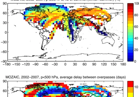
Figure 1 highlights this fact for upper tropospheric data (p_M<500 hPa, where p_M

stands for the flight altitude) over the period 2002–2007. The top figure shows the

10

fraction of measurements, in a 5◦×5◦ grid, taken in summer compared to the statis-tics including winter and summer for each latitude/longitude. The very large variability indicates that these data will sometimes include more statistics from winter measure-ments (over the Arctic for example) or from summer measuremeasure-ments (over Russia for example).

15

Moreover, statistics in each grid box are not sampled within regular time steps. To illustrate this, the bottom figure of Fig. 1 shows the average interval (in days) between overpasses for each grid box. Except on very common routes, such as the North-Atlantic Flight Corridor, overpasses are not obtained on a daily basis. Rather, about 5 days are necessary for further overpasses of a region, which is very sparse for accurate

20

statistics. 352 grid boxes have an average time step smaller than 10 days but 273 grid boxes have an average time step larger than 10 days, 67 grid boxes attain average delays larger than 100 days.

We derive relative humidity with respect to ice “RHi_M” as in Gierens et al. (1999) and only keep data of highest quality (tag “1”) with p_M<500 hPa and T <243 K so

25

(7)

ACPD

11, 12889–12947, 2011

N. Lamquin et al.

Title Page

Tables Figures

◭ ◮

Back Close

Full Screen / Esc

Discussion

P

a

per

|

Dis

cussion

P

a

per

|

Discussion

P

a

per

|

Discussio

n

P

a

per

|

stratosphere (higher values). We have collocated these data with the AIRS data to (1) investigate relationships between MOZAIC relative humidity and AIRS cloud properties and (2) to develop a calibration method for the detection of ice supersaturation within the AIRS data.

3 Synergy of AIRS and MOZAIC

5

3.1 AIRS-MOZAIC collocations and statistics

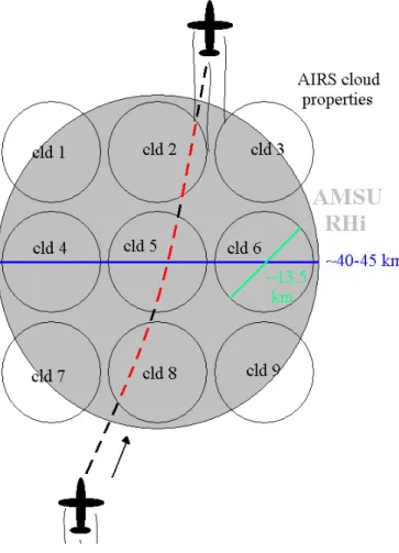
AIRS cloud properties are retrieved within each AIRS footprint of 13.5 km whereas RHi_Ais computed within the AMSU footprint of about 40 km. Therefore, we use two dif-ferent collocation schemes. When combining the AIRS cloud properties with MOZAIC RHi measurements we only keep the one flight measurement which is closest to the

10

center of the AIRS footprint and which is inside the AIRS footprint. When combining the AIRS relative humidity RHi_A with MOZAIC RHi we first collect all MOZAIC single measurements located within the AMSU footprint and then choose the highest relative humidity RHi_M among the collection of collocated measurements. In both cases data have to be coincident within a timeframe of 30 min.

15

The situation is illustrated in Fig. 2 where a MOZAIC flight is crossing an AMSU footprint. A maximum of about 50 collocated MOZAIC measurements (from one flight) can reside within one AMSU footprint. The high coverage and the large amount of AIRS data between 2003 and 2007 lead to a relatively large set of statistics. Table 2 shows statistics of collocated events (one MOZAIC single measurement per AIRS footprint)

20

in the upper troposphere (p <500 hPa) per latitude band and per AIRS scene divided into clear sky (“clear”), low and mid-level clouds (“lmclds”, p_cld>440 hPa) and high clouds (“cirrus”, p_cld<440 hPa). In brackets we indicate the fraction of all MOZAIC-AIRS collocations with respect to the total number of events per latitude band and with respect to the total number of collocations. A large majority of the collocations are

25

(8)

ACPD

11, 12889–12947, 2011

N. Lamquin et al.

Title Page

Tables Figures

◭ ◮

Back Close

Full Screen / Esc

Discussion

P

a

per

|

Dis

cussion

P

a

per

|

Discussion

P

a

per

|

Discussio

n

P

a

per

|

In the presence of cirrus clouds, keeping MOZAIC measurements close to the cirrus altitude (|p_M−p_cld|<50 hPa because of the cloud top uncertainty of AIRS) leads to a considerable reduction of the global cirrus statistics: 30% of the statistics are kept. The fraction of the total number of collocations representing measurements inside cirrus then decreases from 25% to about 8%. This is in agreement with Spichtinger et al.

5

(2004) who find between 2 and 8% at latitudes higher than 30◦ and between 13 and 33% at latitudes lower than 30◦ based on fits of the distributions of relative humidity from the MOZAIC data.

3.2 Relationships between MOZAIC relative humidity and AIRS-LMD cloud

properties

10

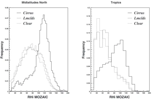
Figure 3 shows distributions of RHi_M, separately for three scene types: cirrus, clear sky and clouds with cloud-top pressure larger than 440 hPa (low and mid-level clouds). We compare two latitude bands: northern midlatitudes 40–60◦(left) and tropics 20◦N– 20◦S (right). For clear and lmclds situations RHi_Mcorresponds to measurements within the 200–250 and 250–300 hPa layers. In the case of cirrus, RHi_Mis measured close to

15

the cloud pressure with|p_M−p_cld|<50 hPa so that the distributions begin to represent what might actually be observed inside a cirrus layer. For every situation data are only considered below the tropopause. This is ensured by the MOZAIC criterion m_O₃<

130 ppbv and by the tropopause altitude provided in the AIRS L2 data.

In both latitude bands the distributions for clear skies are similar to those for low and

20

middle clouds. We observe drier upper tropospheric air in the tropics at aircraft cruise altitudes (mainly about 200–250 hPa), consistent with Fig. 4 of Gierens et al. (1999). For situations involving cirrus clouds we observe a peak frequency at 115–120% for the northern midlatitudes and around 100% for the tropics. In the tropics, the cruise altitude of aircraft does not coincide with the altitude where cirrus clouds are most commonly

25

(9)

ACPD

11, 12889–12947, 2011

N. Lamquin et al.

Title Page

Tables Figures

◭ ◮

Back Close

Full Screen / Esc

Discussion

P

a

per

|

Dis

cussion

P

a

per

|

Discussion

P

a

per

|

Discussio

n

P

a

per

|

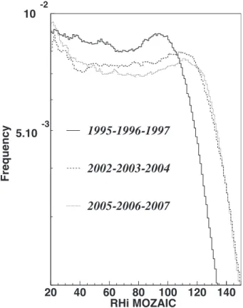
The peak value for the northern midlatitudes is wetter than expected from in situ measurements (Ovarlez et al., 2002; Immler et al., 2008). In fact, these authors show distributions of relative humidity inside cirrus clouds peaked around saturation. Our ob-servation of a peak higher than saturation agrees with the distributions of RHi_M (mea-sured in 2003) in Gettelman et al. (2006a) where RHi_M decreases more sharply after

5

120% but disagrees with distributions from Gierens et al. (1999) obtained from earlier MOZAIC data (1995–1997). Indeed, Gierens et al. (1999) show probability distributions of either tropospheric or stratospheric RHi_M. These distributions show a decrease be-yond 100% with a concomitant bulge highlighting the statistics of measurements inside cirrus clouds (Spichtinger et al., 2004). Figure 4 compares distributions of tropospheric

10

RHi_M (p <500 hPa, T <243 K andm_O₃<130 ppbv) obtained from MOZAIC-only data between 1995 and 1997 to distributions obtained from data between 2002 and 2004 and between 2005 and 2007. Compared to the years 1995 to 1997 the distributions over the periods 2002–2004 and 2005–2007 show a strong bias of about 10%, likely due to a calibration problem.

15

In the following we consider the occurrence of ice supersaturation detected by MOZAIC. For this purpose we need to take the measurement bias (for the MOZAIC time period used here: 2002–2007) into account by shifting the detection threshold by 10%: MOZAIC detects ice supersaturation only when RHi_M>110%. This is all the more reliable since the shape of the decreasing slope after saturation is unchanged.

20

Also, as Gierens et al. (1999) suggest for values of RHi_Maround saturation, an uncer-tainty∆RHi_M=±10% is taken into account.

3.3 Impact of fixed flight altitudes

We have to keep in mind that MOZAIC measurements are taken at only one level, corresponding to the actual flight altitude. There is no information on the thickness of

25

supersaturated layers. Even if the MOZAIC measurement is below an assumed ISS threshold of 110%, there may exist a layer of ISS below or above flight altitude. This potentially underestimates the occurrence of ice supersaturation detected by MOZAIC within the AIRS pressure layers of about 2 km.

(10)

ACPD

11, 12889–12947, 2011

N. Lamquin et al.

Title Page

Tables Figures

◭ ◮

Back Close

Full Screen / Esc

Discussion

P

a

per

|

Dis

cussion

P

a

per

|

Discussion

P

a

per

|

Discussio

n

P

a

per

|

To compensate for this effect we must lower the relative humidity threshold for ice supersaturation detection in MOZAIC. On the other hand, lowering this threshold in-creases the probability of false-alarms, that is to say the amount of supersaturation detected when there is no supersaturation in reality.

A new threshold has therefore been determined by simulating the success to detect

5

supersaturation in a collection of radiosoundings from routine measurements at Lin-denberg, Germany. These radiosounding measurements are corrected in the upper troposphere (Leiterer et al., 2005) and detect ice supersaturation (Spichtinger et al., 2003a; Lamquin et al., 2009).

The principle is the one of the Peirce skill-score (Peirce, 1884). It has notably been

10

used (and widely explained) in R ¨adel and Shine (2007) for an evaluation of the abil-ity of radiosounding measurements to detect cold ice supersaturated regions nesting persistent contrails.

For each AIRS pressure layer with top pressure larger than or equal to 200 hPa (because of the altitude of the tropopause in Lindenberg) a Monte-Carlo simulation is

15

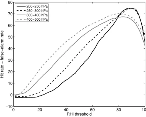
made over the collection of radiosonde profiles: it simulates for each profile a random altitude and, thus, a random measurement of relative humidity inside a pressure layer. An evaluation of the success to detect ice supersaturation by applying a threshold of relative humidity lower than saturation is made using the Peirce skill-score. It is simulated for each relative humidity threshold between 0 and 100%.

20

Figure 5 shows the skill-scores obtained for each of the four AIRS pressure layers between 200 and 500 hPa. For the pressure layers 200–250 and 250–300 hPa the score is maximum for a relative humidity threshold of about 90%. The distributions for the pressure layers 300–400 and 400–500 hPa are slightly broader with a peak around 85%. The difference is linked to the slightly larger vertical extension of these layers.

25

(11)

ACPD

11, 12889–12947, 2011

N. Lamquin et al.

Title Page

Tables Figures

◭ ◮

Back Close

Full Screen / Esc

Discussion

P

a

per

|

Dis

cussion

P

a

per

|

Discussion

P

a

per

|

Discussio

n

P

a

per

|

the detection of ice supersaturation within the boundaries of the AIRS pressure layers. To conclude, we consider ISS to be detected by MOZAIC at some location of a pres-sure layer when RHi_M>100±10%. Although this threshold would have naturally been used, only an understanding of the relationships presented above leads to its correct interpretation.

5

3.4 A calibration method for the determination of ice supersaturation

occurrence within AIRS pressure layers

The principle of the method was introduced in Lamquin et al. (2009). It is based on the determination of an occurrence probability of ISS as a function of coarse relative hu-midity measurements integrated over pressure layers. This occurrence probability can

10

either be the probability of “at least once” supersaturation (supersaturation exists some-where within the layer) or the probability of supersaturation weighted by the thickness of the supersaturated fraction of the layer (the weight being one if supersaturation cov-ers the whole pressure layer). The first approach is equivalent to the second approach when using a weight of one, whether the supersaturated layer is thin or thick.

Accord-15

ing to Spichtinger et al. (2003a) and R ¨adel and Shine (2007) ice supersaturated layers are indeed on average thinner (about 500–700 m) than the vertical spacing of the AIRS pressure layers (about 2 km). In Lamquin et al. (2009) the “at least once” approach was proposed because no accurate information on the thickness of supersaturated layers could be given. Dickson et al. (2010) investigated the weighted approach by using a

20

very large set of radiosonde measurements, they show that the so-called “S-function” depends mostly on the vertical resolution of the coarsely-determined relative humidity. As MOZAIC measurements do not allow the determination of the thickness of ice supersaturated layers, we must use the “at least once” approach and make a sensitivity analysis. The “at least once” statistics lead to higher ISS occurrences than the statistics

25

weighted by the thickness of the supersaturated layers (Figs. 3 and 4 of R ¨adel and Shine, 2007). This is important to keep in mind when comparisons are presented in Sect. 5 as we will compute ISS occurrence frequencies in other datasets in a similar way over pressure layers of finite depth.

(12)

ACPD

11, 12889–12947, 2011

N. Lamquin et al.

Title Page

Tables Figures

◭ ◮

Back Close

Full Screen / Esc

Discussion

P

a

per

|

Dis

cussion

P

a

per

|

Discussion

P

a

per

|

Discussio

n

P

a

per

|

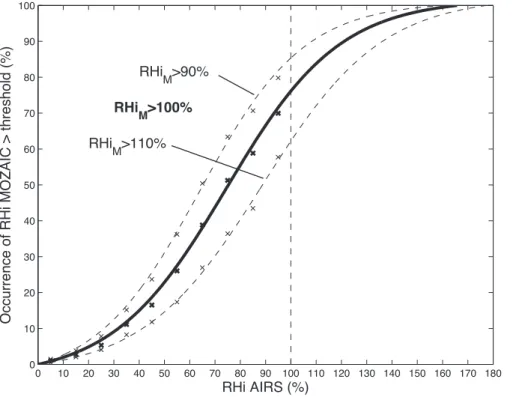
We now build the “S-function” by examining the probability of ice supersaturation computed from MOZAIC data collocated with AIRS relative humidity RHi_A. We reject AIRS bad quality data as well as RHi_A computed in pressure layers inside of which a tropopause is observed. Figure 6 then relates RHi_A and S_Th(RHi_A), the occurrence probability of ice supersaturation determined by the condition RHi_M>Th% with

ei-5

ther Th=90%, Th=100% or Th=110% to take into account the 10% uncertainty of MOZAIC.

The statistics drop progressively as RHi_A increases, without enough statistics at RHi_A>100% (less than 100 events per interval). Only statistically significant pairs (RHi_A, S_Th(RHi_A)) are shown, and each curve is fitted with a hyperbolic tangent for

10

further use.

Two conclusions can be drawn: first, we see that, even for Th=110%, a significant probability of ice supersaturation is found when RHi_Ais smaller than 100%. This is what we expected, as Kahn et al. (2008) and Lamquin et al. (2008) have already shown that very shallow ice clouds are concomitant with low RHi_A, highlighting the impact of the

15

coarse vertical resolution of the sounder.

Second, the occurrence of ice supersaturation reaches only about 85% for RHi_A val-ues around saturation even for Th₌90%. It can be argued that MOZAIC does not always locate ISS lying within the pressure layer even though we statistically com-pensate the e_ffect of having fixed flight altitudes in the timeframe of the collocation.

20

However, when RHi_A≈100% a substantial part of the pressure layer must be very humid thus decreasing the probability that MOZAIC misses ISS. Another explanation considers non-linear e_ffects of the AIRS vertical resolution on RHi_A. Unfortunately it is not possible to investigate it further as we do not have information on relative humidity profiles with MOZAIC.

25

(13)

ACPD

11, 12889–12947, 2011

N. Lamquin et al.

Title Page

Tables Figures

◭ ◮

Back Close

Full Screen / Esc

Discussion

P

a

per

|

Dis

cussion

P

a

per

|

Discussion

P

a

per

|

Discussio

n

P

a

per

|

saturation are shown because higher values do not provide enough statistics. In Fig. 7 occurrence probabilities of ice supersaturation are determined with Th=100%. The regional and seasonal variabilities are rather small compared to variabilities obtained for different temperature ranges or cloud scenes.

The interpretation of the differences observed for different cloud scenes is quite

5

straightforward. We distinguish between clear and cloudy situations in the upper tro-posphere: “clear” meaning “no clouds in the upper troposphere”, that is to say either clear sky or low and mid-level clouds. Using the retrieved emissivity we further separate cirrus situations into “thin cirrus” (ǫ_cld<0.5) and “cirrus” (ǫ_cld>0.5). Clearly, the occur-rence probability of ice supersaturation S(RHi_A) is increasing with cloudiness in the

10

upper troposphere. This highlights the effect of fixed flight altitudes of MOZAIC within the AIRS pressure layers. With increasing cloudiness portions of the atmospheric pro-files with high relative humidity are extending vertically, thus increasing the probability for MOZAIC aircraft to fly through supersaturated areas (either inside or in the vicinity of clouds). On average, the impact of fixed flight altitudes has been taken into account

15

by lowering the MOZAIC detection threshold Th. It could be considered relevant to use different S-functions depending on the cloud scene but we are interested in the occurrence of ice supersaturation within a pressure layer, independently of its vertical extent. The differences in Fig. 7 for different cloud scenes should not be considered as a bias in the present analysis.

20

For di_fferent temperature ranges there is no clear distinction between results ob-tained for the temperature ranges 220< T <230 K and T >230 K (with still T <243 K). However, Fig. 7 exhibits higher occurrence probability of ice supersaturation for the coldest temperatures (T <220 K). Gierens et al. (1999) show that ice supersaturated regions are, on average, colder than other regions in the upper troposphere. By

select-25

ing the coldest temperatures we might in turn get higher ice supersaturation occurrence probability simply by having a greater chance that MOZAIC meets supersaturation. Possible non-linear e_ffects of the AIRS vertical resolution on RHi_A might influence this comparison as temperature can vary as much as 5 to 10 K between the edges of the

(14)

ACPD

11, 12889–12947, 2011

N. Lamquin et al.

Title Page

Tables Figures

◭ ◮

Back Close

Full Screen / Esc

Discussion

P

a

per

|

Dis

cussion

P

a

per

|

Discussion

P

a

per

|

Discussio

n

P

a

per

|

pressure layers and MOZAIC can fly anywhere inside the layer. We can therefore only relate the observed di_fferences to global uncertainties. Again, we cannot investigate this any further as MOZAIC does not provide information on the vertical distribution of temperature and humidity.

Overall the S-function appears quite stable with di_fferences remaining within the

un-5

certainties arising from MOZAIC and its coupling with AIRS. The global uncertainty on this method is set by the two bracketing S-functionsS₉₀(RHi_A) andS₁₁₀(RHi_A).

3.5 Horizontal extent of ice supersaturated areas

The horizontal extent of ice supersaturated layers is a key feature for a large-scale model’s parameterization of ice supersaturation. Ice supersaturation can be detected

10

from each AIRS observation only in a probabilistic way. In fact the S-function only gives the probabilityS(RHi_A) that an observation contains ice supersaturation. To evaluate the horizontal extent of ice supersaturated areas, we link neighbouring observations satisfying the same condition on this probability: S(RHi_A)> α. To do so we built a simple clustering algorithm which groups AIRS observations belonging to the same

15

orbits and satisfying such condition with eitherα=40%, α=60%, orα=80%. Each observation is assigned the size of a square, the side of which is the diameter of the AMSU footprint and we take into account the variability of this size with the angle of observation. Clusters are constructed by grouping neighbouring observations of the same orbits and we do not relate adjacent orbits, therefore the clusters are limited by

20

the size of the AIRS swath (1650 km). The results possibly underestimate the true size of the clusters but the figures suggest that only very few clusters are extremely large.

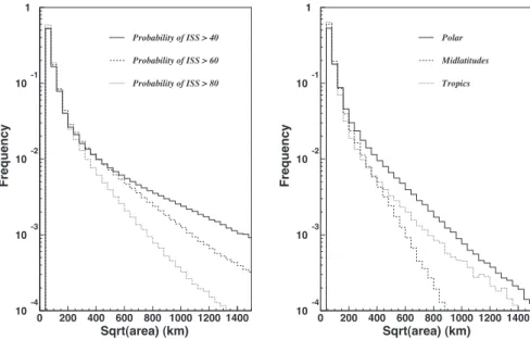
Figure 8 shows the distributions of the characteristic size (square root of the total area) of the clusters for (left) the three values of α for all regions combined and for (right)α=80% for three latitude bands: polar, (>70◦), midlatitudes (40◦–60◦N and S)

25

(15)

ACPD

11, 12889–12947, 2011

N. Lamquin et al.

Title Page

Tables Figures

◭ ◮

Back Close

Full Screen / Esc

Discussion

P

a

per

|

Dis

cussion

P

a

per

|

Discussion

P

a

per

|

Discussio

n

P

a

per

|

frequencies, than in the midlatitudes (see below Fig. 10). Overall, the large majority of characteristic sizes are smaller than 200 km which agrees qualitatively with Gierens and Spichtinger (2000).

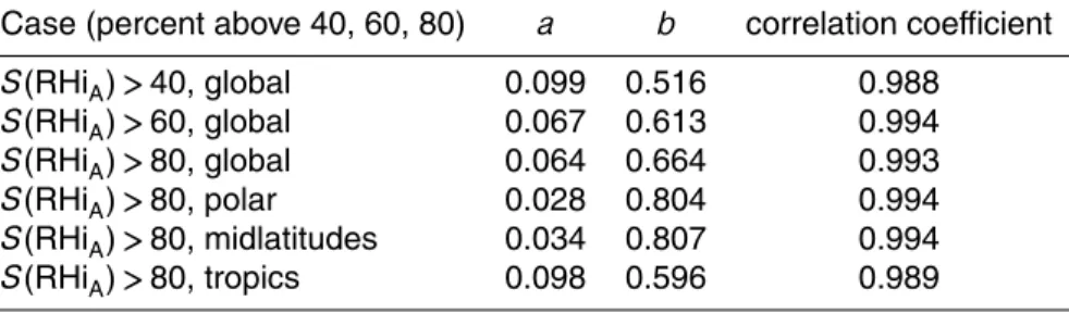
These distributions can be fitted by Weibull distributions (Gierens and Brinkop, 2002), i.e. functions of the form abxb−1e−axb. Using their cumulative distribution

5

F(x)₌1−e−axb a linear relationship exists between loglog1/(1−F) and log(x) as loglog1/(1−F)₌log(a)₊loglog(e)₊blog(x) (log is here with base 10). The histograms in Fig. 8 are then easily fitted using this relationship and Table 3 shows the parameters a and b of the Weibull function associated with each of these histograms as well as the very good correlation coe_fficient between the fit and the original histogram.

10

4 Climatology of the occurrence of ice supersaturation from AIRS

4.1 Climatology of ice supersaturation from AIRS

We have built a climatology of ice supersaturation occurrence by usingS₁₀₀(RHi_A) as a weighting function over each value RHi_A determined from the AIRS observations. The uncertainties are estimated by usingS₉₀(RHi_A) andS₁₁₀(RHi_A). To avoid potential

15

mixed-phase situations we include a temperature conditionT which is either 0 or 1. T

is set to zero when the temperature at the bottom of the pressure layer is higher than 243 K.

ISS occurrence frequencies are computed at a spatial resolution of 1◦lat×1◦lon for each pressure layerpas

20

ISS_p₌ PN

i=1S100(RHiA)× T

N (1)

whereN is the number of profiles of good quality in the upper troposphere over 1◦×1◦. To estimate the e_ffect of a possible bias arising from this selection, Fig. 9 presents

(16)

ACPD

11, 12889–12947, 2011

N. Lamquin et al.

Title Page

Tables Figures

◭ ◮

Back Close

Full Screen / Esc

Discussion

P

a

per

|

Dis

cussion

P

a

per

|

Discussion

P

a

per

|

Discussio

n

P

a

per

|

the distributions of MOZAIC relative humidities RHi_M when these measurements are collocated with either good quality AIRS data or all AIRS data. The slightly wetter dis-tribution obtained for all situations indicates that ice supersaturation occurrence ISS_p may be slightly underestimated when only good quality AIRS profiles are used.

Figure 10 presents our 6-yr (2003–2008) climatology of ice supersaturation

occur-5

rence in the upper troposphere for six AIRS pressure layers between 100 and 500 hPa. We have averaged daytime and nightime observations. We recall that results for pres-sure layers 100–150 and 150–200 hPa are only indicative because of the AIRS lower reliability at such high altitudes.

Whereas the functionS(RHi_A) is obtained from tropospheric data only, it is also used

10

when the pressure layer is partly or entirely within the stratosphere. In these cases RHi_Ais an “average” between the moister part of the layer lying in the troposphere and the drier part lying in the stratosphere. RHi_Ais decreased compared to its tropospheric counterpart. However,S(RHi_A) is also decreased which represents the fact that ice su-persaturation occurrence probability within the entire pressure layer is decreased. We

15

assume that the S-functionS(RHi_A) smoothly captures the transition from tropospheric to stratospheric air and ISS_pdecreases accordingly as we progress upward.

In Fig. 10 ice supersaturation occurrence frequencies mainly follow the tropopause with high frequencies close to the tropical tropopause in the pressure layer 100– 150 hPa, local maxima in connection with the storm tracks and jet streams in the

mid-20

latitudes at 200–250 hPa, and then close to the Arctic tropopause (about 300 hPa). Although only indicative, the tropical maximum at 100–150 hPa agrees qualitatively with clear-sky ISS statistics from the Microwave Limb Sounder (MLS) in Spichtinger et al. (2003b) at 147 hPa with frequencies up to 50% over areas of deep convec-tion. The seasonal difference between winter and summer is presented in Fig. 11.

25

It shows higher supersaturation frequencies during boreal winter, which again agrees with Spichtinger et al. (2003b). It is induced by a stronger convection over this period.

(17)

ACPD

11, 12889–12947, 2011

N. Lamquin et al.

Title Page

Tables Figures

◭ ◮

Back Close

Full Screen / Esc

Discussion

P

a

per

|

Dis

cussion

P

a

per

|

Discussion

P

a

per

|

Discussio

n

P

a

per

|

strong seasonal cycle of ISS frequencies with a maximum during boreal winter (about 35% in some portions of the atmosphere in their Fig. 6), in agreement with our results. Figure 12 shows the zonal means of ISS occurrences for winter (black lines) and summer (red lines) separately usingS100(RHiA) (plain) and the uncertaintiesS90(RHiA)

and S₁₁₀(RHi_A) (dashed). As can be deduced from Fig. 6, the uncertainty is about

5

±20% of the frequency values (i.e. lower for smaller ISS occurrence frequencies). The highest ISS occurrence frequencies are found close to the tropopause in the tropics and in the polar regions with maxima of about 50%.

4.2 Evaluation with MOZAIC

Although the climatology from MOZAIC is not global, an evaluation of the AIRS

cli-10

matology can be made over areas covered by the MOZAIC flight paths (northern mid-latitudes mainly). We restrict the analysis to the period 2002–2007 common to both datasets.

To compute ISS occurrence with MOZAIC we follow Gierens et al. (2000) and collect MOZAIC data over 5◦ lat × 5◦ lon grid cells, separately in the three pressure layers

15

150–200, 200–250 and 250–300 hPa. For these layers the MOZAIC statistics are the most plentiful. Only grid cells with statistics of more than one hundred measurements are kept. Both tropospheric and stratospheric data are used. We remind that ice super-saturation occurrence from AIRS represents the occurrence of supersuper-saturation at any altitude within a pressure layer (“at least once” supersaturation occurrence).

There-20

fore, it is important to determine ISS occurrence frequencies for MOZAIC in a similar manner. We use the same relative humidity threshold for the detection of ice super-saturation in the MOZAIC data as the one used to construct the S-function, that is to say RHi_M>100%. We have lowered the relative humidity threshold to compensate for the fact that MOZAIC does not detect supersaturation at altitudes below or above flight

25

altitude and between the pressure layer boundaries (see Sect. 3.3). The ISS frequen-cies from MOZAIC are then slightly higher in our calculation than the one in Gierens et al. (2000). As Fig. 4 supports, it can be shown that the statistics using RHi_M>110%

(18)

ACPD

11, 12889–12947, 2011

N. Lamquin et al.

Title Page

Tables Figures

◭ ◮

Back Close

Full Screen / Esc

Discussion

P

a

per

|

Dis

cussion

P

a

per

|

Discussion

P

a

per

|

Discussio

n

P

a

per

|

over the period 2002–2007 are comparable to the statistics using RHi_M>100% over the period 1995–1997.

Figure 13 presents maps of ISS occurrences from AIRS (left) and MOZAIC (right) for the years 2002–2007 and separately for the pressure layers 150–200, 200–250, and 250–300 hPa. For an easier comparison we mask the AIRS data corresponding

5

to grid cells where MOZAIC data are available. Geographical patterns and magni-tudes agree fairly well considering the limitations of spatial and temporal sampling by MOZAIC (Fig. 1 and Sect. 2.2). The differences are particularly apparent close to the tropopause and in regions with high seasonal variability (the Arctic for example) and/or small MOZAIC coverage. The AIRS climatology is less noisy than MOZAIC because

10

all seasons are equally well represented.

This comparison highlights the benefit of our method exploiting the synergy between AIRS and MOZAIC. We keep the best from these two datasets: the ability to detect thin supersaturated layers from MOZAIC and the global coverage from AIRS.

4.3 Relationship with cirrus cloud occurrences from CALIOP

15

CALIOP (Winker et al., 2003) is the first spaceborne lidar set for a long duration mis-sion. Its ability to determine accurate vertical profiles of clouds has been shown in the literature since its launch in 2006 (e.g. Winker et al., 2007, 2009; Mace et al., 2009; Stubenrauch et al., 2010). We recall that the analysis of a backscattered laser beam allows a vertical profiling of clouds having low optical depths (maximum about 5) with

20

vertical resolution of about 60 m in the upper troposphere. This instrument is therefore especially efficient for the detection of cirrus clouds.

To relate ice supersaturation occurrence from AIRS to high cloud occurrence from CALIOP we determine if clouds occupy one or several AIRS pressure layers. Since ice supersaturation may occur at any location inside the pressure layers, we state that a

25

(19)

ACPD

11, 12889–12947, 2011

N. Lamquin et al.

Title Page

Tables Figures

◭ ◮

Back Close

Full Screen / Esc

Discussion

P

a

per

|

Dis

cussion

P

a

per

|

Discussion

P

a

per

|

Discussio

n

P

a

per

|

one of the uppermost cloud layer) when retrieved by infrared sounders (Stubenrauch et al., 1999, 2010).

Cirrus occurrence per pressure layer is then determined from two years (2007–2008) of CALIOP data. Unfortunately the lidar nadir geometry prohibits reaching very high latitudes and statistics are therefore limited to latitudes between 80◦N and S. Figure 14

5

shows zonal means of ice supersaturation occurrence from AIRS data between 2007 and 2008 along with zonal means of cirrus occurrence, separately for the six pressure layers between 100 and 500 hPa.

The high cloud occurrence follows the ice supersaturation occurrence. This indicates the cause-to-consequence relationship between ice supersaturation and cirrus clouds:

10

ice clouds form where ice supersaturation takes place as the latter is a prerequisite for ice cloud formation.

In Gierens et al. (2000) correlations are shown between ice supersaturation oc-currence from MOZAIC and ococ-currence of subvisible cirrus detected from the Strato-spheric Aerosol and Gas Experiment (SAGE II Wang et al., 1996). Figure 15 extends

15

these relationships to all types of cirrus clouds with optical depth lower than about 5. The results are shown for the pressure layers below the tropopause in the tropics (0◦– 30◦N and S separately), in the midlatitudes (30◦–60◦N and S separately) and in the polar regions (60◦–90◦N and S separately). Cirrus occurrence statistics and ice super-saturation statistics are determined for each season at a spatial resolution of 1◦lat×1◦

20

lon, only statistics with more than one hundred CALIOP measurements are used. The standard deviation in Fig. 15 represents both the seasonal variability and the spatial variability of the relationship between cirrus and ice supersaturation occurrences. In addition, the sparse sampling of CALIOP (about one orbit every 1000 km and no swath) compared to AIRS may lead to sampling noise for cirrus occurrence.

25

The positive correlations suggest again the cause-to-consequence relationship be-tween ice supersaturation and cirrus clouds although the slopes of these correlations seem to decrease from about 1 in the tropics to about 0.5 in the polar regions. This could be linked to different lifetime and formation mechanisms of cirrus clouds.

(20)

ACPD

11, 12889–12947, 2011

N. Lamquin et al.

Title Page

Tables Figures

◭ ◮

Back Close

Full Screen / Esc

Discussion

P

a

per

|

Dis

cussion

P

a

per

|

Discussion

P

a

per

|

Discussio

n

P

a

per

|

Although only indicative in the tropics (AIRS reliability is lower at altitudes higher than 200 hPa), the absolute di_fference between the layer 100–150 hPa and the other layers may be explained by higher ISS occurrence frequencies (Fig. 10) close to the tropical tropopause. The standard deviation is larger in the pressure layer 100–150 hPa than in the lower layers because ice supersaturation occurrence from AIRS is much higher

5

during boreal winter than during boreal summer (Fig. 11) whereas cirrus cloud statistics from CALIOP do not follow such a strong variability (e.g. Nazaryan et al., 2008).

5 Comparisons with ice supersaturation occurrences from ECMWF and ECHAM

Ice supersaturation is still not represented in most global circulation models. The Inte-grated Forecast System (IFS) of the ECMWF (Tompkins et al., 2007) resolves

super-10

saturation whereas the ECHAM4 climate model infers supersaturation from the cloud scheme (Burkhardt et al., 2008). Evaluations of ISS statistics with observations are required for potential improvements of ISS parametrizations (e.g. Lamquin et al., 2008; R ¨adel and Shine, 2010). In the following we compare global AIRS ISS occurrence fre-quencies to those derived from two different models: the ECMWF forecast model and

15

the ECHAM4 climate model. The statistics from both models are calculated using the same temperature criterion as described in Sect. 4.1.

5.1 Comparison with ECMWF

Although AIRS radiances are assimilated in the ECMWF model (McNally et al., 2006) ice supersaturation, as derived from AIRS in this study, cannot be directly assimilated.

20

(21)

ACPD

11, 12889–12947, 2011

N. Lamquin et al.

Title Page

Tables Figures

◭ ◮

Back Close

Full Screen / Esc

Discussion

P

a

per

|

Dis

cussion

P

a

per

|

Discussion

P

a

per

|

Discussio

n

P

a

per

|

For this purpose, high vertical resolution forecasts are extracted globally for the whole year 2007. They consist of 24 h-forecasts of relative humidity and temperature simulated at a spectral resolution of T799 (about 25 km at the equator) and 91 layers in the vertical (about 15 hPa). 24 h-forecasts are used rather than initial fields at 0-h lead time because of the spinup behaviour of ice supersaturation in the IFS (Lamquin et al.,

5

2009).

We extracted data in a regular 0.5◦×0.5◦ grid with vertical levels spaced by 25 hPa between 100 and 500 hPa. For the comparison the ice supersaturation occurrence frequencies in the IFS are computed using a “layer supersaturation” scheme declaring ice supersaturation present within one pressure layer (e.g. 200–250 hPa) when any

10

of the vertical levels of this layer exhibits ice supersaturation (in this case: 200, 225 or 250 hPa). For comparison we also show zonal means obtained from ISS statistics by only considering the single level lying in the middle of the layers (here that would be 225 hPa). Consequently, the former frequencies are always higher than the latter except near the subtropics in the layers 300–400 and 400–500 hPa because of the

15

temperature criterion (T always lower than 243 K). This criterion is applied to the bottom level for the “layer supersaturation” scheme whereas it is applied to the middle level in the other scheme, at relatively low altitudes this criterion may be fulfilled for the middle level but not for the bottom level resulting in higher occurrences of supersaturation with the middle level scheme.

20

Figures 16 and 17 first present climatologies of ISS occurrence frequencies from the IFS and its difference between boreal winter and summer for the year 2007. Even though the AIRS climatology covers 6 yr (only one year of data has been extracted from the IFS) Figs. 16 and 17 show a good correspondence with the geographical patterns and magnitudes seen in Figs. 10 and 11. However, for the IFS, Fig. 16 shows slightly

25

higher frequencies in the tropics and in the regions of the storm tracks and jet streams. For the year 2007 Fig. 18 shows the zonal means of ISS occurrence frequencies from AIRS (plain black) as well as its uncertainties (dashed black). In red, zonal means from the IFS are shown (solid line) with the dashed line indicating ISS at the middle

(22)

ACPD

11, 12889–12947, 2011

N. Lamquin et al.

Title Page

Tables Figures

◭ ◮

Back Close

Full Screen / Esc

Discussion

P

a

per

|

Dis

cussion

P

a

per

|

Discussion

P

a

per

|

Discussio

n

P

a

per

|

level of the layer. In this figure the zonal means from the IFS remain within or close to the uncertainties of our AIRS climatology. However the IFS has larger ISS occurrences in the tropics above 200 hPa, around the position of the tropopause break between 150 and 250 hPa between latitudes 40◦and 60◦(N and S), and in the Arctic in the pressure layer 200–250 hPa.

5

In the IFS, close to the tropical tropopause, ice supersaturation is taking place on a thin vertical scale around 100 hPa (see Tompkins et al., 2007). If such a model is realistic, then it is possible that AIRS agrees more with the “middle layer” ISS (here at 150 hPa) because the S-function does not capture the strong gradient of relative humidity between 100 and 150 hPa. Also, the S-function is not specifically designed

10

for levels 100–150 and 150–200 hPa because AIRS-MOZAIC collocations are too few at such altitudes in the tropics. We also remind that we must remain cautious with the AIRS water vapour data at this altitude (Fetzer et al., 2008). The disagreements around the tropopause break and in the Arctic suggest that the ISS layer estimate (i.e. using the “layer supersaturation” scheme) more abruptly captures the transition

15

between tropospheric and stratospheric air as supersaturation may be present at the bottom of the layer while the upper parts of it are in the stratosphere. The ECMWF ISS occurrences seem to have a stronger increase with altitude than the AIRS occurrences, which can be another side-effect of the “layer supersaturation” scheme because of the strong variability of the saturation specific humidity with temperature.

20

Figure 19 shows the zonal di_fferences between boreal winter and boreal summer. The uncertainties for AIRS are determined by the sum ∆ of the uncertainties from the summer and winter climatologies ((S90(RHiA)−S110(RHiA))/2 for each season).

Again, the ECMWF ISS layer estimate lies within the uncertainties (S₁₀₀(RHi_A)_{+ ∆}and

S₁₀₀(RHi_A)−∆) except near the tropical tropopause where the movement of the

Inter-25

(23)

ACPD

11, 12889–12947, 2011

N. Lamquin et al.

Title Page

Tables Figures

◭ ◮

Back Close

Full Screen / Esc

Discussion

P

a

per

|

Dis

cussion

P

a

per

|

Discussion

P

a

per

|

Discussio

n

P

a

per

|

5.2 Comparison with ECHAM

In the ECHAM4 climate model (R ¨ockner et al., 1996) ice supersaturation frequency has been parameterized consistent with the cloud scheme (Burkhardt et al., 2008) in order to enable the simulation of the climate effect of contrail cirrus (Burkhardt et al., 2009). The parameterization uses the information on subgrid scale variability of relative

5

humidity that is inherent in the parameterization of fractional cloud coverage and infers a fractional supersaturated area. The model has been run with a T30/L39 resolution for 5 yr and we compare the resulting climatology with observations. Vertical levels were spaced between 100 hPa and 200 hPa by 15 hPa and the spacing increased slowly to 30 hPa between 400 hPa and 500 hPa.

10

Due to the coarse horizontal resolution of the model we calculate the fractional su-persaturated area at each level within a pressure layer. We then apply a maximum random overlap scheme (as used in the cloud scheme) in order to calculate the frac-tional supersaturated area for a specified layer.

Ice supersaturation occurrence is then assessed globally in the same pressure layers

15

100–150 hPa, 150–200 hPa, 200–250 hPa, 250–300 hPa, 300–400 hPa, 400–500 hPa at the ECHAM spatial resolution of 3.75◦ lat ×3.75◦ lon. Figures 20 and 21 show respectively the global occurrences of ice supersaturation over the 5 yr of simulation and the difference between boreal winter and summer. We recall that results for pres-sure layers 100–150 and 150–200 hPa are less reliable due to the AIRS sensitivity and

20

therefore only indicative.

Despite the low resolution of the climate model the geographical patterns and abso-lute values of supersaturation are quite well represented. The most obvious deficiency is that in the 150–200 hPa and the 200–250 hPa layers the climate model overestimates supersaturation frequency in the extratropics. This is due to the fact that the model’s

25

tropopause is too high in the extratropics so that those layers are too frequently part of the troposphere. The bias in tropopause height is connected with the model’s lower stratospheric cold bias, a common problem in climate models (particularly at low reso-lution).

(24)

ACPD

11, 12889–12947, 2011

N. Lamquin et al.

Title Page

Tables Figures

◭ ◮

Back Close

Full Screen / Esc

Discussion

P

a

per

|

Dis

cussion

P

a

per

|

Discussion

P

a

per

|

Discussio

n

P

a

per

|

Therefore, we compare ECHAM zonal mean fractional supersaturated areas with troposphere only supersaturation frequencies from AIRS. The latter is computed using only tropospheric data (we reject data when the tropopause is lying inside the pres-sure layer). For comparison we also show the total (tropospheric and stratospheric) AIRS occurrences as they are computed for Fig. 18 (only computed usingS₁₀₀(RHi_A)).

5

Additionally, ISS occurrences from AIRS have been degraded to the ECHAM spatial resolution. When ISS is computed only over tropospheric data, very few observations are taken into account for pressure layers close to the tropopause. As a consequence, pressure layers between 100 and 250 hPa can only be computed by combining all sea-sons as there are not enough data available separately for each season.

10

Figure 22 shows zonal means of AIRS (plain and dashed black as in Fig. 18 but for tropospheric data only, plain gray for tropospheric plus stratospheric data) and ECHAM ISS occurrence frequencies (plain red). Figure 23 shows the winter minus summer dif-ference as in Fig. 19. In the tropics the ECHAM supersaturation frequencies are close to the AIRS supersaturation estimates at all levels. At lower layers ISS is mostly well

15

reproduced except at latitudes poleward of 60◦(N and S) where ISS is underestimated by ECHAM.

ECHAM4 is unable to reproduce the rise in ISS at 40◦S that is connected with the southern hemispheric storm track. At the upper layers the comparison is difficult since the tropospheric only estimates of AIRS consist only of very few data. Nevertheless,

20

ECHAM supersaturation remains mostly in between AIRS ISS and the AIRS tropo-spheric only ISS estimates. An exception are the midlatitudes at the 150–200 hPa layer, an area in which the IFS estimates are slightly too high as well and the AIRS data less reliable. In Fig. 23 the seasonal variations follow these observations. ECHAM shows a smaller variability of the difference between winter and summer ISS occurrences as a

25

(25)

ACPD

11, 12889–12947, 2011

N. Lamquin et al.

Title Page

Tables Figures

◭ ◮

Back Close

Full Screen / Esc

Discussion

P

a

per

|

Dis

cussion

P

a

per

|

Discussion

P

a

per

|

Discussio

n

P

a

per

|

6 Conclusions

We have presented a climatology of ice supersaturation occurrence from AIRS obser-vations covering the period 2003–2008. The relatively coarse vertical resolution of the AIRS retrieved water vapour profiles prohibits the direct detection of shallow supersat-urated layers. Therefore, we have developed a calibration method for the detection

5

of ice supersaturation by AIRS: space and time collocations of the detection of ice supersaturation by MOZAIC with coarsely-determined relative humidity profiles from AIRS allows the determination of an a priori probability function (the “S-function”) of ice supersaturation occurrence for any relative humidity value determined by AIRS. The horizontal extent of ice supersaturation is an important feature for large-scale model

10

parameterization, an evaluation of it is presented by use of a simple cluster analysis and its distribution can easily be fitted by a Weibull distribution.

We have used the S-function to establish a climatology of ice supersaturation occur-rence over the whole upper troposphere. However, due to the lower reliability of AIRS data at high altitudes, results in pressure layers 100–150 and 150–200 hPa are only

15

indicative. These statistics represent the probability that ice supersaturation occurs at least once within a given pressure layer. It compares relatively well to other pre-existant climatologies with high supersaturation occurrences near the tropical tropopause, in the region of the storm tracks and jet streams in the midlatitudes and close to the Arctic tropopause with a concomitant seasonal cycle. An evaluation of the

climatol-20

ogy is presented with statistics from MOZAIC only; it shows the benefit obtained from the synergy between AIRS and MOZAIC. A correlation with cirrus cloud statistics from CALIOP shows the cause-to-consequence link between ice supersaturation and cirrus cloud formation: cirrus clouds form where ice supersaturation takes place.

Finally, we compare the AIRS climatology to model climatologies from ECMWF

25

24 h-forecasts and ECHAM4 between 100 and 500 hPa. Except close to the tropical tropopause and in regions with possible influence of the tropopause lying within pres-sure layers, the comparison with the ECMWF forecasts is good. The climatology from

(26)

ACPD

11, 12889–12947, 2011

N. Lamquin et al.

Title Page

Tables Figures

◭ ◮

Back Close

Full Screen / Esc

Discussion

P

a

per

|

Dis

cussion

P

a

per

|

Discussion

P

a

per

|

Discussio

n

P

a

per

|

ECHAM4 has a lower horizontal resolution and therefore exhibits a smaller variability than AIRS and ECMWF. Nevertheless, it captures the main patterns of ISS success-fully in the upper troposphere. ECHAM exhibits a smaller meridional gradient than the observations and the ECMWF model at levels below 250 hPa.

Overall, this paper presents a way of dealing with the di_fficulty of remotely sensing

5

ice supersaturation and comparing statistics from various observations and models. We propose a bridge between those different means of investigation by the use of the synergy between infrared sounding and in situ measurements. Among future appli-cations of this work a climatology of potential condensation trails from aircraft will be assessed.

10

Acknowledgements. This work was supported by CNRS and Ecole Polytechnique. The AIRS version 5 data were obtained through the Goddard Earth Sciences Data and Information Ser-vices (http://daac.gsfc.nasa.gov/) and the CALIOP data were obtained through the Atmospheric Sciences Data Center (ASDC) at NASA Langley Research Center by the ICARE Thematic Center created by CNES (http://www-icare.univ-lille1.fr/) and its interface ClimServ created for 15

Institut Pierre-Simon Laplace (http://climserv.ipsl.polytechnique.fr/). ECMWF data have been retrieved within the framework of a special project on “Ice Supersaturation and Cirrus Clouds (SPDEISSR)”. The authors thank all the corresponding teams for assistance and public release of data products. The work contributes to COST Action ES-0604 “Water Vapour in the Climate System (WaVaCS)” and to the aforementioned SPDEISSR.

20