AMTD
3, 3925–3969, 2010Aircraft-borne DOAS limb measurements
C. Prados-Roman et al.
Title Page
Abstract Introduction
Conclusions References
Tables Figures
◭ ◮
◭ ◮
Back Close
Full Screen / Esc
Printer-friendly Version Interactive Discussion
Discussion
P
a
per
|
Dis
cussion
P
a
per
|
Discussion
P
a
per
|
Discussio
n
P
a
per
|
Atmos. Meas. Tech. Discuss., 3, 3925–3969, 2010 www.atmos-meas-tech-discuss.net/3/3925/2010/ doi:10.5194/amtd-3-3925-2010
© Author(s) 2010. CC Attribution 3.0 License.
Atmospheric Measurement Techniques Discussions
This discussion paper is/has been under review for the journal Atmospheric Measure-ment Techniques (AMT). Please refer to the corresponding final paper in AMT
if available.
Airborne DOAS limb measurements of
tropospheric trace gas profiles: case
study on the profile retrieval of O
4
and
BrO
C. Prados-Roman1, A. Butz2, T. Deutschmann1, M. Dorf1, L. Kritten1, A. Minikin3, U. Platt1, H. Schlager3, H. Sihler1,4, N. Theys5, M. Van Roozendael5, T. Wagner4, and K. Pfeilsticker1
1
Institute of Environmental Physics, University of Heidelberg, Germany
2
Netherlands Institute for Space Research – SRON, Utrecht, The Netherlands
3
Institut f ¨ur Physik der Atmosph ¨are, Deutsches Zentrum f ¨ur Luft- und Raumfahrt (DLR), Oberpfaffenhofen, Germany
4
AMTD
3, 3925–3969, 2010Aircraft-borne DOAS limb measurements
C. Prados-Roman et al.
Title Page
Abstract Introduction
Conclusions References
Tables Figures
◭ ◮
◭ ◮
Back Close
Full Screen / Esc
Printer-friendly Version Interactive Discussion
Discussion
P
a
per
|
Dis
cussion
P
a
per
|
Discussion
P
a
per
|
Discussio
n
P
a
per
|
5
Belgian Institute for Space Aeronomy – BIRA-IASB, Belgium
AMTD
3, 3925–3969, 2010Aircraft-borne DOAS limb measurements
C. Prados-Roman et al.
Title Page
Abstract Introduction
Conclusions References
Tables Figures
◭ ◮
◭ ◮
Back Close
Full Screen / Esc
Printer-friendly Version Interactive Discussion
Discussion
P
a
per
|
Dis
cussion
P
a
per
|
Discussion
P
a
per
|
Discussio
n
P
a
per
|
Abstract
A novel limb scanning mini-DOAS spectrometer for the detection of UV/vis absorb-ing radicals (e.g., O3, BrO, IO, HONO) was deployed on the DLR-Falcon (Deutsches
Zentrum f ¨ur Luft- und Raumfahrt) aircraft and tested during the ASTAR 2007 cam-paign (Arctic Study of Tropospheric Aerosol, Clouds and Radiation) that took place at
5
Svalbard (78◦N) in spring 2007. Our main objectives during this campaign were to test the instrument, and to perform spectral and profile retrievals of tropospheric trace gases, with particular interest on investigating the distribution of halogen compounds (e.g., BrO) during the so-called ozone depletion events (ODEs). In the present work, a new method for the retrieval of vertical profiles of tropospheric trace gases from
tropo-10
spheric DOAS limb observations is presented. Major challenges arise from modeling the radiative transfer in an aerosol and cloud particle loaded atmosphere, and from overcoming the lack of a priori knowledge of the targeted trace gas vertical distribu-tion (e.g., unknown tropospheric BrO vertical distribudistribu-tion). Here, those challenges are tackled by a mathematical inversion of tropospheric trace gas profiles using a
regular-15
ization approach constrained by a retrieved vertical profile of the aerosols extinction coefficientEM. The validity and limitations of the algorithm are tested with in situ mea-sured EM, and with an absorber of known vertical profile (O4). The method is then
used for retrieving vertical profiles of tropospheric BrO. Results indicate that, for air-craft ascent/descent observations, the limit for the BrO detection is roughly 1.5 pptv
20
(pmol/mol), and the BrO profiles inferred from the boundary layer up to the upper tro-posphere and lower stratosphere have around 10 degrees of freedom.
For the ASTAR 2007 deployments during ODEs, the retrieved BrO vertical profiles consistently indicate high BrO mixing ratios (∼15 pptv) within the boundary layer, low BrO mixing ratios (≤1.5 pptv) in the free troposphere, occasionally enhanced BrO
mix-25
AMTD
3, 3925–3969, 2010Aircraft-borne DOAS limb measurements
C. Prados-Roman et al.
Title Page
Abstract Introduction
Conclusions References
Tables Figures
◭ ◮
◭ ◮
Back Close
Full Screen / Esc
Printer-friendly Version Interactive Discussion
Discussion
P
a
per
|
Dis
cussion
P
a
per
|
Discussion
P
a
per
|
Discussio
n
P
a
per
|
1 Introduction
The Differential Optical Absorption Spectroscopy (DOAS) is a well known and estab-lished atmospheric measurement technique (Platt and Stutz, 2008). In many applica-tions using scattered skylight, the main challenge of the remote sensing DOAS method lies in retrieving trace gas concentrations from the measured differential slant column
5
densities (dSCDs). Trace gas concentrations are inferred by consecutively probing the air masses at different viewing geometries, and a subsequent mathematical inversion of the whole set of observations (e.g., Rodgers, 2000). In the best case scenario, the sampling is arranged so that the amount of pieces of independent information on the multi-dimensional (spatial and temporal) distribution of the targeted species is
maxi-10
mized. In practice however, the degrees of freedom are often limited since the chang-ing viewchang-ing geometries are predetermined by movements of the light source (e.g., by celestial light sources), by displacements of the instrument platform (ships, aircrafts, balloons, satellites, etc), by the change of the viewing direction of the light receiving telescope, or by a combination of all of the above. Gathering the information often
re-15
quires sampling over a large spatial or temporal domain of the atmosphere, in which the radiative transfer (RT) may change considerably as well. The need of dealing with these observational limitations correctly, and of accounting for the atmospheric RT of each in-dividual measurement properly, defines a rather complicated (and in general ill-posed) mathematical inversion problem. As solutions largely depend on the individual kind of
20
observations, different strategies have been developed to solve these ill-posed inver-sion problems (e.g., Rodgers, 2000). This paper reports on aircraft-borne observations of important and rare trace gases (e.g., tropospheric BrO) monitored in a heteroge-neously scattering atmosphere (the Arctic spring troposphere). Herein, a dedicated method for the profile retrieval of trace gases constrained by means of measured
rela-25
Un-AMTD
3, 3925–3969, 2010Aircraft-borne DOAS limb measurements
C. Prados-Roman et al.
Title Page
Abstract Introduction
Conclusions References
Tables Figures
◭ ◮
◭ ◮
Back Close
Full Screen / Esc
Printer-friendly Version Interactive Discussion
Discussion
P
a
per
|
Dis
cussion
P
a
per
|
Discussion
P
a
per
|
Discussio
n
P
a
per
|
like Vlemmix et al. (2010), here not just the total aerosol optical thickness is inferred, but vertical profiles of the extinction coefficient (EM) of aerosol and cloud particles (from now on referred to as “aerosols”). The targeted trace gas profile inversion, constrained by the retrieved aerosolEM, is then addressed with a regularization approach using no
a priori knowledge of its vertical distribution (e.g., Phillips, 1962; Rodgers, 2000).
5
The validity of the novel algorithm is demonstrated for deployments of an optical spectrometer (a mini-DOAS instrument) on the DLR-Falcon aircraft during the ASTAR 2007 campaign. Within the framework of the International Polar Year 2007/08, and as part of the POLARCAT project (“Polar Study using Aircraft, Remote Sensing, Sur-face Measurements and Models, of Climate, Chemistry, Aerosols, and Transport”), the
10
ASTAR 2007 campaign aimed at investigations during the Arctic haze season (e.g., Quinn et al., 2007). The campaign was based on Spitsbergen (78◦N, 18◦E) and took place during March and April 2007. During this field campaign, target trace gases to be detected from the boundary layer (BL) up to the upper troposphere/lowermost strato-sphere (UT/LS) with the mini-DOAS instrument were O3, NO2, BrO, OClO, IO, OIO,
15
HONO, C2H2O2, CH2O, H2O and O4. Since recent studies point out the relevance of
halogens for the tropospheric photochemistry (e.g., von Glasow and Crutzen, 2003), this work primarily focuses on the detection and retrieval of bromine monoxide (BrO). Indeed, reactive halogen compounds (i.e., RHC=X, XO, X2, XY, OXO, HOX, XONO2,
XNO2, with X, Y as I, Br and Cl) are known to be key species, e.g., for the oxidation
20
capacity of the troposphere and for the lifetime limitation of other species such as O3,
HOx, NOxand dimethylsulfide. RHC are also known to be involved in new particle
for-mation (by iodine compounds, e.g., O’Dowd et al., 2002). Moreover, RHC are related to atmospheric mercury depletion events that eventually yield scavenge of Hg by snow and particles, and deposition of toxic mercury to the polar ecosystems (e.g., Steffen et
25
AMTD
3, 3925–3969, 2010Aircraft-borne DOAS limb measurements
C. Prados-Roman et al.
Title Page
Abstract Introduction
Conclusions References
Tables Figures
◭ ◮
◭ ◮
Back Close
Full Screen / Esc
Printer-friendly Version Interactive Discussion
Discussion
P
a
per
|
Dis
cussion
P
a
per
|
Discussion
P
a
per
|
Discussio
n
P
a
per
|
references therein). While the horizontal extent of the BrO associated with young sea ice is fairly well captured by total column satellite measurements (e.g., SCIAMACHY, GOME, OMI), a detailed tropospheric distribution profile of bromine monoxide mixing ratios remains uncertain. This lack of tropospheric BrO vertical profile climatology dur-ing the polar sprdur-ing is the trigger for the development of the retrieval method presented
5
herein.
The paper is structured in four main sections. In Sect. 2, all elements of the retrieval algorithm are introduced and described. This includes brief descriptions of (1) the mini-DOAS instrument, (2) the measurement technique and the spectral analysis, and (3) the applied inversion methods, i.e., the characterization of scattering events present
10
in the atmosphere via a non-linear inversion of the vertical profile of theEM, and the regularization of the targeted trace gas vertical profile. Section 3 addresses (1) the rigor of the assumptions needed for the RT modeling, (2) the validation and sensitivity of our method to retrieveEM vertical profiles, and (3) the robustness and sensitivity of the profile regularization of tropospheric trace gases, tested with the absorber of known
15
vertical distribution in the troposphere O4 (O2–O2collisional dimer, e.g., Pfeilsticker et
al., 2001). Section 4 presents the inferred BrO mixing ratio vertical profiles, compares them to other in situ measured trace gases (O3, CO) and to total BrO column densities
measured by satellite, and discusses the results. Finally, Sect. 5 summarizes and concludes the study.
20
2 Method
This section introduces the mini-DOAS instrument deployed during the ASTAR 2007 campaign, as well as the spectral measurement and analysis. Furthermore, the theory behind the retrieval algorithm (i.e, the nonlinear inversion of theEM vertical profile and
the regularization of the trace gas profile) is described.
AMTD
3, 3925–3969, 2010Aircraft-borne DOAS limb measurements
C. Prados-Roman et al.
Title Page
Abstract Introduction
Conclusions References
Tables Figures
◭ ◮
◭ ◮
Back Close
Full Screen / Esc
Printer-friendly Version Interactive Discussion
Discussion
P
a
per
|
Dis
cussion
P
a
per
|
Discussion
P
a
per
|
Discussio
n
P
a
per
|
2.1 Instrument
The present mini-DOAS instrument uses scattered sunlight received from the horizon for the detection of trace gases such us O3, NO2, BrO, OClO, IO, OIO, HONO, C2H2O2,
CH2O, H2O and O4. The technique has been developed by the Institute of Environ-mental Physics at the University of Heidelberg (IUP-HD), and validated via many
strato-5
spheric balloon flights during the past several years (e.g., Weidner et al., 2005; Kritten et al., 2010).
The novel mini-DOAS instrument deployed during the ASTAR 2007 campaign con-sists of a housing with two Ocean Optics spectrometers (QE65000/USB2000 for UV/vis) for the detection of skylight in the spectral range of 320–550 nm. In order
10
to assure optical stability, the spectrometers housing is evacuated, vacuum-sealed and temperature stabilized. The QE65000 and USB2000 spectrometers used have spectral resolutions (FWHM) of 0.4 nm (4.75 pixels) and 0.7 nm (6.2 pixels), respectively. The small size (483×400×270 mm3), weight (25 kg) and power consumption (14 W) make this mini-DOAS a versatile instrument for many measurement platforms. Indeed, since
15
the instrument was built in 2007, the specific instrument has been deployed on the Falcon aircraft, on balloon gondolas (MIPAS or LPMA/DOAS), and on manned (Geo-physica) and in future unmanned (Global Hawk) high-altitude aircrafts. In the case of the Falcon aircraft deployment, the two spectrometers, the stepper-motor controller, the computer and the display are integrated into a 19-inch rack inside of the
pressur-20
ized cabin. Two fiber bundles (for the UV/vis) directed the light from the two telescopes to the spectrometers. The two telescopes are mounted on two stepper-motors located in an aluminum air-tide window with two slits in the left side of the aircraft, exposed to the skylight with a field-of-view of 0.2◦ in the vertical. During the ASTAR 2007 cam-paign, both telescopes (for the UV/vis channels) were fixed parallel to the ground so
25
measure-AMTD
3, 3925–3969, 2010Aircraft-borne DOAS limb measurements
C. Prados-Roman et al.
Title Page
Abstract Introduction
Conclusions References
Tables Figures
◭ ◮
◭ ◮
Back Close
Full Screen / Esc
Printer-friendly Version Interactive Discussion
Discussion
P
a
per
|
Dis
cussion
P
a
per
|
Discussion
P
a
per
|
Discussio
n
P
a
per
|
ments collected by the UV channel, with a temporal resolution of∼10 s, depending on sampling conditions.
2.2 Measurement technique and spectral analysis
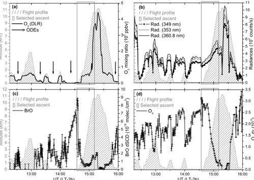
During the ASTAR 2007 campaign one sortie, performed on 8 April 2007, was specially devoted to probe the Arctic atmosphere for halogen activation (e.g., BrO detection) and
5
the development of ODEs over sea ice regions (see Fig. 1a). This work particularly
focuses on the O4, BrO and radiance measurements performed during a particular
aircraft ascent, marked by the box in Fig. 1. That particular ascent started at around 14:30 UT, while flying over sea ice at∼81◦N and 7◦E, with northwesterly ground winds of 6 m/s. During the approximately 30 min of the ascent, the aircraft climbed from
10
around 50 m of altitude up to 10.5 km, thus probing the Arctic atmosphere from the BL up to the UT/LS.
The DOAS method is applied for the spectral retrieval of O4and BrO (see Fig. 1c,d)
after all the spectra are corrected for electronic dark current and offset, and all the trace gas cross-sectionsσare convolved to the spectral resolution of our instrument. Using
15
the WinDOAS software (Fayt and Van Roozendael, 2001), the measured spectra are analyzed with respect to a spectrum measured when the aircraft entered the LS at around 15:10 UT (referred to asreferenceorFraunhofer spectrum in Platt and Stutz, 2008). As a result, the differential slant column densities (dSCDs) can be inferred.
The retrieval of the BrO dSCDs presented in Fig. 1c is based on the study of
Ali-20
well et al. (2002). Sensitivity studies performed with the temperature dependent BrO absorption cross-section (i.e., forT=298 K and 228 K) show non-negligible influence of the temperature on the retrieved BrO dSCDs in the BL. Indeed, within the BL, the BrO dSCDs retrieved considering the BrO cross-section at 228 K differ by ca. 20% from the BrO dSCDs retrieved using the BrO cross-section at 298 K. In order to take into
25
AMTD
3, 3925–3969, 2010Aircraft-borne DOAS limb measurements
C. Prados-Roman et al.
Title Page
Abstract Introduction
Conclusions References
Tables Figures
◭ ◮
◭ ◮
Back Close
Full Screen / Esc
Printer-friendly Version Interactive Discussion
Discussion
P
a
per
|
Dis
cussion
P
a
per
|
Discussion
P
a
per
|
Discussio
n
P
a
per
|
average of the BrO dSCDs retrieved at 228 K, and those retrieved at 298 K. Noteworthy is that this temperature dependency of the retrieved BrO dSCDs becomes impercepti-ble in the UT/LS since the BrO dSCDs retrieved at 228 K fall within the error margins of the BrO dSCD retrieved at 298 K.
The UV spectral retrieval of O4 is performed in the 346–366 nm wavelength
inter-5
val using the O4 cross-section of Hermans (2002). The interfering species i.e. O3 at
221 K (Burrows et al., 1999), NO2at 220 K (Van Daele et al., 1998) and BrO at 228 K (Wilmouth et al., 1999) are also included in the O4fitting procedure. Results are shown
in Fig. 1d. In this work the O4absorption is used for probing the characterization of the
light path in the forward RT model (see Sect. 3.2). In addition, O4 is also used for the
10
self-validation of our trace gas vertical profile retrieval (see Fig. 3.3). Since the vertical distribution of O4is related to the (squared) oxygen number density [O2], O4differential
optical densities (d τ=σ·dSCD) can be derived from the atmospheric temperature and pressure. The O4absorption cross-section is temperature dependent and its absolute value is not known up to date (Pfeilsticker et al., 2001). The O4 extinction coefficient
15
(EO4) presented in this work is calculated as
EO4=σ(T)·[O4]=σ·Keq(T)·[O2]2 (1)
whereKeq is the equilibrium constant of O4and, at 360.5 nm and 296 K, the O4 peak
collision pair absorption cross-section (σ·Keq) has a value of 4.1×10− 46
cm5molec−2, known with an accuracy of around 10% (e.g., Greenblatt et al., 1990; Pfeilsticker et al.,
20
2001).
Skylight radiances are analyzed at 349 nm (peak cross-section of BrO absorption band), at 360.8 nm (peak cross-section of O4 absorption band), and at 353 nm
(negli-gible O4and BrO absorption) aiming at the aerosol retrieval (see Sects. 2.3.1 and 3.2). These radiances are shown in Fig. 1b. Throughout this work the aerosol retrieval is
25
AMTD
3, 3925–3969, 2010Aircraft-borne DOAS limb measurements
C. Prados-Roman et al.
Title Page
Abstract Introduction
Conclusions References
Tables Figures
◭ ◮
◭ ◮
Back Close
Full Screen / Esc
Printer-friendly Version Interactive Discussion
Discussion
P
a
per
|
Dis
cussion
P
a
per
|
Discussion
P
a
per
|
Discussio
n
P
a
per
|
2.3 Profile retrieval
The retrieval of trace gas vertical profiles requires awareness of the absorption of the compound, as well as of the light path. Since the considered trace gases are optically thin absorbers (e.g., BrO), they should not substantially affect the RT in the considered spectral ranges. Thus, the trace gas retrieval is performed in a two-step process as
5
detailed in Fig. 2. First, the influence of Rayleigh and Mie scattering affecting the RT during the observations is studied by measuring and modeling Sun normalized radiances at a given wavelength (Sect. 2.3.1). If Mie scattering is found to dominate then, via non-linear inversion from relative radiance measurements, a vertical profile of the aerosol’s extinction coefficient (EM) is retrieved on a certain vertical grid. Once the 10
light path lengths in the respective layers are modeled with the RT model, the inversion of the targeted trace gas vertical profile from measured dSCDs is performed using the Phillips-Tikhonov approach (Sect. 2.3.2) including the formerly retrievedEM profile as
a forward parameter in the RT calculations.
2.3.1 Characterization of scattering events: non-linear inversion of the
15
aerosol’s extinction coefficient vertical profile
A key step of our trace gas retrieval is to infer the light path associated with each of our measurements, and the possible absorption and scattering events influencing our observations. In order to determine the light path in our artificial 1-D atmosphere, a vertical profile of theEM of aerosols (combination of cloud particles and aerosols) is 20
retrieved.
For the retrieval of the vertical distribution of aerosols in combination with the DOAS technique, the so called “O4 method” is commonly used (e.g., Wagner et al., 2004; Friess et al., 2006). Disadvantages of this method are, however, the restriction to the absorption bands of O4and, more important, the decreasing sensitivity of the method
25
AMTD
3, 3925–3969, 2010Aircraft-borne DOAS limb measurements
C. Prados-Roman et al.
Title Page
Abstract Introduction
Conclusions References
Tables Figures
◭ ◮
◭ ◮
Back Close
Full Screen / Esc
Printer-friendly Version Interactive Discussion
Discussion
P
a
per
|
Dis
cussion
P
a
per
|
Discussion
P
a
per
|
Discussio
n
P
a
per
|
a given wavelength (for a similar approach see Vlemmix et al., 2010). Since the re-trievedEM profile is included in the forward RT calculations of the targeted trace gas profile retrieval, the chosen wavelength for theEM study is λ=353 nm (no trace gas
absorption).
Logarithmic radiance ratios may be modeled by a RT model capable of simulating
5
Sun normalized radiancesIi /ref, thus avoiding any absolute calibrating factorc(λ):
yi=ln
L
i(λ)
Lref(λ)
=ln
c(λ)I
i(λ)
c(λ)Iref(λ)
=ln
I
i(λ)
Iref(λ)
(2)
whereLi /refare the measured radiances at a certain geometry with indexi related to
the reference geometry ref. The RT model used throughout this work is the fully spher-ical model McArtim (“Monte Carlo Atmospheric Radiative Transfer Inversion Model”,
10
Deutschmann, 2008; Deutschmann et al., 2010). Here, the atmospheric RT in the true 3-D atmosphere is simulated in a 1-D modeled atmosphere divided in concentric spherical cells (i.e., vertical grid). The atmospheric conditions in each of those vertical layers are assumed to remain unaltered and horizontally homogeneous for the time of the measurements. Limitations of this assumption are addressed in Sect. 4.
15
The cost function of the relative radiances is given by
χ2
= S
−1/2
∈ (y−F(x,b))
2=(y−F(x,b))
TS−1
∈ (y−F(x,b)) (3)
where the state vectorxis theEMvertical profile. In Eq. (3), the measurement vectory
is given by the measured Sun normalized radiancesLi /ref, andF(x,b) by the simulated
Sun normalized radiances vector, wherebrepresents the auxiliary parameters that will
20
not be retrieved (atmospheric pressure, ground albedo, etc.). The diagonal measure-ment covariance matrixS∈contains the squared errors of each measurement, chosen here as 4% in order to account for systematic RT uncertainties such as the Ring effect (e.g., Landgraf et al., 2004; Wagner et al., 2009a), the used trace gas cross-sections, etc.
AMTD
3, 3925–3969, 2010Aircraft-borne DOAS limb measurements
C. Prados-Roman et al.
Title Page
Abstract Introduction
Conclusions References
Tables Figures
◭ ◮
◭ ◮
Back Close
Full Screen / Esc
Printer-friendly Version Interactive Discussion
Discussion
P
a
per
|
Dis
cussion
P
a
per
|
Discussion
P
a
per
|
Discussio
n
P
a
per
|
Following a standard Levenberg-Marquardt approach, Eq. (3) is minimized (e.g., Rodgers, 2000). In the next step, the inferred vertical profile of the EM serves to constrain the inversion of tropospheric trace gas vertical profiles.
2.3.2 Trace gas inversion: the regularization method
The optimal estimation using a priori information of the targeted trace gas is an
in-5
version technique commonly applied for the profile retrieval of trace gases (Rodgers, 2000). Nevertheless, if the a priori covarianceSaof the targeted trace gas
concentra-tion is not known, or if there is no knowledge of the a priori profilexa (e.g., unknown vertical distribution of BrO in the troposphere), the regularization method is a more ap-propriate approach for the retrieval of trace gas profiles (e.g., Hasekamp and Landgraf,
10
2001). Following the notation given in Rodgers (2000), generally in the regularization method the inverse of the a priori covarianceS−a1 is replaced by a smoothing opera-tor R. The output is then a smoothed version of the true profile where the retrieved absolute values are not compromised.
One of the most widely used regularization methods is the Phillips-Tikhonov
ap-15
proach (Phillips, 1962; Tikhonov, 1963; Tikhonov and Arsenin, 1977). In this method the cost function to be minimized reads
S
−1/2
∈ (y−F(x,b))
2+αkLxk2 (4)
wherey∈ ℜmrepresents the measurement vector andS∈its covariance matrix. In this case the measurement vector consists of the dSCDs inferred after the DOAS routine
20
(see Sect. 2.2). Since the residual after our spectral retrieval presents no systematic structures, no systematic errors in the spectral retrieval are considered (e.g., Stutz and Platt, 1996). Thus the diagonal ofS∈ is built considering the squared of one standard deviation of the DOAS fit error, and the off-diagonal elements of S∈ are set to zero. The expression F(x,b) in Eq. (4) stands for the RT forward model that estimates the
25
AMTD
3, 3925–3969, 2010Aircraft-borne DOAS limb measurements
C. Prados-Roman et al.
Title Page
Abstract Introduction
Conclusions References
Tables Figures
◭ ◮
◭ ◮
Back Close
Full Screen / Esc
Printer-friendly Version Interactive Discussion
Discussion
P
a
per
|
Dis
cussion
P
a
per
|
Discussion
P
a
per
|
Discussio
n
P
a
per
|
the modeled dSCDs. The true state (the true vertical profile of the trace gas) is given by x∈ ℜn, and b are the auxiliary parameters that will not be retrieved (trace gas absorption cross-sections, atmospheric pressure,EM profile, etc.). In Eq. (4),Lis the
constraint operator which, in our case, is a discrete approximation to the first derivative operator (e.g., Steck, 2002), andα is the regularization parameter giving the strength
5
of the constraint. Therefore, ifR=αLTLis the the smoothing operator, the dSCDs cost function to be minimized is
(y−F(x,b))TS−∈1(y−F(x,b))+xTRx→min (5)
The state vector minimizing Eq. (5) is given by
ˆ
xreg=(KTS−∈1K+R)−1KTS−∈1y (6)
10
whereK∈ℜm×nis the Jacobian matrix giving the sensitivity of the (simulated) measure-ments to the true state (∂∂Fx), therefore providing an insight into the light path.
One of the main challenges of the regularization method is to determine which regu-larization parameterα provides the most realistic retrieved profile. Although analytical formulas have been suggested where some a priori knowledge (xa and Sa) is
recom-15
mended (e.g., Ceccherini, 2005), one of the approaches most widely used to determine
α is theL-curve method (e.g., Hansen, 1992; Steck, 2002). In this work, α is defined by the graphical approach of the L-curve, cross-checked with the numerical approach of the maximum curvature (e.g., Hansen, 2007). The goal is indeed to keep a balance between the applied constraint, and the information content provided by the averaging
20
kernel matrix given by
A=(KTS−∈1K+R)−1KTS−∈1K (7)
Following the notation in Rodgers (2000), if there is no null-space ofK, then the aimed profilexˆ is in fact the regularized profile xˆreg from Eq. (6). Thus, the retrieved profile (xˆreg) is the sum of the true profile smoothed by the averaging kernel matrix and the
25
AMTD
3, 3925–3969, 2010Aircraft-borne DOAS limb measurements
C. Prados-Roman et al.
Title Page
Abstract Introduction
Conclusions References
Tables Figures
◭ ◮
◭ ◮
Back Close
Full Screen / Esc
Printer-friendly Version Interactive Discussion
Discussion
P
a
per
|
Dis
cussion
P
a
per
|
Discussion
P
a
per
|
Discussio
n
P
a
per
|
of the retrieval is therefore described by the difference between the retrieved state and the true state (Rodgers, 2000):
ˆ
xreg−Ax=enoise+efrw (8)
whereenoise represents the retrieval noise. On the other hand, efrw symbolizes the error in the forward modelF(x,b), originating from uncertainties of each of the forward
5
model parameters b. This efrw is not straight forward to calculate if the true state is unknown, or if the sensitivity of the RT forward model F to b (i.e., Kb=∂∂Fb) is non linear (e.g., ifb is theEM profile). Theefrw can in fact be understood as a light path
miscalculation and, as shown in the following sections, should not be neglected when simplifying a 3-D (plus time) atmosphere into 1-D. Indeed, as recently argued in Leit ˜ao
10
et al. (2010) and Vlemmix et al. (2010), the trace gas retrieval can be improved (its error decreased) if the uncertainty of each forward model parameter is minimized.
3 Test of the algorithm of the tropospheric trace gas profile retrieval
In this section the different retrieval steps (see Fig. 2) are applied for measurements performed during the aircraft ascent indicated with a box in Fig. 1 (starting at 14:30 UT).
15
In addition, limitations and error sources of the algorithm are analyzed. Section 3.1 studies the error contribution of different forward parametersbto the RT model, while Sect. 3.2 focuses on the aerosol EM profile retrieval. Once an effective aerosol EM
vertical profile is inferred and included in the RT model, the trace gas profile inversion is validated by comparison of regularized and calculated O4as shown in Sect. 3.3.
20
3.1 Analysis of the forward parameters for the radiative transfer modeling
Optical remote sensing of atmospheric parameters is often hindered by the complexity of the RT in the troposphere. In fact, one of the reasons for selecting the particular aircraft ascent for a more detailed study is the fact that it appears as the simplest RT scenario from the whole flight.
AMTD
3, 3925–3969, 2010Aircraft-borne DOAS limb measurements
C. Prados-Roman et al.
Title Page
Abstract Introduction
Conclusions References
Tables Figures
◭ ◮
◭ ◮
Back Close
Full Screen / Esc
Printer-friendly Version Interactive Discussion
Discussion
P
a
per
|
Dis
cussion
P
a
per
|
Discussion
P
a
per
|
Discussio
n
P
a
per
|
Noteworthy is that, since RT input data may largely suffer from the improper knowl-edge of their 3-D distribution, here the RT modeling and the inferred quantities (relative radiances andd τ) are regarded as an approximation for a more complex reality. Since no further means are available to reconstruct the latter, sensitivity studies are under-taken in order to learn more how uncertainties of the assumptions may propagate into
5
the final result.
In this work some of the important parameters for the RT modeling are (a) taken from in situ instruments deployed on the aircraft, (b) estimated, and (c) inferred from our measurements (i.e., aerosols extinction coefficient EM). This section details (a) and (b) RT forward parameters, while Sect. 3.2 focuses on (c) and the aerosol optical
10
properties affecting the RT.
(a) Physical properties of the atmosphere such as the temperature, pressure, hu-midity are taken from data collected by the Falcon aircraft basic instrumentation. O3
mixing ratios were in situ measured by the UV absorption photometer (DLR) also on board the Falcon aircraft. Since in the considered wavelength range O3is only weakly
15
absorbing, spatial variations of the O3concentration may only weakly influence the RT
and thus are not further considered.
(b) The aircraft ascent here considered began at 81◦N, 7◦E (14:30 UT), when fly-ing over sea ice. Sensitivity studies (see Fig. 3, left) indicate that uncertainties of the ground albedo can lead to a rather large relative error (∼30%) in the RT forward model.
20
However, in this work the ground albedo is inferred with the assistance of an albedome-ter measurement platform, and of a digital camera installed on the Falcon cabin looking in the direction of the flight. The albedometer was aboard the AWI Dornier-228 Polar 2 aircraft that was also deployed during the ASTAR 2007 campaign, and performed measurements of the albedo of sea ice, snow and open water (Ehrlich, 2009).
Mea-25
AMTD
3, 3925–3969, 2010Aircraft-borne DOAS limb measurements
C. Prados-Roman et al.
Title Page
Abstract Introduction
Conclusions References
Tables Figures
◭ ◮
◭ ◮
Back Close
Full Screen / Esc
Printer-friendly Version Interactive Discussion
Discussion
P
a
per
|
Dis
cussion
P
a
per
|
Discussion
P
a
per
|
Discussio
n
P
a
per
|
covered glacier. Hence, for the RT model of this passage a surface albedo of 79% with an uncertainty of 20% is considered.
3.2 Study of the vertical profile retrieval of the aerosol extinction coefficient
Key parameters for the tropospheric RT are the abundance of aerosol and cloud par-ticles. In general, images from the camera confirmed the (radiative) complexity of the
5
atmosphere during the ASTAR 2007 campaign. Large horizontal surface albedo gradi-ents and/or heterogeneous cloud and particle layers were present during most of the campaign, thus, potentially introducing large uncertainties into the RT. In fact, sensi-tivity studies show that, for the particular passage of the 8 April deployment herein studied, the aerosolEM uncertainty could contribute with more than 40% of the total 10
forward error (see Fig. 3, right). Accordingly, most challenging parameter to define for the RT model of each case study appears to be the aerosol and cloud particles.
A summary of the aerosol number densities in situ measured in the course of the 8 April 2007 sortie is presented in Fig. 4. During that flight, haze was not dense in the Arctic atmosphere. However, different aerosol layers were sampled. In situ
measure-15
ments showed that some pollution (particles and SO2) was contained in the BL which,
in general, was characterized by relatively high relative humidity (causing some haze particles, and occasionally some clouds). Another thin pollution layer was observed at 4.5 km altitude, but only during part of the flight segment just before the ascent se-quence started. In the UT/LS, enhanced aerosol concentrations were also observed (at
20
around 15:15 UT). This layer appeared during aircraft ascent and descent at different altitudes (8 and 9.5 km), suggesting its spatial heterogeneity.
The video of the selected passage of the 8 April sortie shows an overall cloud free atmosphere, and a fairly good visibility. However, some aerosol layers were crossed as reported by two aerosol spectrometer probes deployed by DLR on the Falcon aircraft.
25
AMTD
3, 3925–3969, 2010Aircraft-borne DOAS limb measurements
C. Prados-Roman et al.
Title Page
Abstract Introduction
Conclusions References
Tables Figures
◭ ◮
◭ ◮
Back Close
Full Screen / Esc
Printer-friendly Version Interactive Discussion
Discussion
P
a
per
|
Dis
cussion
P
a
per
|
Discussion
P
a
per
|
Discussio
n
P
a
per
|
range∼0.4–20 µm).
The aerosol optical properties affecting the RT at a given wavelength are the phase function (characterized by an asymmetry parameterg), the single scattering albedo (̟0) and the extinction coefficient (EM). Aiming for a qualitative comparison, a vertical
profile of theEMis inferred from (1) our optical remote sensing measurements (referred
5
to as IUP-HDEM), and (2) the in situ measured aerosol data (referred to as DLREM). Details for each retrieval case are as follows:
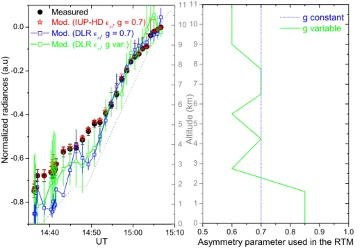
(1) Proceeding as detailed in Sect. 2.3.1, IUP-HDEM is inferred from the (relative) radiances at 353 nm measured during the ascent starting at 14:30 UT. Aerosol opti-cal parameters considered for that retrieval are the phase function, herein simplified
10
as Henyey-Greenstein’s (Henyey-Greenstein, 1941) withg=0.7, and̟0=99%. These
assumptions are based on measurements of microphysical and radiative aerosol prop-erties performed during the ASTAR 2007 (e.g., Ehrlich et al., 2008; Lampert et al., 2009).
(2) The DLREMfrom the PCASP-100X and FSSP-300 measurements is determined
15
during a number of constant level flight legs (e.g., Weinzierl et al., 2009). For this, aver-aged particle size distributions are derived assuming a refractive index of an aver-aged am-monium sulfate type of aerosol. In addition, absorption by particles in the tropospheric aerosol column is assumed to be negligible (i.e., 1.54+0.0i). The scattering (extinc-tion) coefficient is then determined using a Mie model assuming spherical particles.
20
A complete time series (or vertical profile) of scattering/extinction coefficients along the flight is constructed from the aerosol surface area concentrations following from the DLR probes measurements, using the average ratio of scattering coefficient and sur-face area density in the constant altitude flight legs. Three vertical profile scenarios are obtained then: (a) a clean case scenario representing the lowest concentrations
25
per altitude bin over the entire flight, (b) a case for the particular ascent profile flown at around 14:30 UT, and (c) a case scenario representing the few pollution layers found during the flight. In the DLREM retrieval major uncertainties are introduced with the
AMTD
3, 3925–3969, 2010Aircraft-borne DOAS limb measurements
C. Prados-Roman et al.
Title Page
Abstract Introduction
Conclusions References
Tables Figures
◭ ◮
◭ ◮
Back Close
Full Screen / Esc
Printer-friendly Version Interactive Discussion
Discussion
P
a
per
|
Dis
cussion
P
a
per
|
Discussion
P
a
per
|
Discussio
n
P
a
per
|
the variability of atmospheric conditions during the flight. These uncertainties are not further discussed since this exercise only aims for a qualitative comparison of IUP-HD
EM and DLREM.
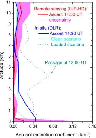
InferredEMvertical profiles (1) and (2a–c) are compared in Fig. 5, where the vertical
resolution of the in situ data has been adopted to the rather coarse resolution of the RT
5
model. As seen in Fig. 5, IUP-HDEMtends to a rather clean scenario above the first 500 m up to the UT/LS. In fact, below 6 km altitude, IUP-HDEM points to an aerosol
load even lower than the “cleanest” in situ measured values.
In order to investigate likely causes for these differences and their consequences for the 14:30 UT EM inferred profiles (see Fig. 5), sensitivity tests are performed for 10
different parameters.
The most sensitive parameter for the RT in the BL appears to be the ground albedo. By analyzing Fig. 5, if a 20% uncertainty of the ground albedo is assumed, the inferred IUP-HD EM vertical profile shows an averaged 200% relative error in the very first
layers of the BL (see pink shadow). Nevertheless, as seen in the figure, uncertainties
15
in the ground albedo do not cover the differences between bothEMprofiles.
Sensitivity studies indicate also that, for the selected spectral range, the inferredEM
may only weakly depend on wavelength (by less than 5%).
Assumptions regarding optical properties of the aerosol particles may also cause the differences. The IUP-HD EM represents an effective extinction coefficient profile 20
constrained to one single type of aerosol (optically described byg=0.7 and̟0=99%).
Conversely, the in situ probes collect data from (optically) different aerosol types that likely coexist in the atmosphere. The single scattering albedo considered in both ap-proaches differs in only 1%. Thus̟0is not considered the optical parameter directing
the differences between IUP-HD and DLR EM. On the other hand, sensitivity stud-25
ies (Fig. 6) indicate that modeling the relative radiances considering DLR EM in the
AMTD
3, 3925–3969, 2010Aircraft-borne DOAS limb measurements
C. Prados-Roman et al.
Title Page
Abstract Introduction
Conclusions References
Tables Figures
◭ ◮
◭ ◮
Back Close
Full Screen / Esc
Printer-friendly Version Interactive Discussion
Discussion
P
a
per
|
Dis
cussion
P
a
per
|
Discussion
P
a
per
|
Discussio
n
P
a
per
|
Bearing all these considerations in mind, a quantitative comparison of theEM
pro-files inferred from both approaches should be regarded with caution. Furthermore, the uncertainties afore mentioned may also indicate the restriction of our aerosol inversion. If the retrieval was not limited by the information content of the measurements, a more detailed remote sensed characterization of the aerosol optical properties could be
per-5
formed, e.g., by an aerosol EM inversion not constrained to one type of aerosol, by taking into account possible 3-D effects, by analyzing the rotational Raman scattering (Ring effect, e.g., Wagner et al., 2009b), and by including the polarization of light in the algorithm (e.g., Emde et al., 2010). Moreover, the retrieval of aerosols from measured
relative radiances may also be combined with O4 d τ measurements to gather more
10
information of the optical properties of aerosols in the lower troposphere. Nevertheless the information content limits the retrieval and, therefore, such a detailed characteriza-tion of aerosols is out of the scope of this work.
Since a self-consistent treatment of the RT is required throughout each of the steps of the retrieval algorithm, Fig. 6 also indicates the limitation of using DLREM as a RT
15
forward parameter for the inversion of the trace gas profiles (see also Fig. 7, center). Hence, the inferred IUP-HD EM profile (constrained to a constant g and ̟0) should
be regarded as an effective 1-D aerosol extinction profile describing the Mie scattering processes in the 1-D atmosphere. The characterization of the RT with this approach is validated in the following section.
20
3.3 Validation of the retrieval of the tropospheric trace gas vertical profile: O4regularization
One of the first steps in our trace gas retrieval method is to choose an atmospheric vertical grid that fits the information content of the measurements. Considering the speed of the aircraft and the integration time of our spectra during the aircraft ascent of
25
AMTD
3, 3925–3969, 2010Aircraft-borne DOAS limb measurements
C. Prados-Roman et al.
Title Page
Abstract Introduction
Conclusions References
Tables Figures
◭ ◮
◭ ◮
Back Close
Full Screen / Esc
Printer-friendly Version Interactive Discussion
Discussion
P
a
per
|
Dis
cussion
P
a
per
|
Discussion
P
a
per
|
Discussio
n
P
a
per
|
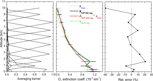
measured data at a given layer (depending also on the regularization strengthα). Following Eq. (6) and using the L-curve criterion to define the regularization pa-rameter α (see Sect. 2.3), the inversion of the O4 vertical profile constrained by the
inferred IUP-HD EM vertical profile (Fig. 5) is performed. Figure 7 characterizes the
O4 profile retrieval at 360.8 nm. As shown by its kernel matrixA (Fig. 7, left), in the
5
retrieval of xreg roughly 8 degrees of freedom are obtained. Since A gives the sen-sitivity of the retrieved profile to the true state, an averaging kernel smaller than unity indicates the limitation of the measurements to provide fully independent information of the true statex. Therefore, the effective null-space contribution is not negligible. Since
xreg=Ax+error and the true O4 state (x) is given by Eq. (1), the retrieval error can be
10
estimated. Figure 7 (center) showsx(blue),Ax(red) andxreg(and covariance, black) for the retrieval of the O4extinction coefficient profile using the aerosol IUP-HDEMas
a forward parameter in the RT model. For comparative purposes, Fig. 7 (center) also shows (in green) the regularized O4 profile constrained by theEM profile as inferred
from aerosol concentrations in situ measured (in dark blue in Fig. 5). Figure 7 (right)
il-15
lustrates the relative error of the O4retrieval (constrained by IUP-HDEMprofile). In the
troposphere (up to 8.5 km), the retrieval of the O4vertical profile shows a good agree-ment with the true state, with a maximum relative error of 20%. This error is mostly dominated by the error in the forward RT model (i.e., coupling of ground albedo and aerosol load uncertainties), which can be understood as a miscalculation of the light
20
path in a given layer. On the other hand, in regions where trace gas concentrations are close to the detection limit of the instrument (e.g., O4in the UT/LS), the retrieval noise
(the measurement error) dominates the total error of the retrieval.
4 Results and discussions
Since in the previous sections the robustness and consistency of the retrieval algorithm
25
AMTD
3, 3925–3969, 2010Aircraft-borne DOAS limb measurements
C. Prados-Roman et al.
Title Page
Abstract Introduction
Conclusions References
Tables Figures
◭ ◮
◭ ◮
Back Close
Full Screen / Esc
Printer-friendly Version Interactive Discussion
Discussion
P
a
per
|
Dis
cussion
P
a
per
|
Discussion
P
a
per
|
Discussio
n
P
a
per
|
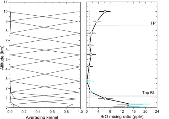
Therefore we proceed to retrieve the targeted vertical tropospheric profile of BrO in the Arctic spring (Fig. 8). Overall, the inferred BrO profile appears to be C-shaped, having three distinct regions: the BL with high BrO mixing ratios (around 15 pptv), the free troposphere with BrO mixing ratios close the detection limit (∼1.5 pptv), and the UT/LS where the BrO mixing ratios increase with altitude. As indicated by the
5
averaging kernels (Fig. 8, left panel), the inferred BrO tropospheric profile has roughly 10 degrees of freedom with an altitude resolution of about 1 km.
Before the discussion can address further details of the inferred BrO profile and inter-comparisons with other studies can be made, specific aspects of our technique and potential implications for the inferred BrO need to be discussed.
10
Since there is a very small contribution of the true state to the null-space (averaging kernels very close to unity throughout the whole profile, Fig. 8, left), the regularized BrO profile presented in black in Fig. 8 (right) is a reasonably good but smoothed approximation of the BrO true state. In the first 1.5 km of the BrO profile (see Fig. 8, right), the forward model RT error is estimated as 80% of the total (black) error, and
15
for the altitudes above, the measurement error dominates (70%) the total BrO retrieval error. Also, the limited height resolution of this aircraft-borne limb technique for trace gas detection – as indicated by the full width at half maximum of the averaging kernels – suggests that details of the BrO profile shape within the first half kilometer of the BL are somewhat uncertain. This statement is particularly supported by the scattering due
20
to particles that tend to radiatively smooth the profile shape in that region (Fig. 5). Furthermore, since the aircraft ascent from near the ground into the UT/LS took roughly 30 min and covered a latitude-longitude distance corresponding to 250 km, the profile retrieval inherently condenses information gained from a 3-D plus time measure-ment into a 1-D effective profile. Consequently, sensitivity studies are performed aiming
25
to estimate the horizontal sensitivity of the limb measurements during the aircraft as-cent. For these studies a stratified atmosphere is considered and, thus, the retrieved aerosols (IUP-HDEM) are supposed to have a homogeneous horizontal distribution.
AMTD
3, 3925–3969, 2010Aircraft-borne DOAS limb measurements
C. Prados-Roman et al.
Title Page
Abstract Introduction
Conclusions References
Tables Figures
◭ ◮
◭ ◮
Back Close
Full Screen / Esc
Printer-friendly Version Interactive Discussion
Discussion
P
a
per
|
Dis
cussion
P
a
per
|
Discussion
P
a
per
|
Discussio
n
P
a
per
|
herein studied where, in the viewing direction of the mini-DOAS instrument, no open water (possible convection) was encountered. Main results from these sensitivity stud-ies are: (1) the mini-DOAS instrument collected scattered skylight from a volume of air that (horizontally) extended 10 to 40 km from left side of the aircraft, (2) the Rayleigh scattering by air molecules dominates over particle scattering when the aircraft
as-5
cended from the BL up to the UT/LS, (3) most of the information gathered comes from the line of sight of the instrument. Some implications of these three findings are given below.
Finding (1) indicates a horizontal sensitivity of the limb measurements of 10–40 km (increasing with altitude). Thus, any small scale variability of the targeted trace gas
10
existing within that distance from the aircraft (depending on the altitude), is in fact av-eraged in our observations. This averaging may not limit the BrO profile retrieval in the free and upper troposphere where a horizontal homogeneity is probably justified. Con-versely, strong BrO horizontal gradients may exist in the BL. In order to study possible BrO horizontal gradients within the horizontal instrument sensitivity range, forward RT
15
analyses are performed. These analyses suggest that, within the first 600 m, the BrO mixing ratio allowing to (independently) reproduce the measured BrO dSCD may be as large as 20 pptv (in cyan in Fig. 8). More insight into the horizontal variability of bound-ary layer BrO mixing ratios may be gained by analyzing the observations during the low level flight passage from 14:10 to 14:35 UT (refer to Fig. 1). This will be investigated in
20
a forthcoming study. Following with the forward RT analyses to study possible BrO hori-zontal gradients above the BL, between 1.2–3 km, the BrO dSCDs measured may also be consistent with BrO mixing ratio of up to 2.5 pptv. Nevertheless, above 3 km, the measurements were not reproducible within the error margins if a steady BrO mixing ratio larger than 3 pptv would be considered in the free troposphere. Moreover,
GOME-25
AMTD
3, 3925–3969, 2010Aircraft-borne DOAS limb measurements
C. Prados-Roman et al.
Title Page
Abstract Introduction
Conclusions References
Tables Figures
◭ ◮
◭ ◮
Back Close
Full Screen / Esc
Printer-friendly Version Interactive Discussion
Discussion
P
a
per
|
Dis
cussion
P
a
per
|
Discussion
P
a
per
|
Discussio
n
P
a
per
|
Finding (2) suggests that the BrO profile retrieved in the UT/LS is independent from the assumption of the horizontal stratification of the aerosols’ optical parameters.
Another critical aspect of the retrieved BrO profiles in the UT/LS (and also of the retrieved IUP-HDEM profile from Fig. 5) addresses a possible contamination of the
measured BrO absorption by photons back-reflected from or near the ground, thus
5
carrying to the location of detection some BrO absorption from the BrO cloud in the BL. However, result (3) suggests e.g. that the BrO profile retrieved in the upper tropo-sphere is not an artifact from BrO enhanced in the BL. This is also confirmed by forward modeling studies which show that the BrO dSCDs measured in the UT/LS can be ex-plained (within the error bars) if no enhanced BrO is considered in the BL. Moreover,
10
the retrieved BrO mixing ratios in the lowermost stratosphere compare well with ex-pectations based on atmospheric BrO profile measurements performed during a large suite of balloon deployments into the lower and middle atmosphere from low, mid and high-latitudes during the past 15 yr (e.g., Weidner et al., 2005; Dorf et al., 2006). Also, since the BrO averaging kernels are very close to unity throughout the whole vertical
15
profile (see Fig. 8), the mentioned BrO surface contamination may be in general ruled out (although the width of the averaging kernel is also to be considered).
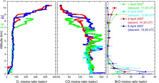
Next the inferred BrO profiles are put in the context of other in situ measured trace gases (O3and CO in Fig. 9). Such an investigation may also assist to test even further
the consistency of the retrieved BrO profile. Figure 9 indicates (in red) that the slightly
20
enhanced BrO found in the upper troposphere could be due to the transport of air masses from the lowermost stratosphere. Hence, this would lead simultaneously to enhanced O3and BrO and to depleted CO. In fact, such transport events (tropopause folds which develop around cut-off lows), are known to occur frequently during the Arctic spring season (e.g, Shapiro et al., 1987; Stohl et al., 2003). These arguments
25
AMTD
3, 3925–3969, 2010Aircraft-borne DOAS limb measurements
C. Prados-Roman et al.
Title Page
Abstract Introduction
Conclusions References
Tables Figures
◭ ◮
◭ ◮
Back Close
Full Screen / Esc
Printer-friendly Version Interactive Discussion
Discussion
P
a
per
|
Dis
cussion
P
a
per
|
Discussion
P
a
per
|
Discussio
n
P
a
per
|
More difficult to discuss are the BrO mixing ratios inferred in the free troposphere. Indeed, there are reports of some pptv of BrO detected in the free troposphere during similar conditions (e.g., Fitzenberger et al., 2000). In addition, the averaging kernels of our BrO retrieval (Fig. 8, left) indicate the independence of the information inferred. Nevertheless, the small BrO mixing ratios close to or at the detection limit (≤1.5 pptv)
5
found for the free troposphere renders it difficult to quantify whether some BrO is actu-ally present. One recent study reports on reactive bromine measurements (HOBr, Br2 and BrO) present in the BL and free troposphere during the Arctic spring of 2008 (Neu-man et al., 2010). In Neu(Neu-man et al. (2010) the amount of reactive bromine was found to be low (≤1 pptv and typically close to detection limit) in the free troposphere.
Photo-10
chemical arguments put forward by the authors (also valid for our conditions) suggest that most (if not all) of the detected reactive bromine was actually HOBr (reservoir) rather than BrO. Since these arguments may also aply for our observations, we can-not conclude that BrO was unequivocally detected in the free troposphere during the ASTAR 2007 campaign.
15
Next the BrO detected within the BL of the Arctic troposphere during spring 2007 is considered (Fig. 9, right). Herein the near surface BrO mixing ratios show strong heterogeneities (with values between 8–30 pptv) with a general trend of decreasing BrO with height. This finding is well in agreement with previous observations of near surface BrO mixing ratios typically high (≥10 pptv) during the polar spring ODEs (e.g.,
20
Hausmann and Platt, 1994; Saiz-Lopez et al., 2007). However, even though in Neuman et al. (2010) BrO is found within our mixing ratio range, their measurements together with photochemical arguments indicate that most of the reactive bromine was actually HOBr (and possibly Br2), rather than BrO. Since herein BrO is selectively detected with
DOAS, their finding of BrO playing a minor role in the total reactive bromine during
25
ODEs somehow contrasts with the overall finding of this work, at least in situations where enough ozone is still available to oxidize the Br atoms formed either from Br2or
AMTD
3, 3925–3969, 2010Aircraft-borne DOAS limb measurements
C. Prados-Roman et al.
Title Page
Abstract Introduction
Conclusions References
Tables Figures
◭ ◮
◭ ◮
Back Close
Full Screen / Esc
Printer-friendly Version Interactive Discussion
Discussion
P
a
per
|
Dis
cussion
P
a
per
|
Discussion
P
a
per
|
Discussio
n
P
a
per
|
Another aspect of the bromine detection may address the variability of BrO in the BL due to the proximity to the open sea, broken sea ice (leads) or closed sea ice. In order to investigate potential source regions of reactive bromine, particular aircraft tra-jectories were planned aiming at flying over these potential sources. As an example, different ascents and descents on 8 April probed the atmosphere over (a) closed or
5
broken sea ice (green, cyan and red profiles in Fig. 9), and over (b) open ocean and scattered sea ice (blue profile in Fig. 9). Worth mentioning is that sensitivity studies in-dicate that heterogeneities in the forward model parameters may affect in unique ways the forward model error (and therefore the total error) for the inferred BrO tropospheric profiles presented in Fig. 9 (right). For instance, the error of the BrO profile at 14:30 UT
10
(in red) is found to be largely determined by the aerosol load. On the other hand, the ground albedo variability dominates the error of the BrO profile at 15:20 UT (in blue). A first inspection of the measured O3, CO and BrO profiles (Fig. 9) reveals that the
largest BrO mixing ratios (up to 30 pptv) were found during the descent over (b) on 8 April (in blue), while the lowest ozone – very close to the detection limit of 3 ppbv
15
(nmol/mol) – was detected during the ascent on 8 April over (a) (in red). Since trans-port and photochemical processes as well as heterogeneous reactions may interact in a complicated manner, for the time being the source region for reactive bromine cannot be concluded as (a) or (b). These facts, together with the sparsity of the collected data and their poor spatial resolution, complicates a firm conclusion on the potential source
20
regions of the reactive bromine. Also a more detailed discussion of observations with respect to the sources of reactive bromine, its atmospheric transport and photochemi-cal transformation is not within the scope of the present study but will require a detailed modeling of the relevant processes. Such an approach is the objective of a forthcoming study.
25
AMTD
3, 3925–3969, 2010Aircraft-borne DOAS limb measurements
C. Prados-Roman et al.
Title Page
Abstract Introduction
Conclusions References
Tables Figures
◭ ◮
◭ ◮
Back Close
Full Screen / Esc
Printer-friendly Version Interactive Discussion
Discussion
P
a
per
|
Dis
cussion
P
a
per
|
Discussion
P
a
per
|
Discussio
n
P
a
per
|
and by the BIRA-IASB/TEMIS groups. The satellite retrievals of both groups are based on a residual technique that combines measured total BrO slant columns and estimates of the BrO absorption in the stratosphere. Furthermore, stratospheric and tropospheric air mass factors are applied in order to account for changes in measurement sensitivity in both stratospheric and tropospheric layers. The BIRA-IASB team applies a
strato-5
spheric correction based on the BrO climatology described by Theys et al. (2009) which uses estimates of the tropopause height (derived from ECMWF data), as well as O3 and NO2 vertical columns simultaneously retrieved by GOME-2 (more details can be
found in Theys, 2010a; Theys et al., 2010b). The MPIC team uses a slightly diff er-ent stratospheric correction by applying a statistical approach which considers O3 as
10
a tracer for stratospheric air masses and assumes a linear relationship between mea-sured O3and stratospheric BrO slant columns. The remaining BrO SCD is considered
to be located in the boundary layer. In contrast to the BIRA algorithm, background BrO in the troposphere is implicitly accounted for in the stratospheric columns and not in the tropospheric estimates (indicated as∗in Table 1).
15
In order to compare the satellite columns with the airborne results, only satellite pix-els with overpasses 30 min before and after the duration of the passages are consid-ered. In addition to the satellite pixels intercepting the Falcon flight track, pixels falling roughly 20 km on the left side of the track (in the mini-DOAS viewing direction) are also taken into account. Adding those pixels parallel to the flight track aim at considering
20
an averaged horizontal sensitivity of the limb measurements throughout the aircraft as-cent. Finally, only the satellite pixels displaying the highest sensitivity to surface BrO have been kept for the comparison.
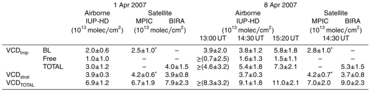
Table 1 provides an overview of the inter-comparison exercise. Shown are the tro-pospheric BrO columns inferred from the flights on 1 and 8 April during the ASTAR
25
satel-AMTD
3, 3925–3969, 2010Aircraft-borne DOAS limb measurements
C. Prados-Roman et al.
Title Page
Abstract Introduction
Conclusions References
Tables Figures
◭ ◮
◭ ◮
Back Close
Full Screen / Esc
Printer-friendly Version Interactive Discussion
Discussion
P
a
per
|
Dis
cussion
P
a
per
|
Discussion
P
a
per
|
Discussio
n
P
a
per
|
lite columns (MPIC and BIRA). Note that no satellite data are given for the 13:00 and 15:20 UT profiles on 8 April 2007, due to the small number of satellite pixels meeting our selection criterion.
As shown in Table 1, within the limits of the experimental errors, the integrated BrO column amounts using the airborne and the satellite approaches compare
reason-5
ably well. Differences between the three groups may be due to different wavelength range chosen for the BrO spectral retrieval (airborne retrieval: 346–359 nm, BIRA: 332–359 nm and MPIC: 336–360 nm), although the possibility that different air masses were sampled cannot be ruled out. On the other hand, deviations between the two satellite retrievals may be attributed to a different choice of the VCD retrieval algorithm
10
(MPIC applies a normalization following the method published by Richter et al. (2002) while the BIRA product does not apply any normalization procedure). Since the ground albedo significantly alters the sensitivity for the satellite detection of trace gases close to the surface, the ground albedo may also play a role in those differences. In these studies, the MPIC group uses the same surface albedo as the mean value used by
15
the IUP-HD group (79%). On the other hand the BIRA group uses variable surface albedo values per pixels, with mean values of 75% (1 April) and 68% (8 April) based on Koelemeijer et al. (2003) climatology. Overall, worth mentioning is also that com-pared to airborne values, the satellite retrieval does not systematically underestimate BrO, a behavior one would expect if the satellite detection of near surface BrO would
20
be systematically obscured in the Arctic, e.g., by scattering due to aerosol and cloud particles.
5 Conclusions
The present study reports on recent developments of aircraft-borne DOAS (Differential Optical Absorption Spectroscopy) limb measurements, the profile retrieval of important
25