MODEL-BASED RUN-TO-RUN OPTIMIZATION FOR PROCESS DEVELOPMENT

of Chemical

Engineering

ISSN 0104-6632 Printed in Brazil www.scielo.br/bjce

Vol. 35, No. 03, pp. 1063-1080, July - September, 2018 dx.doi.org/10.1590/0104-6632.20180353s20170212

MODEL-BASED RUN-TO-RUN OPTIMIZATION

FOR PROCESS DEVELOPMENT

Martin F. Luna

1

_{and Ernesto C. Martínez}

1,

_*

1 _{INGAR (CONICET-UTN), Avellaneda 3657, Santa Fe S3002 GJC, Argentina}

(Submitted: April 21, 2017; Revised: June 26, 2017; Accepted: September 4, 2017)

Abstract - Research and development of new processes is a fundamental part of any innovative industry. For process engineers, finding optimal operating conditions for new processes from the early stages is a main issue, since it improves economic viability, helps others areas of R&D by avoiding product bottlenecks and shortens the time-to-market period. Model-based optimization strategies are helpful in doing so, but imperfect models with parametric or structural errors can lead to suboptimal operating conditions. In this work, a methodology that uses probabilistic tendency models that are constantly updated through experimental feedback is proposed in order to rapidly and efficiently find improved operating conditions. Characterization of the uncertainty is used to make safe predictions even with scarce data, which is typical in this early stage of process development. The methodology is tested with an example from the traditional innovative pharmaceutical industry.

Keywords: Process system engineering; Process development; Experimental design; Modeling for optimization.

INTRODUCTION

Development of innovative processes is a special area of process design that presents an unique feature: knowledge is scarce or inexistent. This implies that the experimental data and the mathematical models are not readily available to be used by engineers and scientists. Some industries require the products to be available as soon as possible in order to get a portion of an emerging market (which shortens the development period) but need the process to be economically viable (making optimization mandatory (Pisano, 1997)). In addition to this, experiments may be expensive to perform in terms of money and/or time, two resources that can be equally valuable. As a result of scarce knowledge, common engineering tasks such as design, control and optimization of industrial processes are carried out under a great deal of uncertainty. The combination of all these features gives rise to a key question to be solved: how to economically develop

an optimal process when knowledge about its behavior and performance is scarce and uncertainty is ubiquitous.

The pharmaceutical sector is a traditional example of an industry that strongly relies on Research and Development (R&D). While historically focused on innovative product development, stagnation in drug discovery and increasing pressure from generic drug producers demand new ways of reducing costs and maximizing returns (Malhotra, 2009). Thus, process development may be the perfect complement for product development. Thousands of drugs are discovered each year, but after a very costly series of experiments (that include from laboratory tests to clinical trials), only a handful of them are selected and approved for their release to the market (Paul et al., 2010). Fortunately for pharmaceutical companies, patent legislation protects drug's inventors, giving them the exclusivity to sell their products (or in the case of novel processes, to manufacture them using

the technology granted in the patent). Nevertheless, patents have expiration dates that make it mandatory for companies to minimize time-to-market in order to maximize sales revenues while their rights are still valid (Minnaard et al., 2007). Also, since different drugs may have the same target market, a fast process development may be needed to increase market share. As a result, shorter development times are needed. On the other hand, as in any other chemical industry, it is desirable that the process behave optimally in terms of yield and productivity in order to meet the market demand at competitive prices (Rubin et al., 2006). This is especially true for drugs such as generics that are no longer protected by patents or those that must compete with biosimilars. More and more pharmaceutical industries that traditionally rely on drug innovation are enhancing their effort on developing more efficient production processes, in order to be able to compete in highly competitive markets with small profit margins (Gernaey et al., 2012).

Since the eighties, the Process System Engineering (PSE) community has studied the problem of process optimization under uncertainty with different approaches (Chen and Joseph, 1987; Filippi-Bossy et al., 1989; Halemane and Grossmann, 1983). With the ubiquitous presence of computers, the model-based optimization approach has gained widespread acceptance. A great deal of effort is being put currently to apply these PSE concepts to innovative industries, such as the pharmaceutical industry (Gernaey and Gani, 2010; am Ende, 2011; Troup and Georgakis, 2013; Royle et al., 2013; Emenike et al., 2015; Rogers and Ierapetritou, 2017). This was reinforced by the U.S. Food and Drug Administration (FDA) with the initiative named Quality by Design (QbD) (ICH Q8, 2006), in which scientific knowledge is used to develop processes that assure quality products. In process development, optimization is usually undertaken when process design has been finished (e.g., the reaction route and separation technology have already been chosen). The purpose of process optimization, then, is to find the best operating conditions (among all feasible ones) that maximize a performance index, subject to process constraints. Among the several PSE optimization approaches, the

modeling for optimization approach aims to solve this problem by developing mathematical models that are used as tools to improve the performance of a process, while interacting with it by performing experiments (Bonvin, 1998; Bonvin et al., 2016).

The combination of model-based optimization techniques and experimental feedback is very useful to overcome the aforementioned difficulties. Since models are constructed with scarce knowledge, their predictions may not be exact, especially when they are used to extrapolate to unexplored process conditions, which may lead to suboptimal results (Quelhas et al., 2013; Mandur and Budman, 2015). To solve this model/ process mismatch, the optimal operating conditions proposed by the model are tested experimentally, and results obtained are used to update the model and improve the performance iteratively, in what is traditionally called a two-step approach. In order to face the problems related to scarce knowledge about processes, probabilistic tendency models (PTMs) are proposed (Martínez et al., 2013), since they take into account the uncertainty associated with predictions at the estimated optimum, which can be very useful to avoid risky or unsafe operating conditions. The tendency of the model refers to its suitability to capture, at least qualitatively, the response of the process to the chosen operating conditions. Both the model itself and its extrapolating capability (the operating region) are corrected iteratively, improving the efficiency of the optimization methodology (Luna and Martínez, 2014). In this work, a methodology to develop novel processes in the face of uncertainty is proposed. In the next section, the modeling for optimization

framework is explained and the probabilistic tendency models are presented. In the third section, the proposed methodology is described and some aspects of its convergence to the process optimum are analyzed. In the fourth section, a typical problem in the pharmaceutical industry (synthesis of an active pharmaceutical ingredient) is addressed. Convergence of the proposed approach is analyzed to highlight its distinctive capability to combine imperfect models with data. Concluding remarks are presented in the last section.

THEORETICAL FRAMEWORK

Modeling for Optimization

maximize a performance index or that minimize a cost, while fulfilling some constraints. The process parameters are the variables of the process that can be specified by the designer, and are confined to the operating region (e.g., reaction temperature, catalyst load, etc.). The process outputs (e.g., reaction yield, production, impurity contents, etc.) are consequences of these parameters. In this work, no process variability is considered in the experiments, i.e., the same process variables give the same outputs in two different experiments (though there may be measurement errors). The traditional formulation of the problem is:

(1)

where J_R is the objective function, C_R(u) are the inequality constraints, D_R(u) are the equality constraints and LB and UB are the lower and upper bounds for the vector of process parameters u. The real optimal operating conditions that solve this problem are denoted u*R. There are several methodologies to optimize a

process and they can be grouped in different ways. Here, optimization approaches are grouped in model-based and model-free methodologies, depending on whether they resort to a mathematical model to represent the process or not. The latter is based mostly on experimentation and a trial & error mechanism (Lundstedt et al., 1998). On the other hand, model-based

methodologies use mathematical models as guidelines to find the optimal operating conditions. This group can be divided as well into two sub-groups. One type is the traditional one-shot optimization methodology, in which all the experimental effort is put into the development of a detailed model, and only after this model is available, is it used to solve the mathematical problem that leads to the optimal operating condition (Franceschini and Macchietto, 2008). The other sub-group of methodologies belongs to the run-to-run (RTR) approach, where the model is developed using a small experimental data set and immediately used to optimize the process (Jang et al., 1987; Chachuat et al., 2009). Since the model could be inaccurate because of the lack of information, the predicted optimum may be suboptimal, so a new experiment is made using the proposed process parameters. Data gathered in the next experiment is then used to update the model, which now will be able to predict better in the neighborhood of the predicted optimum operating conditions. The recursive application of this scheme quickly leads

the process to the high performance area of the design space, avoiding the area of low productivity and reducing experimental costs. The experimental feedback corrects the process/model mismatch and, in so doing, provides convergence to improved operating conditions.

Model-based methodologies rely on the capability of the models to approximate the actual process, at least locally. There are several kinds of process models, but in general, all of them have the form:

(2)

where y is the process output vector, θ is the model parameter vector (the variables that describes the process but cannot be manipulated by the designer) and

u is the vector of parameters that defines the process

operating condition (i. e., the decision variables that the designer can manipulate to optimize the process). The function f is the model, which can be a single equation or a system of equations (algebraic and/or differential) involving even thousands of them. The structure of the model can be based on first principles or entirely based on data, i.e. inductive modeling (Georgakis, 1995). The former uses well-known principles as an efficient way to increase the accuracy of the prediction when extrapolating away from the available data point. The latter use simple mathematical structures to represent the data gathered and are easy to construct, but may fail when extrapolating. Generally, both types of models require a regression of experimental data to find the unknown model parameters (though some processes can be represented by models based solely on constitutive laws).

Using a process model, the real optimization problem can be approximated by:

(3)

where J, C and D are now the model predictions for the objective function, the inequality and equality constraints, respectively. An additional equality constraint on f must be fulfilled, i.e., all variables are

described using the outcomes of y calculated in eq (2), namely the process model. The principal hypothesis is that the predicted optimal vector u* found in problem (3) maximizes both the predicted performance J and the real performance J_R. This may not always be the case, due to the process/model mismatch. Since ( ) . .: ( ) ( ) Max J s t u C u D u LB u UB

0 0 R u R R # # # = ( , ) f y₌ i u

. .: s t Max J

C D

LB u UB

experimentation could be very expensive in terms of money and time in the development of innovative processes, enough experimental data are rarely available and a comprehensive model validation over the entire operating region is usually impossible to perform. Thus, models used for optimization usually have a great deal of uncertainty in their predictions. The information about this uncertainty can be expressed quantitatively using probabilistic tendency models (PTMs): simplified nonlinear models based on first principles which use distributions of parameters (instead of fixed values) that are updated with process feedback (Martínez et al., 2013). In this work, a methodology to optimize an innovative process using PTMs in a RTR scheme is proposed. As is shown below in this work, the speed of the model-based method to find the near-optimal condition, combined with the robustness of the experimental feedback, is instrumental to develop innovative processes.

Probabilistic tendency models

As was stated before, a well-known difficulty in process developments is the lack of experimental data, in quantity (number of experiments) and quality (relevance of the variables measured). Also, the inner mechanism of the process may not be fully known (e.g., the reaction mechanism or the transport phenomena involved in a chemical synthesis). This usually causes a process/model mismatch that may lead to suboptimal operating conditions. The RTR approach may help to overcome this issue, but to do so, some requirements have to be fulfilled. One of these requirements is that the model predicts the tendency of the process. This means that the performance of given (unexplored) operating conditions relative to the performance of known operating conditions (already tried experimentally) is well captured by the model, at least qualitatively. The combination of this concept with the use of well-known first principles and evaluative feedback lead to the development of tendency models. Thus, a tendency model is able to capture the tendency of the process performance, and it is formulated with the objective of optimization (instead of studying the process nature) by successively updating the model parameters.

The PTMs use the bootstrapping method in order to take into account the uncertainty in the prediction due to the scarcity of experimental data. Instead of working with fixed values, the probability distributions of the model parameters are used to characterize the process behavior. The output of the model is not a single value but a distribution, which helps measure the uncertainty of the prediction due to incomplete information.

Before bootstrapping is introduced, a procedure to obtain a parameterization of the model from a single data set is presented. The traditional formulation for model fitting is an inverse problem:

(4)

where E is a function that measures the difference

between the model outputs and experimental data

X. C_θ and D_θ are inequality and equality constraints that can be added to the fitting problem (e.g. to force the solution to accurately predict a specific data point). The experimental data can be taken from one or more experiments, and a single experiment may consist of many data points. The experimental data set X is a subset of all data generated during process development. For the least squares approach, the function E is as follow:

(5)

where the subindex i stands for each element of the data set, u_i is the vector of operating conditions that gives rise to it, y_i is the corresponding model prediction and w is a weighting factor. As can be seen, for given data sets and operating conditions, the solution to the problem is the vector θ of model parameters that minimizes the error function E.

Bootstrapping is a method that generates new artificial data from the original dataset, using re-sampling with replacements (Efron and Tibshirani, 1994; Joshi et al., 2006). Since the model has structural mismatch and measurements have errors, the vector of model parameters that solve problem (4) using the new artificial data set may be different from the one that solves it for the original data set. This process can be repeated until many solutions for problem (4) are obtained. As a result, for each model parameter, there exist different realizations that are considered samples from a distribution (or a histogram), which can then be collected in a stochastic vector iu,, in which every element of the vector is a statistical variable with a distribution. Sampling from these distributions provides a realization of the vector θ_i, which can be used in the tendency model to evaluate a given vector

u, which produces the output y. The procedure can be repeated and the outputs are collected in the stochastic vector

y

u

_{. For example, let's assume that a process}

model output is as follows: . .: s t Max E

C D

LB u UB

0 0 ( , )

( , , )

( , , ) ,u X

u X

u X

#

# #

=

i i

i i

i i

i i

( )

E( , , )u X w yi i( , )u Xi i

2

i

=

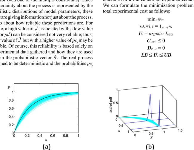
(6)

The stochastic vector iu _{is known and has a normal} distribution with mean 4 and standard deviation 0.5. The output y for each realization θ is calculated at different values of u, and is presented in Figure 1a along with the mean value of y. The scaled probability distribution functions (pdf) are shown for u=0.5 and

u=1 in Figure 1b. Wider distributions imply that the predictions for such values are less accurate.

Since the performance index and the constraints are calculated using y, the following outputs for the probabilistic tendency model can be defined:

(7)

For given vectors of operating conditions u and probability distributions of the model parameters iu r,J is the expected value of the performance index and

pc_j and pd_j are the probabilities that a given inequality or equality constraints are fulfilled (the subindices j

stands for each one of the multiple constraints). Since the uncertainty about the process is represented by the probabilistic distributions of model parameters, these outputs are giving information not just about the process, but also about how reliable these predictions are. For example, a high value of

J

r

associated with a low value of pc_j (or pd_j) can be considered not very reliable; thus, a lower value of

J

r

but with a higher value of pc_j may be preferable. Of course, this reliability is based solely on the experimental data gathered and how they are used to obtain the probabilistic vector iu_{. The real process}

is assumed to be deterministic and the probabilities pc_j

and pd_j do not reflect any perturbations to the process:

experiments are considered are assumed reproducible, though there may exist random measurement errors. The probabilities pc_j and pd_j reflect the remaining

uncertainty about the predictions due to the lack of knowledge about the process.

OPTIMIZATION METHODOLOGIES USING PTMS FOR PROCESS

DEVELOPMENT

Process development methodology

The capability of the PTMs to measure the uncertainty of its own predictions is very useful in the development of new processes. Since it is known that there may be a mismatch between the model and the real process, it is expected that several runs will be needed to achieve near optimal operating conditions. Ideally, the development of a new process should be fast, and most of the runs must be done nearby the optimum, where the cost of sub-optimality is lower. Also, some of the experiments may not fulfill the constraints, making them extremely expensive if the outcomes of a run cannot be exploited economically. We can formulate the minimization problem for the total experimental cost as follows:

(8) ( )

exp y= -1 -iu

Pr Pr J pc C pd D

0 0 ( , )u

J J

J J

( , ) ( , )

( , ) ( , )

u u

u u

# =

= =

i

i i

i i

rr

r r

r r

r r

r r

Q

Q

V

V

. . , ,..., : min

argmax s t i i n

J U

C

D

LB U UB 1

0 0 ( )

( )

( )

( )

U U

i R U

R Ui

R U

i

i

i 6

#

# #

{

= =

=

where U is a matrix in which each row is the vector of process parameters tried in the i-th experiment and φ is the total experimental cost. The latter can be defined in different ways, depending on the characteristics of the process. For example, if the product of the experimental runs can be used or sold, a good definition can be the cumulative difference between the maximum possible benefit and the benefit from each run:

(9)

This is the total performance loss during process development due to suboptimal runs. In other cases, the actual cost of each experiment should be considered (e.g., if the product from each run cannot be used or sold, only costs of experimentation should be accounted for).

As can be expected, the best solution is to achieve the optimal operating conditions in just one iteration, but the required knowledge about the real process behavior to solve problem (1) is not readily available. Thus, problem (1) has to be approximated by a model-based formulation. In this work, an iterative RTR methodology is proposed, but the same formulation for the development problem stands for a one-shot optimization methodology. The main difference is that, for one-shot optimization, some experiments should be performed first to obtain the model and then use it to solve the problem (3), whereas in the RTR approach the model-fitting problem and the optimization problem are simultaneously solved over a number of iterations. As a result, the run-to-run methodology tends to perform most of the experiments in profitable operating conditions, avoiding the low performance areas that may be needed to fit and validate comprehensively the more detailed models used in one-shot optimization. Also, the latter approach relies solely on the model and has no feedback from the real plant once the optimization problem is solved. This may lead to suboptimal operating conditions when there is mismatch between the model and the real process.

There are several RTR methodologies that can be applied to solve the development problem. The traditional approach is to perform an experiment, solve problem (4) to update the model, and solve problem (3) using it. The optimal operating conditions obtained are tested experimentally, and a new iteration begins. This procedure can be repeated until convergence. This is known as the two-phase approach.

In this work, the two-phase approach is combined with a probabilistic formulation that uses PTMs to take

into account the information about the uncertainty of the process. The model-based optimization problem is reformulated as follows:

(10)

where

J

r

_{, pc}

j and pdj are calculated with eq (7).

This formulation is equivalent to the probabilistic programming formulation, which is well known in the fields of stochastic programming (Sahinidis, 2004). One of the main advantages of this formulation is that, by adjusting the parameters α_j and β_j, the user tunes the methodology in accordance with how risky he/ she wants it to be. Higher values of these parameters make the procedure more conservative, as the obtained solution minimizes the probabilities of not fulfilling the constraints. If the true optimum is near or on one (or more) of the constraints, the methodology will slowly move towards it, thus requiring more runs. Lower values, on the other hand, could lead to faster convergence, but at the risk of some unprofitable runs.

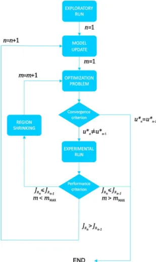
This formulation is implemented in a two-step methodology (Figure 2), where the model acquisition step is performed via regression and bootstrapping and the optimization step is replaced by problem (10). Data from all or some previous experiments can be employed to fit the PTMs, but in this work only data from the last successful experiment are used. Thus, the model is not required to fit data with lower performances that may hamper its predictions in the high-performance region. This is especially true for imperfect models. For complex models, data from other experiments may be included in order to give some information of regions with low performance.

The solution of the optimization problem is the proposed optimal vector u* that has to be tested experimentally. A run is performed using these operating conditions, and if the performance improves, a new iteration begins. If the proposed operating conditions from the new iteration are nearly equal to the one from the last iteration, the development procedure stops and they are considered optimal. A performance increase in the experimental run involves an improved value of J_R while fulfilling C_R and D_R, according to problem (1).

If the performance does not improve, several approaches can be followed. Here, it is proposed that the optimization problem is performed once again using

. .: max

s t J

pc pd

LB u UB

( , )

( , )

( , )

u u

j u j

j u j

$

$

# #

a b

i

i

i

rr

r

r

( ) JR u( ) J uR *R i

i

-the proximity of -the conditions where it was obtained and becomes worse as it is used to extrapolate far away from that point. If the model successively fails to propose better operating conditions, the region shrinking will eventually force the optimization problem to choose the same (or sufficiently similar) operating conditions, thus converging. If improved operating conditions are found, the region is reset to the original values and a new iteration begins from the new conditions. The reset of the bounds may lead to a higher number of experiments until convergence is achieved, but it is done in order to prevent excluding an operating region where the actual optimum may be found. The assumption made is that the newly parameterized model would circumvent the region of low performance without resorting to more restrictive bounds.

An iteration (labeled n) in Figure 2 is defined as

the complete cycle of model fitting along with one or more optimization steps with shrinking. Each iteration may involve several experiments (using m to count the number of experiments in a given iteration). Since it could be very expensive to perform many experiments, a maximum number of experiments per iteration (m_MAX) can be specified as an alternative stopping criterion. In this case, the best operating conditions among all tested are chosen as the optimal. A simple algorithm to shrink the operating region is proposed in Figure 3, where sf is the shrinking factor and u₀ is the operating point where the model was fitted: the best run from the last iteration (or the exploratory run); it is up to the user what value of sf to choose. The lower its value, the smaller the operating region, hence the methodology will be more conservative, meaning the optimization problem is solved in a smaller region.

Figure 2. Block diagram for the optimization scheme proposed in this paper.

the same PTM but in a smaller region, excluding the tested operating conditions u*. As a result, the search region is shrunk around the operating conditions where the model was last fitted. This is in accordance with the belief that the model provides a good tendency in

The procedure is depicted in Figure 4. For a process with two variables, the contours of the performance index J_R for the real process are shown with black lines. The predictions of the tendency model

J

r

fitted with

data from u₀ are presented with dotted lines. The initial optimization region is the whole domain presented in Figure 4a. As can be seen, the performance of the optimum predicted by the model,

u

*

1, is lower than the one from u₀. The shrinking of the optimization region, which is delimited by the dashed lines in Figure 4b, excludes

u

1* such that the new model-optimized process parameter vector

u

*

2 leads to an improvement. Convergence Analysis

To analyze the convergence of the proposed methodology, let's consider the operating point u₀

where the model was last fitted. Let's denote by Nu₀

the neighborhood of u₀ defined as follows:

(11)

where δ is a real number greater than 0 and sufficiently small. The model fits well the process if its predictions and the real process responses are approximately equal, so that:

(12)

It is intuitive that, if the model fits well in the neighborhood of u₀ for a constrained optimization problem which boundaries are within Nu₀, the

optimum predicted by the model and the real one nearly coincide:

(13)

such that their performance indices verify J_R(u*)

≥ J_R(u₀). Since the shrinking methodology reduces the optimization region around u₀, after performing some experiments with a J_R(u) lower than J_R(u₀), the optimization region is included within the neighborhood of u₀. Then, the model-based optimization problem will find a solution u* with a better performance than u₀ (or a comparable performance in the case of convergence). However, it is worth noting that u* is an optimum for the "shrunk" problem, but not necessarily for the real problem. With this operating point as the new model-optimized process parameter vector u₀, a new iteration may be undertaken. As process performance is improved in each one of the iterations, eventually an optimum will be reached for the real problem (there is no guarantee that this is the global optimum, though, as expected in any optimization method that deals with process-model mismatch).

Asking a model to predict correctly all the outcomes of a process for any operating condition could be very challenging. To relax somehow the requirement for a model used for process optimization, the following sub-domain is defined as the "region of improvement" of u₀:

(14)

Figure 4. Contour levels for the real performance (black lines), the prediction of the tendency models (doted lines) and the operating conditions (a) for the first run of an iteration and (b) for the second run, after the region is shrunk.

Nu0=FRu u-u0 1dWI

( ) J J

u

C C

D D

( ) ( )

( )

( ) ( )

u R u

R u

u R u

.

.

.

J J u* u*

( ) ( )

R u R u

R

* R

.

=

A model has good tendency if it can predict, for a given u₀, whether or not an operating condition vector

u fulfills:

(15)

If a model has good tendency, then the predicted optimum u* will have a better performance than u₀, i.e. J_R(u*) > J_R(u₀). However, this does not imply that the performance of the predicted optimum corresponds to the performance J_* of the real optimal operating conditions, i.e., not necessarily J_R(u*) = J_*. If the model has a good tendency nearby u0 and the optimization region is shrunk enough, then eventually the boundaries of the optimization problem must be within the region of improvement and J_R(u*) > J_R(u₀). Tus, if the model has a good tendency in the proximity of any operating condition used such as u₀, then each iteration of the methodology will find an operating condition vector with a better performance. This is important because it is easier for a model to have a good tendency than to fit well.

For the conceptual example presented in this section, the real ROI and the one predicted by the model are shown in Figure 5a and Figure 5b, respectively. In the region where both ROI don't overlap, the model doesn't have a good tendency. As can be seen in Figure 5c, the first proposed optimum

u

*

1 is in this region; thus, the performance of the process decreases. After the operating region is shrunk, the new optimum

u

*2 is predicted in a region where the model has good tendency and the performance improves. Then,

u

*2 becomes the new u₀ and a new iteration begins. Even when the methodology doesn't need to shrink the operating region to the neighborhood of u₀ to achieve better performance, the model has a good tendency in that region as is shown in Figure 5d, which ensures performance improvement.

CASE STUDY

Problem statement

The proposed methodology for the development of a new process will be tested via simulation of the chemical synthesis of an active pharmaceutical ingredient (API). This is a typical problem in the pharmaceutical industry, where a significant number of new drugs are discovered every year but only a few make it to the clinical trials.

The example is rather simple to be easily understood and analyzed, but interesting enough to

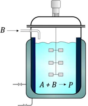
highlight the capabilities of the proposed approach. The reaction scheme is presented in Figure 6. An API (labeled as P) must be synthesized from two reagents (A and B) in a tank reactor. The reaction takes place in the presence of a catalyst and a solvent. The reaction system is complex: after the reaction of A and B and the formation of P, the reaction of P and B can take place leading to the destruction of the product and thus reducing the desired product yield. Also, A and B can follow a parallel reaction path to form an impurity

I. This impurity is very undesirable because at a certain concentration it becomes unstable in solution, precipitates and spoils the batch.

Yield and the impurity issues are both believed to be caused by resorting to an excess of B, thus, a fed-batch operation mode where a solution of B is fed to the solution of A charged initially in the reactor, is selected (Figure 7 describes the setup). After a given time, the reaction is stopped, and the mixture is discharged to the purification step, where the product can be separated. Some assays on laboratory scales are used to define the bounds for the operating conditions. The feeding profile of B should be optimized, leaving all other process variables (temperature, initial volume and reactant concentrations, etc.) at their nominal values. Here the profile is arbitrarily chosen to be a single step described by two parameters:

(16)

where F(t) is volumetric flow and t is time. This is done for the sake of simplicity, because in this way the results obtained with the methodology are easier to analyze (other process variables or more complex feeding profiles may be proposed, if the tendency model is able to represent appropriately the influence of each variable on the process performance). Model simulations are performed using this reaction scheme and reactor setup. The complete set of differential equations used for data generation of the API process can be found in the Appendix. It is worth noting that this complete model and its parameters are unknown to the user.

An intermediate species M is formed, but it cannot be measured experimentally. Actually, the only species that are measured along a production run are P and I. Two constraints need to be fulfilled: the

concentration of I must be less than the maximum allowable concentration of 0.01 mol/L (so as to prevent precipitation) whereas the final volume of the reactor cannot exceed the maximum capacity of the vessel, which is 2.25 L. These constraints are named C₁ and ROI

ue ( )u0

Figure 5. (a) Actual region for process improvement; (b) model predictions for performance improvement; (c) Region where the model doesn't have a good tendency; (d) Zoom of the region around operating conditions used for model fitting.

Figure 6. Reaction scheme for the case study.

C₂, respectively. The exact results of the simulation are perturbed with a 5% Gaussian white noise for data sampled during the experiment, but are considered exact for values at the final time (the measurement at the final time are done offline, with a more accurate

analytical method). The performance index to be optimized is the profit of the run, measured relative to the price of one mol of A:

(17.a)

If the constraint C₁ is not fulfilled, the value of J_R is given by:

(17.b)

because the spoiled product has no value and has to be disposed. The coefficients 4 and 0.3 stand for the relative prices of P and B; B_in is the concentration of B

in the feed stream and V stands for the reactor volume. .

JR=4P V( )tf ( )tf -A V( )0 ( )0 -0 3B u uin 1 2

.

Figure 7. Reactor setup for the case study.

Both A₍₀₎ and B_in are set to 1 mol/L, and V₍₀₎ is 1l. The duration of the experiment t_f is fixed to180 min.

The contour lines of the response surface of the process performance using simulations are presented in Figure 8. Dashed lines describe the constraints. As can be seen, the behavior is highly nonlinear, and the optimum lies on the constraint for I. Also, the feasible region is non-convex, which makes the problem more difficult to solve. The true optimum is located at

u

*

R

_$

= [8.59E-03 L/min, 128.69 min], and

its performance is J_* = 1.4250.

Based on available knowledge about the reaction mechanism, the reaction scheme presented in Figure 9 and the corresponding tendency model presented in eq (18) and eq (19) are proposed (one of the stoichiometric factors should be adjusted experimentally).

(18)

(19)

The parameters to be fitted are the three kinetic constants (k₁, k₂ and k₃) and the coefficients ν and γ.

Figure 8. Contour lines of the performance index and its restrictions for the example presented in this section.

r k AB r k PB r k AB

1 1

2 2

3 3

= = = c

( ) dt

dA _{r r} VFA dt

dB _{r r r}

VF B B dt

dP _{r r} V F_P

dt dI _vr

V F_I

dt dV _F

2 i

1 3

1 2 3

1 2

3

=

-=- - - +

-=

-=

-=

The performance index and constraint C₁ must be obtained using the tendency model, while constraint

C₂ can be exactly predicted a priori since the initial volume is known and the total volume fed is easily calculated from the process parameters vector. The performance index to be optimized in the model-based problem is equal to the one from eq (17.a), because the disposal of the product due to an excess in the impurity concentration is enforced by constraint C₁.

Since constraint C₁ is model-based, and the success of the run depends heavily on its fulfillment, a special constraint in the model fitting problem is added:

(20) By enforcing eq (20), the model is forced to fit accurately the final data point for the impurity concentration.

Samples must be taken during the experiments to make room for fitting model parameters. Since it is a dynamic experiment, this can be done during the run at different times. These measurements of P

and I at different times made up the data set X used to fit the tendency model, but only the final time data

D , ,u X I( )t I( )t exp

f f

=

-i -iR W

point (along with the process parameters and the initial conditions) is used to calculate the performance index. A common practice in the design of dynamic experiments is defining the sampling schedule (Asprey and Macchietto, 2002). This means that the most informative sampling times must be selected instead of choosing them arbitrarily. In this work, this is done using a global sensitivity analysis of the performance index with regards to the model parameters (Saltelli et al., 2006). For more details about these methods the reader is referred to the works of Rodriguez-Fernandez et al. (2007), Luna and Martinez (2014; 2015) and Martinez et al. (2013) and the references therein. Results and analysis

The robustness of the methodology will be tested as the capability to achieve operating conditions with high performance regardless of the starting point and the existence of measurement errors. The following hyper-parameters are chosen: α₁ is chosen to be 50%,

sf is set to 0.5, and m_MAX is equal to 5. The constraint

C₂ is calculated with no uncertainty, thus the value of α₂ corresponds to 100%. Four different starting points are chosen to initialize the procedure. Since measurements have significant noise levels, the same operating conditions in two runs can lead to different parameterizations of the PTM. In order to study the convergence capabilities, the procedure is fully performed several times from different starting points. The parameterization problem and the performance optimization problem are solved using a Successive Quadratic Programming algorithm implemented in MATLAB (function fmincon).

For the starting point ua

0 =[1.20E-02 L/min, 45 min],

data points collected along the exploratory run and the PTM predictions are presented in Figure 10. The pdf for the prediction of I at final time are presented in

Figure 10c. The distribution of model parameters and the sensitivity indices for the first run can be found in the Appendix. The results for all the runs of the first implementation are presented in Table 1.

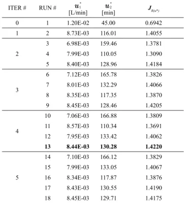
The optimal operating conditions found (Run #13) have a performance only 1% lower than the real optimum. The methodology performed all the experiments in the high productivity region and, in this particular case, none of the runs fail to fulfill the imposed constraints. In Figure 11a, the best run from each iteration is depicted to highlight the performance improvement path. For the second iteration, intermediate runs are shown in Figure 11b, along with the last run from the first iteration. After two attempts that fail, in run #5 the performance does

increase. The obtained operating point is chosen as the new optimum, and the procedure continues from there. The learning curve is presented in Figure 12. The total experimental cost is represented in this figure as the gray area between the learning curve (black line) and the real optimum performance (dashed line).

In order to study the influence of the different parameterizations due to measurement errors, the methodology is applied several times starting from

ua

0. To compare the total experimental cost, the same

number of run must be taken for each application of the methodology, which is chosen here to be 26. For implementations with less runs than the chosen number, the performances of the extra runs are equal to the best run (the optimum). A summary for the different applications is shown in Table 2.

The variability created by measurement errors may affect the efficiency of the procedure, but in all the cases the solution found corresponds to a high performance operating condition. The main difference is in the total experimental cost that increases significantly when a run does not fulfill constraint C₁.

As was stated before, the same methodology is started five times from three other different starting conditions. Results obtained are listed in Table 3.

As can be seen, most of the times the methodology finds near optimal operating conditions. The greatest differences are in the number of runs required and in the total experimental cost. Implementations that start from ub

0 have bigger difficulties to achieve the high

performance region than the others. This is due to the location of the starting point. This point is the furthest from the high performance region and it is in the vicinity of constraint C₁. As a result, some experiments may be performed in the unfeasible region, increasing the total experimental cost. From a practical point of view, this starting point is not very likely to be chosen because it implies a fast addition of reactant B in a short period of time, which will cause a high concentration of B, which in turn is more likely to produce the impurity, according to the chemical reaction scheme. Nevertheless, it has been included in this analysis to show that even when starting in this type of operating conditions, the proposed methodology is able to improve the performance of the process.

Figure 10. Experimental data points (squares) and PTM predictions for the concentrations of (a) P and (b) I. The pdf of the concentration of species I predicted by the model is depicted in (c).

Table 1. All runs from the first implementation of the methodology.

ITER # RUN # u1*

[L/min] u*

2

[min] JR(u*)

0 1 1.20E-02 45.00 0.6942

1 2 8.73E-03 116.01 1.4055

2

3 6.98E-03 159.46 1.3781 4 7.99E-03 110.05 1.3090

5 8.40E-03 128.96 1.4184

3

6 7.12E-03 165.78 1.3826 7 8.01E-03 132.29 1.4066

8 8.35E-03 117.35 1.3870 9 8.45E-03 128.46 1.4205

4

10 7.06E-03 166.88 1.3809

11 8.57E-03 110.34 1.3691 12 7.95E-03 133.42 1.4062

13 8.44E-03 130.28 1.4220

5

14 7.10E-03 166.12 1.3829

15 7.99E-03 133.05 1.4067 16 8.34E-03 117.87 1.3876 17 8.43E-03 130.55 1.4190

18 8.45E-03 129.71 1.4175

an operating condition cannot be chosen. In order to show the effect of α1, the methodology is implemented

five times, always starting from ua

0 again, setting α

1 at

90%, which is considered a conservative value (while

sf and m_MAX remain unchanged). Then, for the sake of comparison, the same procedure is repeated using the optimization methodology without resorting to PTMs (i.e., by solving problem (3) with a single set of model parameters but using the shrinking methodology proposed). Results obtained are presented in Table 4.

As can be expected, the set of implementations with α₁ equal to 90% has lower experimental costs and slightly lower performance indices. The implementations using a non-probabilistic tendency model perform similarly to the case of α₁ equal to 50%, except in the last implementation, where it has some poor results. It can be shown that if model parameter distributions are symmetrical or nearly symmetrical, then the results using α₁ equal to 50% will be similar to those ones obtained by implementing the methodology without using PTMs. However, if the distributions are asymmetrical, the non-probabilistic tendency models may give rise to exceedingly optimistic predictions and, accordingly, it is more likely to perform some experiments outside the feasible region. A comparison of these two alternatives with the base case is shown in Table 5, featuring the mean values of the total experimental cost and the performance index for all the implementations for each case. An additional index it and the improvement of the performance may be

lower. On the other hand, a lower value of α may be able to find the actual optimum, but at the expense of some off-specification runs. For example, a value of α

Figure 11. (a) Best run from each iteration for the first implementation of the methodology. (b) The last run from iteration #1 and all runs from iteration #2.

Figure 12. Learning curve for the first implementation of the methodology.

Table 2. Summary of the implementations starting from operating point ua

0.

# Number

of Runs u

* 1

[L/min] u*

2

[min] φ JR(u*)

1 18 8.44E-03 130.28 1.2207 1.4220

2 12 7.40E-03 154.22 9.8826 1.3972

3 17 8.28E-03 142.50 12.6217 1.4179 4 25 8.40E-03 134.25 15.8048 1.4227

5 12 8.35E-03 140.41 0.9878 1.4168

is presented: the number of runs that fail to fulfill C₁

so that product obtained has to be discarded. Again, the case of α₁ equal to 90% only fails twice to fulfill

C₁, while the other two cases have a higher number of failures.

CONCLUDING REMARKS

A model-based approach for run-to-run optimization of operating conditions in innovative

Table 3. Summary of the implementations for the starting points b, c and d.

# Number

of Runs u

* 1

[L/min] u*2

[min] φ JR(u*)

ub

0_{= [ 1,8E-02 L/min; 30 min ]}

1 26 8.04E-03 142.64 12.7983 1.4152

2 15 1.29E-02 66.64 24.9766 1.3086

3 14 8.21E-03 149.94 15.3505 1.4084 4 21 7.45E-03 152.47 18.2435 1.4000 5 26 8.10E-03 143.29 21.1343 1.4166

uc

0= [ 3E-03 L/min; 180 min ]

1 14 8.00E-03 141.40 1.6593 1.4157

2 18 8.03E-03 149.61 4.7823 1.4109

3 11 8.06E-03 146.66 1.2879 1.4150

4 16 7.50E-03 158.91 1.6744 1.3989

5 15 7.09E-03 165.13 2.5106 1.3832

ud

0= [ 7.5E-03 L/min; 70 min ]

1 24 8.21E-03 139.96 4.2448 1.4188

2 10 8.01E-03 147.11 1.1983 1.4107

3 7 8.32E-03 137.67 0.9730 1.4197

4 9 8.23E-03 145.83 3.9470 1.4140

5 10 7.92E-03 144.53 4.3775 1.4136

Table 4. Summary of the implementations for α1=90% and without using PTMs.

# Number

of Runs u

* 1

[L/min] u*

2

[min] φ JR(u*)

α1=90%

1 5 9.48E-03 104.16 1.3542 1.4011

2 5 8.29E-03 135.84 0.9026 1.4208

3 5 7.33E-03 142.42 1.6989 1.3873

4 5 8.30E-03 137.74 1.2697 1.4187

5 7 8.41E-03 136.64 6.4228 1.4217

With a non-probabilistic tendency model

1 17 8.11E-03 150.04 6.8170 1.4107

2 13 8.10E-03 134.37 6.6267 1.4157

3 15 7.89E-03 148.85 6.9433 1.4118

4 12 8.44E-03 138.43 6.6060 1.4207

Table 5. Comparison of three cases presented.

Case Number of

Failures Mean φ Mean JR(u*)

α1 = 50% 12 8.1035 1.4153

α1 = 90% 2 2.3296 1.4099

No PTMs 19 11.9227 1.3919

process development has been presented. Probabilistic tendency models are proposed to handle significant levels of uncertainty in process models used as guidelines for performance improvement. The novelty of the proposed approach is shrinking the feasible region for optimization until it is included in the so-called region of improvement (ROI). Accordingly, the notion of "tendency" for an imperfect model used in run-to-run optimization is formally related to the ROI around a model-optimized operating condition. Results obtained for a representative case study of a fed-batch reactor for producing an API demonstrate that the proposed method is both robust to modeling errors and to changes in the operating conditions used to begin the search for optimal operating conditions. With the inclusion of PTMs in the formulation it is up to the user to choose how conservative process development is by considering the uncertainty associated to model predictions. If the budget for process development can afford a bigger experimental cost, then higher performance may be sought. However, if resources are scarce, perhaps the user may prefer to reduce the costs at the expense of some optimality loss. In any case, the proposed methodology has the tools to takes these issues into account.

ACKNOWLEDGMENT

The authors would like to thank the Consejo Nacional de Investigaciones Científicas y Técnicas (CONICET) for their financial support.

NOMENCLATURE Optimization problem variables

J Performance index

E Error function

u Process parameter vector (or policy vector)

C Inequality constraint vector

C Equality constraint vector

LB Lower bound vector

UB Upper bound vector

θ Model parameter vector

,

J

i

u r

_{Expected value of the performance index}

pc_j Probabilities of fulfilling an inequality constraint j pd_j Probabilities of fulfilling an equality constraint j

θ̃ Model parameter distribution vector

φ Total experimental cost

ROI Region of improvements f Shrinking factor

m_MAX Maximum number of experiments per iteration

Process variables

F Volumetric flow rate [L.min-1_]

A Reagent A concentration [mol.L-1_]

B Reagent B concentration [mol.L-1_]

I Impurity I concentration [mol.L-1_]

P Product P concentration [mol.L-1_]

V Liquid volume [l]

B_in Concentration of B in the inlet flow [mol.L-1_]

r_j Rate of the j-th reaction [mol.L-1_.min-1_]

k_j Kinetic constant of the j-th reaction

ν Stoichiometric coefficient for the third reaction

γ Exponential factor for the third reaction

t Time [min]

t_f Final time or duration of the experiment [min]

Subscripts and superscript

R Real process

θ Relative to a parameter setting

* Optimal

exp Experimental

REFERENCES

amEnde, D.J., Chemical Engineering in the Pharmaceutical Industry: R&D to Manufacturing. John Wiley & Sons: New Jersey, 2011.

Asprey, S.P., Macchietto, S., Designing robust optimal dynamic experiments. J Process Control, 12(4), 545-556 (2002).

Bonvin, D., Georgakis, C., Pantelides, C. C., Barolo, M., Grover, M. A, Rodrigues, D., Schneider, R., Dochain, D, Linking Models and Experiments. Ind. Eng. Chem. Res., 55(25), 6891-6903 (2016). Bonvin, D., Optimal operation of batch reactors-a

personal view. J Process Control, 8(5-6), 355-368(1998).

Chachuat, B., Srinivasan, B., Bonvin, D., Adaptation strategies for real-time optimization. Comput. Chem. Eng., 33(10), 1557-1567 (2009).

Chen, C. Y., Joseph, B., On-line optimization using a two-phase approach: an application study. Ind. Eng. Chem. Res., 26(9), 1924-1930 (1987).

Emenike, V. N., Schenkendorf, R., Krewer, U., A systematic reactor design approach for the synthesis of active pharmaceutical ingredients. European Journal of Pharmaceutics and Biopharmaceutics.

In Press. (2017).

Filippi-Bossy, C., Bordet, J.,Villermaux, J., Marchal-Brassely, S., Georgakis, C., Batch reactor optimization by use of tendency models. Comput. Chem. Eng., 13(1-2), 35-47(1989).

Franceschini, G., Macchietto, S., Model-based design of experiments for parameter precision: State of the art. Chem. Eng. Sci., 63(19), 4846-4872 (2008). Georgakis, C., Modern tools of process control: The

case of black, gray & white models. Entropie, 31(194), 34-48 (1995).

Gernaey, K. V., Gani, R., A model-based systems approach to pharmaceutical product-process design and analysis. Chem. Eng. Sci., 65(21), 5757-5769 (2010).

Gernaey, K. V., Cervera-Padrell, A. E., Woodley, J. M., A perspective on PSE in pharmaceutical process development and innovation. Comput. Chem. Eng., 42, 15-29 (2012).

Halemane, K. P., Grossmann, I. E., Optimal process design under uncertainty. AIChE J., 29(3), 425-433 (1983).

ICH Q8 - Food and Drug Administration CDER. Guidance for industry, Q8 pharmaceutical development (2006).

Jang, S. S., Joseph, B., Mukai, H., On‐line optimization of constrained multivariable chemical processes. AlChE J., 33(1), 26-35 (1987).

Joshi, M., Seidel-Morgenstern, A., Kremling, A., Exploiting the bootstrap method for quantifying parameter confidence intervals in dynamical systems. Metab. Eng., 8(5), 447-455 (2006). Luna, M. F., Martínez, E. C., A Bayesian approach to

run-to-run optimization of animal cell bioreactors using probabilistic tendency models. Ind. Eng. Chem. Res., 53(44), 17252-17266 (2014).

Luna, M. F., Martínez, E. C., Run‐to‐Run Optimization of Biodiesel Production using Probabilistic Tendency Models: A Simulation Study. Can. J. Chem. Eng., 93(9), 1613-1623 (2015).

Lundstedt, T., Seifert, E., Abramo, L., Thelin, B., Nyström, Å., Pettersen, J., Bergman, R., Experimental design and optimization. Chemometr. Intell. Lab., 42(1-2), 3-40(1998).

Malhotra, G., Rx for Pharma. Chem. Eng. Prog., 105(3), 34-37 (2009).

Mandur, J. S., Budman, H. M., Robust Algorithms for Simultaneous Model Identification and

Optimization in the Presence of Model-Plant Mismatch. Ind. Eng. Chem. Res., 54(38), 9382-9393 (2015).

Martínez, E.C., Cristaldi, M.D., Grau, R.J., Dynamic optimization of bioreactors using probabilistic tendency models and Bayesian active learning. Comput. Chem. Eng., 49, 37-49 (2013).

Minnaard, A. J., Feringa, B. L., Lefort, L., De Vries, J. G., Asymmetric hydrogenation using monodentatephosphoramidite ligands. Acc. Chem. Res., 40(12), 1267-1277 (2007).

Paul, S. M., Mytelka, D. S., Dunwiddie, C. T., Persinger, C. C., Munos, B. H., Lindborg, S. R., Schacht, A. L., How to improve R&D productivity: the pharmaceutical industry's grand challenge. Nat. Rev. Drug Discovery., 9(3), 203-214 (2010). Pisano, G. P. The development factory: unlocking the

potential of process innovation. Harvard Business Press, 1997.

Quelhas, A.D., de Jesus, N. J. C., Pinto, J.C., Common vulnerabilities of RTO implementations in real chemical processes. Can. J. Chem. Eng., 91(4), 652-668 (2013).

Rodriguez-Fernandez, M., Kucherenko, S., Pantelides, C., Shah, N., Optimal experimental design based on global sensitivity analysis. Comput. Chem. Eng., 24, 63 (2007).

Rogers, A., Ierapetritou, M., Challenges and opportunities in modeling pharmaceutical manufacturing processes. Comput. Chem. Eng., 81, 32-39 (2015)

Royle, K.E., delVal, I.J., Kontoravdi, C., Integration of models and experimentation to optimise the production of potential biotherapeutics. Drug. Discov. Today., 18(23-24), 1250-1255(2013). Rubin, A. E., Tummala, S., Both, D. A., Wang, C.,

Delaney, E. J., Emerging technologies supporting chemical process R&D and their increasing impact on productivity in the pharmaceutical industry. Chem. Rev., 106(7), 2794-2810 (2006).

Sahinidis, N.V., Optimization under uncertainty: state-of-the-art and opportunities. Comput. Chem. Eng., 28(6), 971-983 (2004).

Saltelli, A., Ratto, M., Tarantola, S., Campolongo, F., Commission, E. Sensitivity analysis practices: Strategies for model-based inference. Reliab. Eng. Syst. Safe., 91(10-11), 1109-1125(2006).

The following equations are used to simulate the real process:

(A.1)

(A.2)

r

k A B

r

k P B

r

k A B

r

k M

r

k C B

1 1

2 2

3 3

4 4

5 5

=

=

=

=

=

Appendix. API Model used for simulating experiments.

(

)

dt

dA

r

r

r

_V

F

A

dt

dB

r

r

r

r

r

_V

F

B

B

dt

dP

r

r

V

F

P

dt

dM

r

r

r

_V

F

M

dt

dI

r

_V

F

S

dt

dV

F

i

1 3 4

1 2 3 4 5

1 2

3 4 5

5

= +

-=- - - + - +

-=

-=

-=

-=

The values for the kinetic constants are given in Table A.1.

Table A.1. Parameters used to simulate the experimental data.

Parameter Value

k1 1.225 E-01 [L.mol -1_.min-1_]

k₂ 1.870 E-02 [L.mol-1_.min-1_]

k₃ 7.0 E-03 [L.mol-1_.min-1_]

k4 3.0 E-02 [min -1_]