Development of a cold stage for a 80 K vibration-free cooler

(1)

Miguel Ângelo Gomes Baeta

Licenciado em Ciências da Engenharia Física

Development of a cold stage for a 80 K

vibration-free cooler

Dissertação para obtenção do Grau de Mestre em Engenharia Física

Orientador: Prof. Dr. Grégoire Bonfait,

Professor Associado com Agregação, Universidade Nova de Lisboa

Júri

Presidente: Prof. Dr. Filipe de Oliveira Arguentes: Prof. Dr. Daniel Vaz

(2)

(3)

Development of a cold stage for a 80 K vibration-free cooler

A Faculdade de Ciências e Tecnologia e a Universidade NOVA de Lisboa têm o direito, perpétuo e sem limites geográficos, de arquivar e publicar esta dissertação através de exemplares impressos reproduzidos em papel ou de forma digital, ou por qualquer outro meio conhecido ou que venha a ser inventado, e de a divulgar através de repositórios científicos e de admitir a sua cópia e distribuição com objetivos educacionais ou de inves-tigação, não comerciais, desde que seja dado crédito ao autor e editor.

Este documento foi gerado utilizando o processador (pdf)LA_{TEX, com base no template “unlthesis” [1] desenvolvido no Dep. Informática da FCT-NOVA [2].}

(4)

(5)

Ac k n o w l e d g e m e n t s

A realização desta tese de dissertação não teria sido possível sem o apoio recebido de forma direta ou indireta por parte de um conjunto de pessoas e entidades. Neste sentido, gostaria de expressar o meu profundo agradecimento nas linhas.

Em primeiro lugar gostaria de agradecer ao Professor Grégoire Bonfait pela oportu-nidade que me foi conferida e pela sua excelente orientação, tempo e dedicação despendi-dos.

Agradeço também aos meus colegas do laboratório de Criogenia: Patrícia Sousa, Hugo Rações, Mário Xavier, Diogo Silva, Sofia Alves e com especial destaque para o Jorge Barreto por me terem acompanhado e ajudado no desenvolvimento deste projeto.

Expresso também o meu agradecimento à oficina do departamento, ao Faustino e Eduardo, pela sua assistência e paciência na construção deste projeto.

Agradeço ainda àActive Space Technologiespela sua colaboração, bem como a todos os

elementos desta empresa que participaram neste projeto.

Aqui expresso também o meu agradecimento à gloriosa Faculdade de Ciências e Tec-nologias da Universidade Nova de Lisboa pelos fantásticos 5 anos que conduziram a este momento.

Para concluir, quero deixar aqui um enorme agradecimento à minha família em partic-ular ao meus pais, Isabel Baeta e Paulo Baeta, seu apoio incondicional e esforço para me proporcionarem esta oportunidade. E também um muito obrigado aos meus amigos com destaque para a minha melhor amiga e namorada Inês Maldonado pela força e paciência ao longo desta jornada.

(6)

(7)

A b s t r a c t

Nowadays, many satellites are observing the earth for many purposes (climatology, agriculture, defence and security, etc.) using infrared sensors. One of the key element of these sensors is their high resolution obtained due to their quite low operating tempera-ture provided by mechanical cryocoolers.

However, the introduction of vibrations by the most of the cryocoolers is a recur-ring problem for space applications, and because of that the development of a system that eliminates these vibrations is very important. So, in the framework of a European Space agency project, a 40-80 K vibration-free cooleris being developed that combines

two cryocoolers (one that uses Nitrogen that precool another cryocooler that uses Neon), functioning without introducing vibrations in the system.

This thesis is focused on the nitrogen cryocooler more specifically on the dimen-sioning and development of its cold part’s components as the Joule-Thomson valve, the counterflow heat exchanger, and its test systems.

The majority of the work on this thesis was focused on the design of the Joule-Thomson (JT) valve. Since Its dimensions and properties are empirically obtained, an extended experimental study of the performance of two diff_{erent JT valves under several}

temper-atures, pressures and mass flow conditions was made. The data obtained allowed us to dimension a JT valve for the required conditions and also confirm the operating principles of the cryocooler cold part.

The counterflow heat exchanger was dimensioned, built and integrated in a Giff

ord-Mac Mahon cryocooler and is ready to be tested as soon as the Joule Thomson valve is determined.

(8)

(9)

R e s u m o

Atualmente são inúmeros os satélites que se encontram em observação da Terra, com as mais diversas finalidades (climatologia, agricultura, defesa e segurança, etc.), através do recurso a sensores infravermelhos. Um dos elementos chave destes sensores é a sua alta resolução, esta é obtida devido à sua temperatura de operação bastante baixa, o que é conseguido através da ação de criorefrigeradores mecânicos.

Contudo, a introdução de vibrações por parte da maioria dos criorefrigeradores cons-titui um problema recorrente na área da aeroespacial sendo pertinente o desenvolvi-mento de um equipadesenvolvi-mento que permita eliminar estas vibrações. Assim, encontra-se a ser desenvolvido no contexto de um projeto da Agência Espacial Europeia, o 40-80 K

vibration-free coolerque combina dois criorefrigeradores, um primeiro que utiliza Azoto

que pré-arrefece um outro que utiliza Néon, e que desempenha a sua função sem, no entanto, introduzir vibração no sistema.

Esta tese incidiu no criorefrigerador de azoto, mais especificamente no dimensiona-mento e desenvolvidimensiona-mento de componentes do seu dedo frio como a válvula de Joule-Thomson, permutador de calor de contracorrente e respetivos sistemas de teste.

Foi sobre o dimensionamento da válvula de Joule-Thomson que recaíram a maior parte dos testes realizados, uma vez que este é um tema pouco estudado e que implicou o conhecimento e validação dos princípios de funcionamento desta válvula, tempera-tura, potência frigorífica e fluxo de massa. Após a realização destes testes, conseguiu-se dimensionar a válvula e ainda comprovar os princípios de funcionamento do dedo frio.

O permutador de calor contracorrente foi dimensionado, construído e integrado no criorefrigerador Giff_{orf- Mac Mahon, e encontra-se pronto a ser testado, logo que a válvula}

de Joule Thomson esteja terminada.

(10)

(11)

C o n t e n t s

List of Figures xiii

List of Tables xvii

1 Introduction 1

2 Vibration free coolers 3

2.1 Coolers usually used in satellites . . . 3

2.1.1 Passive Coolers . . . 3

2.1.2 Active Coolers . . . 4

2.1.3 Joule-Thomson sorption coolers: general principles. . . 6

2.2 Applications . . . 7

2.2.1 Planck . . . 7

2.2.2 METIS . . . 8

3 Thermal and Mechanical requirements and adopted solution 11 3.1 Thermodynamic analysis of the cold part. . . 11

3.2 Counterflow heat exchanger . . . 13

3.2.1 Calculation of the pressure drop in HX tubes versus diameter. . . 14

3.2.2 Calculation of the tube thickness . . . 17

3.2.3 Thermal exchange in the HX versus length . . . 18

3.3 Joule-Thomson valve . . . 22

4 Experimental Setup 25 4.1 Experimental setup for the Joule-Thomson valve . . . 25

4.1.1 Manufacturing of the Joule-Thomson system . . . 30

4.1.2 Control and Acquisition System . . . 34

4.1.3 Mechanical tests . . . 35

4.2 Experimental setup for the Cold part . . . 36

5 Results and discussion 41 5.1 Joule-Thomson valve . . . 41

5.1.1 Mass flow . . . 41

(12)

CO N T E N T S

6 Conclusions 51

Bibliography 53

A Appendix 55

A.1 Cold stage system in SOLIDWORKS . . . 56

A.1.1 Drawings . . . 56

(13)

L i s t o f F i g u r e s

1.1 Schematic of the vibration free cooler to be developed in the framework of an ESA project entitled “Development of a 40-80 K vibration free cryocooler”

proposal, AST-FCT, 2014 . . . 2

2.1 Schematic of a sorption cooler . . . 6

2.2 Sorption cooler from Planck[3] . . . 8

2.3 Sorption coolers system from METIS[5]. . . 10

3.1 Nitrogen cold stage . . . 11

3.2 Thermodynamic processes in a PH diagram. The various steps are explained in the text. . . 13

3.3 Counterflow heat exchanger . . . 14

3.4 Moody diagram made by GraphExpert Professional. . . 14

3.5 Graph of the evolution of Reynolds number with diameter . . . 15

3.6 Curve of the evolution of pressure with diameter . . . 16

3.7 Thickness of the high pressure tube vs the inner diameter . . . 17

3.8 Comparison of thin and thick cylinder theories for various diameter/thickness ratios[8] . . . 18

3.9 The temperatures profile inside the heat exchanger using notation of figure 3.3 19 3.10 Plot of the output temperature of the high-pressure pipe with the length in the heat exchanger. . . 20

3.11 Plot of temperature evolution with the length of the heat exchanger . . . 21

3.12 Graph of nitrogen inversion curve on the Joule-Thomson limits the zone of decreasing temperature . . . 22

3.13 Schematic of the Joule-Thomson valve . . . 23

3.14 The Maytal correlation factor[12] . . . 24

4.1 Schematic of the system used . . . 25

4.2 Gas control system assembly . . . 26

4.3 Schematic of the Joule-Thomson system . . . 27

4.4 Plot of the evolution of the temperatures with the length in HX1 . . . 28

4.5 Plot of the evolution of the temperatures with the length in HX2 . . . 28

(14)

L i s t o f F i g u r e s

4.7 The second heat exchanger (HX2) . . . 31

4.8 Images of the 25.05 µmrestriction with SEM from Centro de Materiais da Universidade do Porto (CEMUP). . . 31

4.9 The JT valve assembly. . . 32

4.10 The Joule-Thomson valve overall system . . . 33

4.11 Control and Acquisition devices . . . 34

4.12 Main tab of the LabV IEWT M program. This tab monitors the temperature, pressure and flow rate through the system.. . . 35

4.13 SOLIDWORKS drawing for the cold part of the nitrogem JT system . . . 36

4.14 The counterflow Heat Exchanger during the winding process . . . 37

4.15 The counterflow Heat Exchanger . . . 38

4.16 HX1 and HX2 for this test system and their thermalizations on stage 1 and 2 of the smaller cryocooler. . . 38

4.17 The Counterflow heat exchanger overall system . . . 39

5.1 The mass flow in function of pressure at room temperature for both restrictions using equation 3.22 and REFPROP data with aCd of 100% . . . 41

5.2 The discharge coefficients in function of pressure at room temperature for both restrictions using equation 3.22 and REFPROP data and the dashed lines represents its average value . . . 42

5.3 Interface of theLabV IEWT M during a test system at 38.2 bar and a mass flow of 502 mL/min. Note the stable temperature of 140.86 K achieved before the expansion (violet line) . . . 43

5.4 The mass flow in function of temperature at a pressure of 50 bar to the restric-tion of 49.25µm with aC_d of 89%. . . 43

5.5 The mass flow in function of temperature at a pressure of 60 bar to the restric-tion of 25.05µm with aC_d of 85%. . . 44

5.6 The mass flow in function of pressure at a temperature of 151 K to the restric-tion of 25.05µm with aCd of 85%. . . 45

5.7 The mass flow in function of pressure at a temperature of 141 K to the restric-tion of 25.05µm with aCd of 85%. . . 45

5.8 Comparison of the Maytal’s correction factor Gamma[12] and our results. Black lines: Maytal’s results, red line: 151 K; blue line: 141 K, yellow point: extrapolated and green point Maytal’s result both under our work conditions 46 5.9 Representation of the isenthalpic expansion in the Joule-Thomson valve at 60 bar. . . 47

5.10 Variation of the temperatures during the process used for cooling power (CP) determination (See text) at a pressure and heating power (H3, see figure 4.3) constant. . . 48

(15)

A.1 Overall system . . . 56

A.2 Precooling system and internal interfaces . . . 57

A.3 High pressure interface with the outside of the cryocooler . . . 57

(16)

(17)

L i s t o f Ta b l e s

2.1 Table of cryocoolers often used below 100 K in space cryogenics adapt from [1] 5

3.1 System conditions . . . 12

3.2 Heat exchanger dimensions . . . 21

4.1 Functions of the control and acquisition devices . . . 34

5.1 The predicted diameters for a flow of 23.7 mg/s . . . 46

(18)

(19)

C

h

a

p

t

e

r

1

I n t r o d u c t i o n

In the last years the requirements of the technologies used in space missions have been increasing, which led to the need to improve their performances. In several areas such as detection systems, telecommunications, conservation of samples, etc., this efficiency

can be achieved with the assistance of autonomous cryogenic systems, called coolers, to replace the use of cryogenic liquids. Unfortunately, these systems have some disadvan-tages: for instance, for highly sensitive detection systems, their biggest disadvantage is the introduction of vibrations produced by mechanical compressors, which may cause a decrease of the system quality.

In an attempt to eliminate this problem, European Space Agency (ESA) proposed the development of a 40-80 K vibration-free cooler. One of the two winning proposals was assigned in 2015 to a consortium grouping: a Portuguese company - Active Space Technologies (a company based in Coimbra, that works in diff_{erent areas, such as space,}

aeronautics, nuclear, defense, industry and research), the Cryogenics Laboratory from LIBPhys and the Laboratory of Adsorption Technology & Process Engineering (LATPE, REQUIMTE), both located at the Faculdade de Ciências e Tecnologias, Universidade Nova de Lisboa.

The objectives of this project are the design, construction and validation of a two-stage vibration free cooler, using nitrogen and neon as the working fluids and a Joule-Thonson expansion as cooling source. The cold part of this system, as depicted inside the dashed box on picture 1.1, consists on counterflow heat exchangers, and Joule-Thomson valves. Attached to the cold part is a gas manifold for the gas management and a set of adsorption cells acting as thermal compressors.

(20)

C H A P T E R 1 . I N T R O D U C T I O N

around 40 K, with a cold power of 0.5 W. These two cryocoolers form a vibrationless system due to the absence of moving parts. In the future, the whole system can cool an infrared device for Earth observations in ESA space missions.

Figure 1.1: Schematic of the vibration free cooler to be developed in the framework of an ESA project entitled “Development of a 40-80 K vibration free cryocooler” proposal, AST-FCT, 2014

It is in the framework of this project that this master thesis is included. The work will be focused on developing the first version of the cold part of the vibration free cooler using nitrogen, with a low temperature around 80 K and a cold power of 1.5 W, represented inside the red box on picture 1.1. More specifically, it includes the design and construction of the counterflow heat exchanger and the Joule-Thomson valve. It includes also, the construction of a system to test the operation of the componements and the system requirements.

(21)

C

h

a

p

t

e

r

2

Vi b r a t i o n f r e e c o o l e r s

In this chapter are presented different types of cryocoolers , some of their performances

and limitations are compared as well as the most common applications in order to justify the choice of a Joule-Thomson system.

2.1 Coolers usually used in satellites

The coolers can be divided in two groups, passive and active coolers. The passive cool-ers do not require an electric power supply and have been extensively used in space applications due to their high reliability and low vibrations level.

The active coolers, also called cryocoolers, in contrast with passive coolers, require electrical power. This energy is used to provide work to a closed thermodynamic cycle, which allows the heat absorption and consequent cooling at the "cold finger" level. The work is usually done by a mechanical compressor, which causes vibration in this system and is therefore the biggest disadvantage in some systems. These coolers may also have multiple stages in order to achieve lower temperatures.

The first active cooler successfully operated in space was a Stirling cycle machine to cool two gamma ray detectors, launched in 1978 and developed by Phillips[1].

In addition, as opposed to passive coolers, the active coolers may cover all ranges of temperatures and can work at any orbit.

2.1.1 Passive Coolers

• Radiators

(22)

C H A P T E R 2 . V I B R AT I O N F R E E CO O L E R S

K in the most cases. Beyond their passive characteristic, another main advantage of these systems is their lifetime because their only limitation is the degradation of the surface of the panels, which is, in space very slow. Their major drawbacks is their limiting temperature and their relatively low cooling power below ≈100

K. Moreover, in the case of radiators in orbits nearby Earth it is diffi_{cult to reach}

temperatures below 70K.

• Cryogenic liquids

The working principle of this type of coolers is quite simple. It consists in a liquid reservoir (Dewar) where the heat dissipated by the sensors is transferred to the fluid by keeping objects dipped in the liquid or in thermal contact with the reservoir at temperatures near the boiling temperature of the fluid. The cryogenic liquids are very suitable due to their temperature stability and their simplicity, although they have a main disadvantage, the fact of adding large weight and volume to the system and of having a finite life time associated with the amount of stored fluid. Let us note that many temperature ranges, in particular the 44 - 54 K, are not covered by this type of coolers, due to the absence of pure liquid fluids in that temperature range.

2.1.2 Active Coolers

• Stirling cycle

They are constituted by a compressor and a regenerative heat exchanger, in general, displaceable, also known as regenerator-displacer. This system is known as the Stir-ling cycle, which consists of two isochoric processes and two isothermal processes [1].

• Pulse tube

The Pulse tube cryocooler is also constituted by a compressor, but, in opposite to the Stirling machine, the regenerator is fixed. This fact eliminates all the moving parts at low temperatures and makes these cryocoolers mechanically simpler and with a low level of vibrations at the cold finger. However, it is diffi_{cult to achieve}

high effi_{ciencies close to the values of Stirling in this type of system.}

• Joule-Thomson

The principle of these cryocoolers is based on the Joule-Thomson eff_{ect which}

corre-sponds to an isenthalpic expansion that occurs when a gas is forced to pass through a small restriction with the assistance of a mechanical compressor. Below the inver-sion temperature, that is gas dependent, this expaninver-sion leads to a cooling. However, this process is highly irreversible which makes these cryocoolers relatively ineffi

(23)

(absence of moving parts at low temperature) and because low temperature can be achieved using adequate cryogenic fluids.

• Joule-Thomson sorption coolers

The sorption coolers systems are similar to the Joule-Thomson ones, and are con-stituted by the same components except the source of gas flow: the mechanical compressor is replaced by adsorption or absorption cells. The cells are volumes filled by adsorption or absorption materials, such as activated carbon or metal hy-drides, respectively. When these materials are cooled the gas particles are retained (in surface or in volume) by the material by physical processes, as Van der Waals forces, or chemical processes, usually covalent bonds. When they are heated the particles are released providing the necessary pressure to the system. These cry-ocoolers have a great potential, in spite of having a relatively low effi_{ciency, because}

when the mechanical compressor is replaced, all moving parts of the system are eliminated and consequently also their inherent vibrations. It is a cryocooler of this type that will be developed in this project.

Table 2.1: Table of cryocoolers often used below 100 K in space cryogenics adapt from [1]

Parameters of coolers

Cooler Temperature Advantages Disadvantages

Radiator 80 K Reliable, low vibration, Complicates in orbits long lifetime nearby Earth Cryogenic _{1.8 K} _{Stable, low vibration} Short lifetime, complex,

liquids out-gassing, massive

Stirling _{to 20 K}80 K _{intermediate temperature}Efficient, Vibrations

Pulse tube 80 K Lower vibrations Lower e_{than Stirling}fficiency,

Joule-Thomson 4 K Low vibrations _eficiencyLow

(24)

2.1.3 Joule-Thomson sorption coolers: general principles

Figure 2.1: Schematic of a sorption cooler

The operation of the Joule-Thomson sorption coolers is schematized in figure 2.1and can be divided in several steps:

• Gas supply

The material constituting the absorption cell is the key to the sorption compressor operation. This should be capable of absorbing large amounts of gas at low pres-sure and temperature, and then desorb it when heated, thus providing the high pressure and the mass flow needed by the system. The temperature cycles are made using a heat switch, an electric heater and a heat sink (Radiator, Cryogenic liquid, etc.). When it is necessary to heat the cell, this should be kept thermally isolated (Heat switch open), to cool it is only necessary to couple the cell to the radiator (Heat switch closed), for example. The problem of using a single cell is that it does not provide a continuous cooling due to the adsorption-desorption steps that are necessary to provide the flow in a cyclic way. This problem can be solved by using multiple cells out of phase: through this principle and using one-way valves (check valves) it was possible to maintain a almost constant flow.

• Gas precooler

(25)

• Joule-Thomson valve

After this pre-cooling, the gas flow is forced through a restriction valve, Joule-Thomson valve, which causes an isenthalpic expansion and consequently a decrease

in the temperature and, in general, liquefaction of part of the fluid.

• Evaporator or Cold finger

After the Joule-Thomson valve, a part of the cold fluid pass into the liquid state and is stored in a Liquid Reservoir, being in this location the lowest temperature of the cryocooler which corresponds to the evaporation temperature of the fluid. Liquid Reservoir is also where the heat is transfer to the device and this heat will cause the liquid evaporation. The gas will then return to the compressor by the low pressure side, through the several heat exchangers to be compressed again. That is why this system is a closed cycle and continuous.

2.2 Applications

2.2.1 Planck

The Planck satellite refers to a space mission that ESA launched on 14th May 2009, with the duration of three years. The purpose of this mission was to study the expansion of the universe by measuring with high precision the anisotropy of microwave radiation on space background.

The microwave measuring system was designed to measure frequencies between 30 and 957 GHz. To cover this frequency range it was necessary to divide the system in two devices, one for lower frequencies and another for high frequencies. To obtain the sensitivity required, the system had to be cooled[2]. For the low frequency device, the required minimum temperature was 20 K. Therefore, it was necessary to take particular care in the selection of the cryocooler to achieve these temperatures, due to the high sensitivity of the sensors. It was important that the cryocooler did not induce vibrations.

To solve this problem, the Jet Propulsion Laboratory (JPL) developed a redundant sys-tem with two sorption coolers with hydrogen as the working fluid, being this redundancy justified by the fact that the low frequency device was not the only one that was depended on those cryocoolers. They were designed to provide a cooling power around 1 Watt, 80% of this cooling power was used to cool the Low-Frequency Instrument (LFI). The other 20% were used to pre-cool the fluid used in two others cryogenics refrigerators (He J-T cooler to 4 K and Dilution cooler to 0.1 K) that maintain the High-Frequency Instrument (HFI) at 100 mK[3].

(26)

Figure 2.2: Sorption cooler from Planck[3]

2.2.2 METIS

As mentioned above, when we want to achieve very high resolution on a system, the uti-lization of a cryocooler is necessary, and the METIS instrument (Multi Element Telescope for Imaging and Spectroscopy), belonging to the European Organization for Astronomical Research in the Southern Hemisphere (ESO), is not an exception. The METIS is part of a group of several devices that belongs to the European Extremely Large Telescope (E-ELT), a very advanced telescope that will allow great advances in astrophysics (operation foreseen for 2024)

Just to have an idea of their dimensions, the E-RLT has a primary lens with 39 m of diameter and allows the capture of 15 times more light than the current telescopes. The METIS is a device that allows the analysis of infrared radiation with wavelengths between 3 and 14µm.

This range may be divided into bands, the L band 3 to 4µm, M band of 4.6 to 5µm and N band of 7.5 to 14.5µm. A device with this sensitivity cannot be affected by vibrations,

(27)

The METIS system uses a 3 sorption cryocoolers with different temperature ranges:

• Cryocooler 40 K

It is constituted by a set of adsorption cells, a counterflow heat exchanger and Joule-Thomson valve restriction. The adsorption material of the cells of this cryocooler

and the remaining cryocoolers are constituted by Saran Carbon. This cryocooler

uses neon as the working fluid and is responsible for cooling the detection part of the wavelengths in bands L and M and acts as a pre-cooling stage for the two others cryocoolers.

• Cryocooler 25-15 K

This one uses hydrogen and is constituted by two sets of adsorption cells because it requires a high pressure higher than 20 bar. Also uses 3 counterflow heat exchangers and two Joule-Thomson valves, the first provides a temperature of 25 K in order to cool the device of image forming from wavelengths in the N band, and the second Joule-Thomson valve allows the fluid to cool until the 15 K, necessary to pre-cool the 8 K cryocooler.

• Cryocooler 8 K

The coldest stage uses Helium as the working fluid and is associated to the part of wavelengths detection in band N. It is constituted by one set of adsorption cells, 4 counterflow heat exchangers and one Joule-Thomson valve. In addition to the heat exchangers are also 3 others heat exchangers in contact with the remaining cry-ocoolers, at the temperatures of 40 K, 25 K and 15 K. These exchangers are essential for the cryocooler effi_{ciency because the desired temperature is very sensitive to the}

inlet temperature of the Joule-Thomson valve. For instance, if the helium is not at the temperature of 15 K, at its entry, it turns to be impossible to achieve 8 K because the helium is not in the liquid state after the JT expansion (supercritical state).

(28)

(29)

C

h

a

p

t

e

r

3

T h e r m a l a n d M e c h a n i c a l r e q u i r e m e n t s a n d

a d o p t e d s o l u t i o n

3.1 Thermodynamic analysis of the cold part

To dimension the low temperature part of theN2 system (Counterflow heat exchanger

and Joule-Thomson valve), a thermodynamic analysis is needed. Its components are represented in the schematic of figure 3.1, as well as the indication of various points of interest in such system.

(30)

C H A P T E R 3 . T H E R M A L A N D M E C H A N I CA L R E Q U I R E M E N T S A N D A D O P T E D S O LU T I O N

With this system is expected a cooling power of 1.5 W at 80 K, from the initial condi-tions:

T1= 180K; T4= 80K; P1= 100bar.

The temperatureT1is the temperature after heat sink (as explained in chapter 2.1.3)

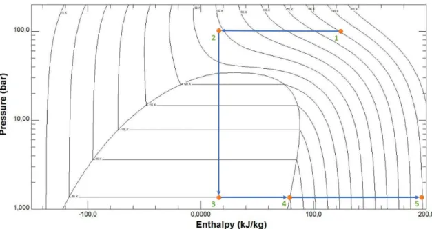
and is one of the requirements of ESA. When designing these type of systems, it is neces-sary to be aware of the processes that occur along the fluid path. These are represented in a PH diagram in figure 3.2and described in the text below.

• Point 1 to 2, The pressure is constant (≈100 bars), isobaric process; The fluid is

cooled by crossing the hot side of the heat exchanger that is in contact with the cold side.

• Point 2 to 3, the JT isenthalpic expansion takes place. The fluid is forced through the Joule-Thomson valve, it occurs a substantial temperature drop, and if T2is low

enough, part of the fluid passes to the liquid state.

• Point 3 to 4, the temperature (80 K) and pressure are constant and equal to the sat-uration pressure of nitrogen at 80 K (≈1.5 bar). This is where the heat is dissipated

by evaporation of the liquid nitrogen at constant temperature as far as the output pressure that is kept constant (let us remind that this pressure is mainly imposed by the adsorption cell).

• Point 4 to 5, the pressure is constant, isobaric process; The fluid temperature in-creases by exchanging the heat with the hot side of heat exchanger. In an ideal heat exchanger, and ifc_{p hot}> c_{p cold},T5reachesT1(180 K in our case)[6].

Table 3.1: System conditions

P1=P2= 100bar P3=P4=P5= 1.5bar

T1=T5= 180K T3=T4= 80K

H2=H3

The diagram of figure 3.2also allows to determinate the liquid fraction,x_liq:

xliq=

(H_liq−H3)

(H_gas−Hliq)

(3.1)

The Hliq is the liquid saturation enthalpy and Hgas the vapor saturation enthalpy,

equals toH4.

At 80 K the value obtained is,

(31)

Figure 3.2: Thermodynamic processes in a PH diagram. The various steps are explained in the text.

Knowing that a 1.5 W cooling power ( ˙Q) is needed, it is possible to estimate the gas flow required for the system.

˙

Q= ˙mL= ˙m(H4−H3) (3.2)

Lbeing the latent heat of vaporization. This results in the following nitrogen mass flow

˙

m= 23.7mg/s

It is very important to know this mass flow of nitrogen in the system before designing any component, because this it is essential for the components dimensioning.

3.2 Counterflow heat exchanger

The counterflow heat exchanger (figure 3.3) consists of two concentric tubes ("Tube-in-Tube" heat exchanger technique) with the function of transferring the heat of a fluid from a tube to another. The internal pipe is used for the high pressure to reduce the radial stresses due to its smaller diameter.

For the heat exchanger dimensioning, there are two major concerns:

(32)

• To ensure that, if possible, it behaves as an ideal heat exchanger, which means that all the heat that can be exchanged is exchanged along the heat exchanger. It can be achieved by increasing the length thus increasing the contact area between the two fluids.

a Schematic b Radius

Figure 3.3: Counterflow heat exchanger

3.2.1 Calculation of the pressure drop in HX tubes versus diameter

The most important parameter about choosing the diameter of the tubes is the pressure drop in the tubes ,∆_P, given by the expression below[6]

∆_P

L =fD

ρ

2

V2

D (3.3)

WherefD is the friction factor of the fluid. This factor is very sensitive to the fluid

regime (laminar or turbulent); in turbulent regime, it also depends on the roughness of the tube walls. Its variation with the Reynolds number, R_e, is depicted in the Moody diagram (figure 3.4).

(33)

The Reynolds number is the ratio between the inertial forces and viscous forces and, as show in figure 3.4 allows knowing the flow regime. It depends on the kinematic viscosity of the fluid, ν, the tube hydraulic diameter, D_h, and the mean velocity of the fluid,V:

Re Dh=

V Dh

ν (3.4)

The kinematic viscosity of the fluid, ν, is given by the ratio between the dynamic viscosity,µ, and density,ρ,

ν=µ

ρ (3.5)

And the mean velocity of the fluid, is given by the folowing expression:

V =V˙

A =

˙

m

ρA (3.6)

Being ˙V the volumetric flow rate andAthe cross section.

A=π

4Dh2 (3.7)

In our case, for a mass flow of 23.7 mg/s and at a temperature of 180 K (that is the worst case to ensure its working), applying these equations for both tubes, we calculate the Reynolds number as a function of the diameter (figure 3.5) in order to know the regime existing in the tubes. Note that for the low pressure tube, the hydraulic diameter is the diff_{erence between the tubes diameters.}

(34)

As demonstrated in figure 3.5: For high pressure, the fluid is clearly in laminar regime (Re lower than 2300) to the different diameters, due to the high density of the fluid. For

the lower pressure, to diameters lower than 1.2 mm, we are in the transition region to the turbulent regime but a priori these diameters are excluded, so it is also in laminar regime.

If the turbulent regime ( Rehigher than 4000) was reached, it would be necessary to

use the Colebrook–White equation to calculate thef_D but in our case, laminar flow,f_D is simpler and given by the following expression:

f_D =64

Re (3.8)

which leads us to the next simple analytical expression for the pressure drop,

∆_P

L = 128µ

˙

V

πD4 (3.9)

Using this expression, it is possible to trace the dependence of the pressure drop per meter as a function of the tube diameter hydraulic for high and low pressure (figure 3.6).

Figure 3.6: Curve of the evolution of pressure with diameter

(35)

3.2.2 Calculation of the tube thickness

It is now necessary to calculate the required thickness of the tubes to hold the pressure. In the case of capillaries, the name given to small diameter tubes, we can use the thin walls approach, applicable when the wall thickness is less than about a tenth of its radius[7].

In this case, it is only necessary to consider the radial stress and the following expres-sion allows to calculate the thickness.

σ=rP

t (3.10)

The thickness,t, is dependent on the yield strength of the material of the pipe walls,

σ, on his radius,r and on the subject pressure,P. To determine the thickness, it is only considered the high pressure side because it is the most critical, with a pressure of 100 bars. The wall material is composed by 304 stainless steel that has a yield strength of 250 MPa.

Using the approach for thin walls, we plot the thickness in function of the inner diameter of the high pressure tube (figure 3.7).

Figure 3.7: Thickness of the high pressure tube vs the inner diameter

As a precaution, it was set a thickness of 0.25mm because it is admissible for any diameter and it has a safety factor greater than 2.

In order to confirm the veracity of this approach there is the K factor, which is given by the ratio between the diameter and the thickness.

K=D

t (3.11)

(36)

Figure 3.8: Comparison of thin and thick cylinder theories for various diameter/thickness ratios[8]

3.2.3 Thermal exchange in the HX versus length

Knowing the diameters and the thickness of the tubes, the last geometrical parameter to take into account for effi_{ciency of the heat exchanger is its length. Applying the equations}

of heat balance at any point of the exchanger for an isolated system and using the notation defined in the figure 3.3a, temperaturesT2andT4are given by the equations[9],

(T1−T2) =η(T1−T3) (3.12)

(T4−T3) =W_W12

34η(T1−T3) (3.13)

being,

W = ˙mcp (3.14)

The efficiency of the exchanger,_η , which depends on the fluid, the diameter of the

inner tube (D) and the length (L) is given by:

η= 1−e−α

1−W_W12₃₄e−α

(3.15) α=       1

W12−

1 W34     

(37)

To help to understand the operation of the counterflow heat exchanger and the equa-tions it is represented in figure 3.9an example for the case wherecp hot> cp cold.

Figure 3.9: The temperatures profile inside the heat exchanger using notation of figure

3.3

In this last expression,h0is the overall heat transfer coefficient of the heat exchanger.

It depends on the heat transfer coefficient of the fluid in the hot and cold side,_h_in and

hout, on the conductivity of the material that separates the two tubes,k, and on the radius

of the heat exchanger tubes (figure 3.3b)[9]. It can be demonstrated

1

h0 =

r1out

h_inr1in

+r1out

k ln      

r1out

r1in

     + 1

h_out (3.17)

Finally it is necessary to calculate the heat transfer coefficient for fluids,_h_inand_h_out.

In the case of a forced convection inside tubes it can assume the following expression

h=Nuk

D (3.18)

Being the Nusselt number,Nu the ratio between the heat transferred by convection

and conduction:

NuL=_{Conductive heat transfer}Total heat transfer = hL_k (3.19)

In our case, as we are in laminar flow and we have an uniform surface heat flux for circular cross section tubes, the Nusselt number is constant[6],

Nu= 4.36 (3.20)

For technical reason, an outside diameter of 5.4 mm was the most appropriate for the low pressure tube. Using this value: the output temperature of the high-pressure pipe,

(38)

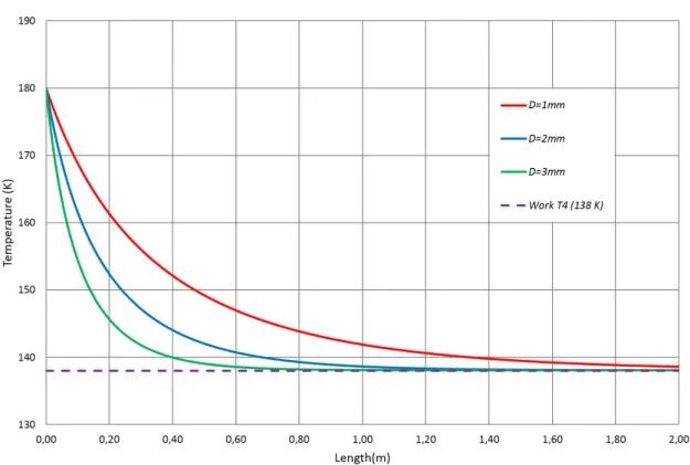
Figure 3.10: Plot of the output temperature of the high-pressure pipe with the length in the heat exchanger.

If we want to exclude HX longer than 2 meters, based on the plot we can exclude the diameter of 1 mm because it is not enough to cool the fluid to the desired temperature (138 K). In opposition the diameters of 2 mm and 3 mm are long enough to achieve the desired temperature.

Now, to choose between tubes it is necessary to confirm if the pressure drops are not significant. Remember that for the high pressure tube, the diameter had to be higher than 1 mm and for the low pressure tube, had to be higher than 2.8 mm.

Both diameters of the high pressure tube are higher than 1 mm, so we could chose any one. However, when we calculate their hydraulic diameters, not forgeting of adding their thickness, to the low pressure tube, we obtain an hydraulic diameter of 2.9 mm with the tube of 2 mm and 1.9 mm for the of 3 mm. Therefore, the tube of 3 mm is excluded and the chosen one is the tube of 2 mm.

With the chosen diameters we can plot the temperature profile along the length of the heat exchanger tubes (T2andT4) to define the length of heat exchanger. Those

tem-peratures are represented in the next graph (figure 3.11). From this plot (figure 3.11), it can be seen that in exchangers with a length,L, longer than≈1.5 m,T2andT4do not

(39)

Also, it is important to note that the fact that there is a larger temperature variation on the cold side in relation to the hot side that allows theT4temperature to be equal to

T1is due to the fact that the heat capacity of nitrogen at a constant pressure of 100 bars

is higher than at 1 bar.

Figure 3.11: Plot of temperature evolution with the length of the heat exchanger

To sum up the heat exchanger dimensions are displayed in table 3.2. Table 3.2: Heat exchanger dimensions

D1in 2 mm

D1out 2.5 mm

D2in 5.4 mm

D2out 6 mm

(40)

3.3 Joule-Thomson valve

A Joule-Thomson valve expansion consists on forcing the gas to pass through a restriction, small enough to cause a significant pressure drop (isenthalpic expansion).

The way of characterizing the Joule-Thomson valve effect is through the Joule-Thomson

coefficient,

µ_JT =

      ∂T ∂P       H (3.21)

The Joule-Thomson coeffi_{cient indicates if the temperature increases or decreases}

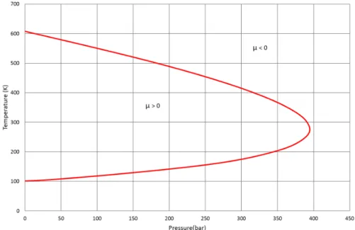
after an expansion (dP <0). From equation 3.21, we can see that the fluid inversion temperature corresponds to the temperatures for which this coeffi_{cient is equal to zero}

and the fluid cools only ifT_in< T_inv. The red curve limits the zone where the temperature decreases after the expansion to a certain pressure (figure 3.12).

Figure 3.12: Graph of nitrogen inversion curve on the Joule-Thomson limits the zone of decreasing temperature

The valves that we tested were basically constituted by a gland with a hole in its center, this hole was made with a laser beam. The diameter of this hole must ensure the target mass flow of nitrogen at the pressure and temperature wanted.

When a compressible flow finds a restriction, by the principle of mass conservation, the velocity needs to increase to cross the restriction (figure 3.13). The fluid speeds up until it reaches the sound velocity of this fluid under such conditions of pressure and temperature. This eff_{ect is called choked flow, the velocity of the fluid becomes choked or}

(41)

Figure 3.13: Schematic of the Joule-Thomson valve

In choked conditions and assuming an ideal gas behaviour, the equation for the mass flow rate in SI units is:

˙

m=CdA

v u u t kρP       2

k+ 1

      k+1

k−1

(3.22)

Being Cd the discharge coefficient (ratio of the actual discharge to the theoretical

discharge),Athe restriction cross-sectional area, kthe heat capacity ratio (C_p/C_v),ρthe density before expansion andPthe upstream pressure.

Actually, the problem is not simple. For instance, in our working conditions (100 bar and 138 K), the fluid can not be considered an ideal gas. To overcome this problem we have two main ways: one is to use real gas property data, like those given by REFPROP program [11], and the discrepancy in respect to these results incorporated in aC_d;

The other way is to use the correlations from a model developed by Maytal et al., also to ideal gas[12]. So, considering the density of an ideal gas,

ρ= P

T R_s (3.23)

BeingR_sthe specific gas constante (in case of nitrogenR_s= 296.8J/kg.K), it is possible to rewrite the mass flow expression for an ideal gas.

˙

mideal=CdAP

v u u t

k

T Rs

      2

k+ 1

      k+1

k−1

(3.24)

In the Maytal’s model, the isentropic and isenthaplic conservation law through the process is solved considering that the flow velocity at the end of the expansion is equal to the sound velocity. Considering the law of the corresponding state, a correlation factor,Γ_{, is obtained as a function of the reduced pressure (}Π₀₌_P/P_c_{), and temperature}

(42)

Figure 3.14: The Maytal correlation factor[12]

Then for real gases it is applied the correlation factor (Γ₎

˙

m=Γ_m˙_ideal (3.25)

(43)

C

h

a

p

t

e

r

4 E x p e r i m e n ta l Se t u p

During the course of the thesis, it was decided to test the Joule-Thomson (JT) valve sep-arately of the counterflow heat exchanger. This decision was driven by the necessity to characterize the JT orifices in real conditions of pressure and temperature, independently of the performances on counterflow heat exchanger. Such strategy would theoretically help to detect the cause of an eventual dysfunction of the cold part.

4.1 Experimental setup for the Joule-Thomson valve

To characterize the JT valve it was necessary the to design a system capable to create the real conditions (Tin andPin) at the input of the JT restriction. This system was divided in

two parts: one responsible for the pressure and mass flow (gas bottle, pressure regulator and manifold) and other for the temperatures (Cold finger). The schematic of the system used is represented in figure 4.1.

(44)

C H A P T E R 4 . E X P E R I M E N TA L S E T U P

In this early stage of this project, the sorption compressor, responsible for providing a gas flow, was still under study and was substituted by a pressurized gas bottle equipped with a pressure regulator. This gas bottle ( "B50" cylinder) provides and maintains the necessary gas flow to the system and then the gas is released to atmosphere by a home-made one way valve. Actually, this system was very functionnal for the tests performed during this work due to its low costs and simplicity.

The valve panel (manifold) built is showed in figure 4.2as well as the gas bottle and pressure regulator. Let us note that this panel was designed by Jorge Barreto in order to incorporate others funcionalities allowing to work with neon in the next future. This panel has the function of managing the course of the fluid and to measure the pressure and mass flow.

Figure 4.2: Gas control system assembly

To provide the right temperature (138 K) at the input of the JT valve was not so easy, to do this it was necessary to use a cryocooler already existing in the Cryogenic lab. The cryocooler was adapted like demonstrated in the next figure 4.3.

(45)

Figure 4.3: Schematic of the Joule-Thomson system

The first exchanger is thermalized in the first stage of the cryoccoler (T= 26 K, not controllable) and is responsible for precooling the gas from room temperature down to around 160 K. The final precooling down to the desired temperature (138K) is ensured by the second heat exchanger thermalized in the second stage (Cold finger). As a matter of fact, this second stage is equipped with a heater (H2) that allows to control its temperature so we attached the second heat exchanger directly to this stage and in this way we can control the diff_{erent temperatures of the test by changing the temperature of the second}

stage.

But for this to work it was necessary to calculate the correct dimensions of the heat exchangers that enable to simulate normal work conditions, 100 bar and 138 K at the entrance of the Joule-Thomson valve with a mass flow of 23.7 mg/s.

Using the same type of calculation that was used in section 3.2.3, it is obtained the following expression for the length [9]:

(T0−T2) = (T0−T1)e−

πhDL

˙

mcp _(4.1)

beingT0the temperature of the copper block,T1 the temperature of the fluid at the

heat exchanger inlet andT2the outlet.

(46)

the next plot (figure 4.4), where we can see that after 65 mm the temperature of the gas temperature decreased from room temperature down to 160 K which is low enough to allow a second heat exchanger relatively short do the rest.

Figure 4.4: Plot of the evolution of the temperatures with the length in HX1

Again using the previous expression for HX2 we can calculate the evolution of the temperatures with the length of the heat exchanger. In figure 4.5, it can be seen that using a temperature of 50 K in the second stage and 20 mm long heat exchanger it is possible to achieve temperatures around 138 K, that is the same temperature that we want to achieve at the outlet of the conyterflow HX (see section 3.1).

(47)

Actually, we faced the following technical problem: if we connect the first heat ex-changer directly in the first stage, it will cool down to a temperature between 25-30K, equilibrium temperature of this stage, not controllable, then, at the beginning of an ex-periment, when the nitrogen starts to circulate, it solidifies (Tsol≈63K), clogging the tube

along this HX without any solution to restore the nitrogen flow. To solve this problem, we limited the power exchanged between the HX1 and the first stage by using a copper link and installing a heater resistor, H1, (300 Ohms) on the HX1 copper block . The copper link allows cooling the heat exchanger but also to warm it with a reasonable heating power when necessary.

To dimension this copper link, taking into account that it must allow a gas cooling down to at least 160 K in the stationary regime (constant mass flow), we considered that the cooling power at 160 K needed to cool the gas from room temperature (equation4.2) is provided by this heat link (equation4.3), with∆_T = (160_K₋25_K) and a mass flow a

little higher, around 35 mg/s in order to consider a possible higher mass flow that could occur due to uncertainty in the JT performances.

˙

Q= ˙m(H300K,100bar−H160K,100bar) (4.2)

˙

Q=−kS

L∆T (4.3)

This calculation indicates that 6 wires of copper (RRR= 100), with 60 mm long and 1 mm of diameter, mounted in parallel would be a good solution.

(48)

4.1.1 Manufacturing of the Joule-Thomson system

The first heat exchanger (HX1)

The first heat exchanger consists on a tube (65 mm long and 1.5 mm inner diameter) wrapped around a copper cylinder with a diameter of 12 mm. Being this diameter rel-atively small, we had to prevent some tube crushing during this winding: the tube was first filled with liquid water, freezed, and then wound around the copper cylinder. After the shaping phase, the tube was then welded with a soft solder (Sn96.3%Ag3.7%) with a

melting point of 221◦_C _(figure _4.6a_).

The copper link was made using 6 wires welded to a plate of copper. After that the HX1 was assembled in the cryocooler as shown in figure 4.6b.

a HX1 b HX1 coupled to 30 K stage

Figure 4.6: The first heat exchanger (HX1)

The second heat exchanger (HX2)

(49)

a HX2 b HX2 assembled on cold finger stage

Figure 4.7: The second heat exchanger (HX2)

Joule-Thomson valve

The Joule-Thomson valve was manufactured from a Swagelok©VCR Blind Gland of 1/4 inch. First, the Gland was drilled with a diameter of 4.75 mm to obtain a thickness of 2.54 mm and then using a laser it was made the restriction (see in Appendix A.1.2). Being the manufacturing uncertainty of 10 %, the diameters was measured using a Scanning electron microscope, SEM, (Figure 4.8). For the orifices used in this work, diameter of 25.05µmand 49.25µmwere mesured for nominal diameters of 25µmand 45µm.

(50)

We decided to make the Joule-Thomson valve in a Blind Gland to change it more easily. To insert the gland in the gas circuit we had to manufacture others pieces to connect with the tubes, welded by the normal method.

To finish we placed the heaters and the thermometers. For both the method used was the same, a copper foil was welded directly on the tube and the heaters or thermometers were connected on the foil. All this is demonstrated on figure 4.9and 4.10.

(51)

(52)

4.1.2 Control and Acquisition System

The control and acquisition system uses several devices, some are indicated in figure 4.11

and others, like the Flowmeter, were already mentioned at the beginning of this chapter. The functions of the devices are described in table 4.1.

Figure 4.11: Control and Acquisition devices

Table 4.1: Functions of the control and acquisition devices

Device Function

Cryocontemperature Measures several temperatures (T1, T2, T7) and

controller (model 24 C) controls the temperature of HX1

Cryocontemperature Measures several temperatures (T3, T4, T5, T6) and

controller (model 34) controls the cold stage 2 of the cryocooler

AgilentDC Power Controls the Power applied (H3)

Source (model E3631A) in evaporator

AgilentDigital Multimeter Measures the pressures by converting

(model 34402A) the analog signal of the pressure sensor Computer Communication between the

LabV IEWT Mand the devices

The interface between the devices and the user was adapted from a priorLabV IEWT M

(53)

The figure 4.12displays the main interface of theLabV IEWT Mprogramm. Various others "tabs" allow the monitoring of others parameters with special details.

Figure 4.12: Main tab of theLabV IEWT Mprogram. This tab monitors the temperature, pressure and flow rate through the system.

4.1.3 Mechanical tests

Before any test, all the pieces of the systems had to be cleaned and validated. To clean the pieces, a system made with a water pump and an ultrasound bath was mounted. The water pump was used to force the circulation of isopropyl alcohol inside the pieces, removing dirt and grease and also to make sure that nothing was clogged. Meanwhile, the piece was dipped in an ultrasound machine at 40◦_C_{to increase the e}ffi_{ciency of the}

cleaning process.

When required, after cleaning, all the pieces were subject to leak test with a INFI-CON®(model: UL1000) helium leak detector. The tests were made in vacuum mode or/and by "sniff_{er mode", this one allows to put the various tubes under pressure, namely}

closer of the real conditions. All of the pieces must had a gas leak inferior to ≈ 10−7

mbar.L/s.

(54)

4.2 Experimental setup for the Cold part

Without the correct Joule-Thomson restriction we could not test the entire cold stage and consequently the counterflow heat exchanger, because we do not have the right mass flow in the right conditions. It was decided that in first place we would project the cold stage in SOLIDWORKS without the JT valve. Because the entire low temperature part will be tested in a small cryocooler (2W@ 20K) available in the Cryogenics lab, it was necessary to take into account the dimmensions already defined by this cryocooler. And this way, we could ensure that everything fits before assembling and also helped the dimensioning of others pieces. The result is showed in figure 4.13.

(55)

The test system in this the cryocooler was made in a similiar way to that was described in section 4.1.1. However, being this cryocooler smaller, the compactness of the several elements were optimized. Moreover, as far as possible, the various circuit sections are made to be detachable. Then, after all set in the drawing we start building the cold part without a JT valve.

Counterflow heat exchanger

As explained in section 3.2.3the heat exchanger has a length of 2 m with two tubes, one inside the other (dimensions in table 3.2), in order to turn the heat exchanger more compact these two meters were wounded on a diameter of 60 mm. Similarly to the HX1 manufacturer, to avoid tube crushing, we fill the low pressure tube with salt, instead of water and due to the long length a wire was introduced in the 6 mm tube (low pressure tube) to be used as a guide to allow pulling the high pressure tube through the low pressure one after winding. The winding process is showed in (Figure 4.14).

Figure 4.14: The counterflow Heat Exchanger during the winding process

(56)

Figure 4.15: The counterflow Heat Exchanger

(57)

The final result is shown in figure 4.17.

a Projected b Manufactured

(58)

(59)

C

h

a

p

t

e

r

5

R e s u lt s a n d d i s c u s s i o n

5.1 Joule-Thomson valve

5.1.1 Mass flow

The first characterization made with Joule-Thomson valve was the determination at room temperature (T = 300 K) of its discharge coefficient, _C_d (see in section 4.1). So, we

measured the flow under diff_{erent inlet pressures for both restrictions (49.25} _µ_{m and}

25.05µm). The results are displayed in the next plots, the figure 5.1represents the mea-sured flows and figure 5.2the discharge coefficients, both calculated using the equation 3.22and REFPROP data.

(60)

C H A P T E R 5 . R E S U LT S A N D D I S C U S S I O N

Through the results we can conclude that on 49.25µm the mass flow is too high (45 mg/s at 100 bar) and too far from the desired 23.7 mg/s at 100 bar. Also on the 25µm, the mass flow will be probably too high because the mass flow obtained (13 mg/s) is already near to the objective at room tempetaure, and the decreasing of the temperature to the work temperature will cause an increase of density and a consequently an increase of the mass flow.

Figure 5.2: The discharge coeffi_{cients in function of pressure at room temperature for}

both restrictions using equation 3.22and REFPROP data and the dashed lines represents its average value

The figure 5.2seems to show that theCdslightly increases with the pressure. However,

by a simpler way, it was obtained an average Cd of 85% for the restriction of 25.05µm and an averageCd of 89% for the restriction of 49.25µm. Then, we started testing the

theoretical equations at lowest temperatures, in order to know if these equations allow us to find the correct orifice diameter for the target mass flow of 23.7 mg/s at 100 bar and 138 K.

(61)

Figure 5.3: Interface of theLabV IEWT Mduring a test system at 38.2 bar and a mass flow of 502 mL/min. Note the stable temperature of 140.86 K achieved before the expansion (violet line)

So, with the system working it was tested the restriction of 49.25µm at a fixed pressure of 50 bar and decreasing the inlet Temperature 300 K to 140 K (Figure 5.4) and repeated for the restriction of 25.05µm at 60 bar (Figure 5.5). In these figures, the experimental results (blue line) are compared to the equation 3.22with REFPROP data (red line) but also the equation 3.24for ideal gas (yellow line) and Maytal[12], equation 3.25(green line).

(62)

Figure 5.5: The mass flow in function of temperature at a pressure of 60 bar to the restriction of 25.05µm with aCd of 85%

In general, the flow increases as T decreases, mainly due to the increase of density. In the plot 5.4we can observe that when we start decreasing the temperature, the devia-tions between the theoretical curves and experimental ones increase and the discharge coeffi_{cient can no longer correct that di}ff_{erences between them.}

It also should be noted that we are with a mass flow much higher than the desired and only in half of the desired pressure. And the flowmeter also has a limitation on the mass flow of around 40 mg/s, so considering this data, we decided to discard this restriction and to work only with the restriction of 25µm. On the plot of figure 5.5we had basically the same type of results: discrepancy increase with T and despite the flow being significantly reduced, it is too high in what reff_{ers to our requirements.}

But since this orifice was the smallest available at that time, we decided to characterize only this restriction in order to obtain correlations and to compare them with those pro-posed by Maytal. Then from those correlation obtained, we could dimension the needed diameter of the next restriction with some reliability. So, to optimize time and compare with the Maytal’s results, we made the measurements at a constant temperature as a func-tion of pressure and the experimental results are displayed in figure 5.6(T_in = 151K) and 5.7(Tin = 141K).

The correlations of factor gamma,Γ_{, are obtained dividing the experimental results}

obtain for the mass flow by the calculations for the mass flow in a ideal gas. These results are replotted as a function of Π₀(_P/P_c_{, P}_c= 34_bar) and for the two diff_erentΘ₀

(63)

Figure 5.6: The mass flow in function of pressure at a temperature of 151 K to the restriction of 25.05µm with aC_d of 85%

(64)

Figure 5.8: Comparison of the Maytal’s correction factor Gamma[12] and our results. Black lines: Maytal’s results, red line: 151 K; blue line: 141 K, yellow point: extrapolated and green point Maytal’s result both under our work conditions

Once again the flows were already too high at 90 bar and 141 K, very close to the highest detection limit of the flow meter. That is why we could not get closer of the work conditions but in order to determine the appropriate diameter for the orifice using the equation 3.25, we had to obtain the gamma factor to ours work conditions from the previous curves. So, to do that we had to extrapolate a gamma for these conditions,

Π₀= 2_.94 andΘ₀= 1_.10,

Γ∗_{= 2}_.₉₃ _(5.1)

and under our work conditions by Maytal’s correlation:

Γ= 2_.15 (5.2)

So we used both correlations to have an idea of the restrictions diameter. The results are indicated in table 5.1.

Table 5.1: The predicted diameters for a flow of 23.7 mg/s

Γ Diameter (_µm)

Γ_{= 2}_.₁₅ _{18.2 (}_C_d_{= 100%)} _{19.5 (}_C_d_{= 87%)} Γ∗_{= 2}_.₉₃ _{15.6 (}_C

(65)

5.1.2 Thermodynamic of the cold part

Despite of the fact that the target flow conditions were not obtained with the smallest orifice, we tested if, in the available conditions of temperature and pressure with the 25 microns orifice, the results obtained after the JT expansion were in agreement with those expected from thermodynamics.

To test the isenthalpic expansion in the Joule-Thomson valve we used the case with a fixed pressure of 60 bar for five diff_erent_T_in _(Figure _5.5_{). These are represented on the}

PH diagram (Figure 5.9) and the results are demonstrated in table 5.2.

Figure 5.9: Representation of the isenthalpic expansion in the Joule-Thomson valve at 60 bar.

Table 5.2: Results of the isenthalpic expansion at 60 bar. Tin, TJT andTevap correspond

respectively toT4, T5andT6in figure 4.3. Texpexted is obtained from the PH diagram of

figure 5.9

n◦ _m˙₍_mg/s₎ _T

in(K) TJT(K) Tevap(K) Texpected(K)

1 12 170 153 130 129

2 14 160 146 112 111

3 19 150 140 90 89

4 26 144 135 77.5 77.8

5 27 142 132 77.4 77.8

(66)

A second test consists on checking if the cooling power is in agreement with our calculations.

To calculate the cooling power that we are capable of producing we need to be on a situation where we are producing liquid nitrogen on the evaporator. Then the cooling power corresponds to the heating power needed to evaporate exactly the liquid quantity formed after the JT expansion.

For example if we choose the point 5 of the table 5.2, a quite high power has to be applied in order to make sure that we are evaporating all the liquid and then start decreasing this power until we get a balance between the liquid nitrogen that is formed and the evaporated.

A way to see this process is through the temperatures (Figure 5.10), when we apply a power higher than a cooling power we also are increasing the temperature of thermome-ters nearby, like T_out. Therefore, when the T_out is equal toT_evap means that we are in the balance. It is clear that if we continue to decrease the power, the temperatures will remain the same because we are accumulating liquid, that is why we need to start in a higher power applied. The temperature versus the applied power as plotted in figure (Figure 5.11).

(67)

Figure 5.11: Dependence ofTout and heating power applied (H3) during the process of

cooling power (CP) determination.

As demonstrated we obtained a cold power of around 500 mW. The theoretical cold power corresponding to this thermodynamic process can be calculated using the equation

3.2,

˙

Q= 27×10−3(H60bar,142K −H1bar,78K)≈500mW (5.3)

(68)

(69)

C

h

a

p

t

e

r

6

C o n c l u s i o n s

This thesis had as main objective the construction and characterization of the cold part of a 80 K vibration-free cooler.

Due to technical and temporal reasons, this main objective was splitted in two. Both were essential, one of them was the characterization of the Joule-Thomson restrictions and the construction of the respective test system, capable of precooling the flow down to the required temperature (138K); the other objective was the dimensioning of the counterflow Heat Exchanger and its construction.

The system to precool the flow was mounted in a already existing cryocooler and it was a success: we were able of setting a desired temperature at the entrance of the Joule-Thomson valve with high accuracy. This system allowed us to obtain the flow to characterize the restrictions for several temperatures and pressures.

The results showed that our restrictions were too large since the mass flows obtained exceeded the target conditions: the 25 mg/s flow was obtained at 142 K with a pressure of 60 bar instead of 100 bars using the restriction with a diameter of 25 µm. We also found out that there is a significant difference between the results and the expected mass

flows for ideal gases, using REFPROP data and Maytal’s correlations. This diff_erence

increases as the inlet temperature decreases and not even with the Maytal’s model we could reproduce our results. This error could be due to the irregularity of the restriction geometry made by the laser, as demonstrated in SEM pictures. If that is the case, the right orifice, leading to the target conditions, will be obtained by try and error. However, now with the correlation obtained, we can extrapolate some possible diameters for the orifice (Table 5.1). So, for our mass flow we need a diameter around 17µm. The new orifices were ordered recently and will be tested in the near future.