2016 | Lavras | Editora UFLA | www.editora.ufla.br | www.scielo.br/cagro
http://dx.doi.org/10.1590/1413-70542016405011416
Mapping soils in two watersheds using legacy data and extrapolation
for similar surrounding areas
Mapeamento de solos em duas sub-bacias hidrográficas usando dados legados e sua
extrapolação para áreas similares do entorno
Marcelo Henrique Procópio Pelegrino1, Sérgio Henrique Godinho Silva2*, Michele Duarte de Menezes1,
Elidiane da Silva1, Phillip Ray Owens3, Nilton Curi1
1Universidade Federal de Lavras/UFLA, Departamento de Ciência do Solo/DCS, Lavras, MG, Brasil 2Universidade Federal dos Vales do Jequitinhonha e Mucuri, Instituto de Ciências Agrárias, Unaí, MG, Brasil 3Purdue University, Department of Agronomy, West Lafayette, Indiana, United States
*Corresponding author: sergiohgsilva@gmail.com Received in March 18, 2016 and approved in May 2, 2016
ABSTRACT
Existing soil maps (legacy data) associated with digital mapping techniques are alternatives to obtain information at lower costs, however, tests are required to do it more efficiently. This study had as objectives to compare different methods to extract information from detailed scale soil maps using decision trees for mapping soil classes at two watersheds in Minas Gerais, validate these maps in the field and use the best method to extrapolate information to larger areas, also validating these maps of larger areas. Detailed soil maps of Vista Bela creek (VBW) and Marcela creek (MCW) watersheds were used as source of information. Seven methods to extract information from maps were compared: the whole polygon, eliminating 20 and 40 m from the polygon boundaries, and with buffers around the sampled points with radii of 25 m, 50 m, 75 m, and 100 m. The Classification and Regression Trees (CART) algorithm was employed to create decision trees and enable creation of soil maps. Accuracy was assessed through overall accuracy and kappa index. The best method was used to extrapolate information to larger areas and maps were validated. The best methods for VCW and MCW were, respectively, eliminating 20 m from polygon edges and buffer of 25 m of radii from points. Maps for larger areas were obtained using these methods. Removing uncertainty areas from legacy soil maps contribute to better modeling and prediction of soil classes. Information generated in this work allowed for validated extrapolation of soil maps for regions surrounding the watersheds.
Index terms: Decision trees; pedology; tropical soils.
RESUMO
Mapas de solos existentes (dados legados) associados a técnicas de mapeamento digital são alternativas para obter informações a menores custos, entretanto, alguns testes são necessários para se fazer isso de forma mais eficiente. Este estudo objetivou comparar diferentes métodos para extrair informações de mapas de solos em escala detalhada usando árvores de decisão para mapear classes de solos em duas sub-bacias hidrográficas de Minas Gerais, validar os mapas em campo e usar o melhor método para extrapolar informações para áreas maiores, também validando estes mapas. Mapas de solos detalhados das sub-bacias do ribeirão Vista Bela (VBW) e ribeirão Marcela (MCW) foram utilizados como fonte de informação. Sete métodos para extrair informações de mapas foram comparados: polígono todo, eliminando 20 e 40 m das bordas dos polígonos, e com buffers em torno dos pontos amostrados com raios de 25 m, 50 m, 75 m e 100 m. O algoritmo Classification and Regression Trees (CART) foi utilizado para gerar árvores de decisão e permitir a criação de mapas de solos. A acurácia dos mapas foi avaliada através da acurácia global e índice Kappa. O melhor método foi utilizado para extrapolar informações para áreas maiores e esses mapas foram validados. Os melhores métodos para VCW e MCW foram, respectivamente, eliminando 20 m das bordas dos polígonos e buffer com raio de 25 m ao redor dos pontos. Mapas para áreas maiores foram obtidos usando esses métodos. Remoção de áreas de incerteza de mapas legados de solos contribuem para uma melhor modelagem e predição de classes de solos. A utilização de informações geradas neste trabalho permitiu a extrapolação validada de mapas de solos para regiões do entorno das sub-bacias hidrográficas.
Termos para indexação: Árvores de decisão; pedologia; solos tropicais.
INTRODUCTION
Soil survey reports and maps are very important for use and sustainable management of soils, making it possible to obtain the most of their productive potential, urban planning and the final destination of waste (Resende et al., 2014). However, in Brazil,
financial resources for soil surveys are scarce, and most existing detailed maps are common only for small areas,
which were usually created to serve specific projects
surveys in a more detailed scale, an alternative is the use of pre-existing information (Bui and Moran, 2001), so called soil legacy data.
Soil legacy data, including maps with legends, reports, morphological descriptions and analyses of
modal profiles and extra-samples, can be used to recover
the pedologist’s mental model on the distribution of soils on the landscape (Bui, 2004). However, in Brazil, most of the soils information is included in conventional analogic maps, published at small scales, from which the pedologist’s mental model is not easily obtained and understood, since the mapping units are less homogeneous than those present in more detailed soil
maps. This fact tends to make the refinement of these existing maps more difficult.
As an alternative to the improvement of the scales of soil maps, in recent years an increasing number of digital soil mapping tools has been created, aiming to establish statistical and mathematical relationships between environmental covariates and soil classes and properties to be predicted and spatialized (Giasson et al., 2015). In this sense, soil legacy data can be explored by new techniques, such as data mining, allowing for recovery of soils information for further prediction and spatialization.
Among the available tools for data mining are decision tress. They have as main advantages the ease of interpretation and discussion, relative simplicity in modeling not additive and non-linear relationships, the ability to deal with both categorical and numerical data (Greve et al., 2010), besides the process of acquiring information being relatively quick. Decision trees can also help in the choice of terrain attributes that can constitute the best predictors for soil classes and properties. This data mining technique was used by Caten, Dalmolin and Ruiz (2012), Scull, Franklin and Chadwick (2005), Zhou, Zhang and Wang (2004), helping understand the distribution of soils on the landscape.
However, as well as most techniques, decision trees also have some limitations, such as the possibility of the employed algorithm to choose variables that have more distinct values to be used as splitters if everything else is kept the same, which may affect the integrity of inferences made based on decision trees (Loh, 2011). In addition, when used to recover soil map information, if soils are represented in less homogeneous pedological mapping units or if soils occur in an intricate pattern on the landscape, this may limit the decision trees ability to make correct predictions (Silva et al., 2016).
In this sense, a possibility to solve these constraints may be to extract soils information only from parts of detailed soil maps on which the pedologists who created the map were more precise about the presence of soil classes, such as the central parts of the polygons, since polygon borders are considered transitional zones between soil classes, and around the sampling
points, places where a formal soil classification was
performed. Thus, those places may adequately represent environmental conditions of a soil class to occur and, for this reason, to study them may be an alternative to
improve the efficiency of decision trees to model and
predict soil classes and properties. Caten, Dalmolin and Ruiz (2012) and Giasson et al. (2015) used semi-detailed soil maps to obtain information for training decision trees to map soil classes, avoiding samples at different distances from map unit boundaries. However, the use of a detailed soil map as source of data, the comparison between information collected avoiding polygon boundaries with information obtained within
varying distances from sampling points, where profile
descriptions were performed, culminating with the use of the best generated models to extrapolate information to map soils of areas with similar environmental conditions, assessing their accuracy, may constitute alternatives to improve existing soil maps.
In this context, this study aimed to: (i) compare different methods to extract information from detailed scale existing soil maps, using decision trees, for mapping soil classes in two watersheds in Minas Gerais,
validate the maps in the field to assess the influence of
sites in recovering the pedologist’s mental model; and (ii) use the best method as a basis for extrapolation of soils information to similar areas surrounding these watersheds, and validate the generated maps of larger areas.
MATERIAL AND METHODS
Study areas
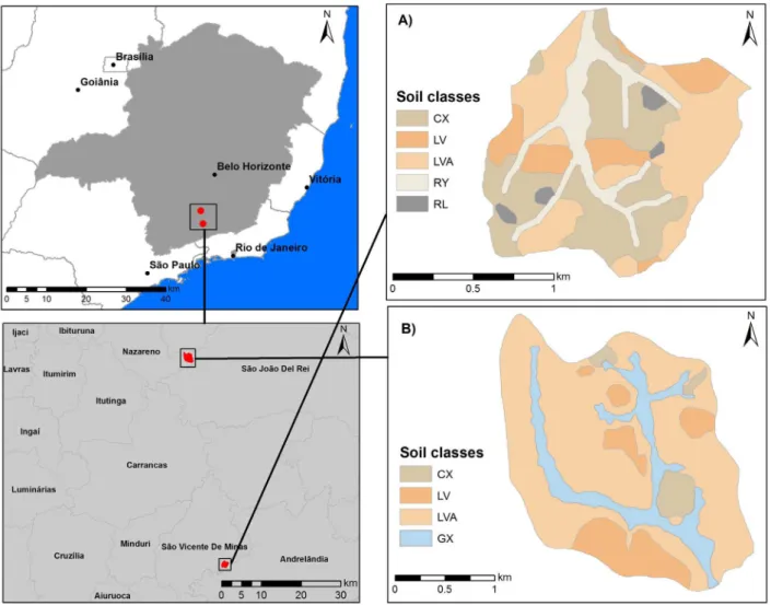
This study was conducted in two watersheds of Minas Gerais, named Vista Bela Creek watershed (VBW) and Marcela Creek Watershed (MCW) (Figure 1). The VBW is located on the right bank of the Aiuruoca river, in the Andrelândia county. It is located between the latitudes 7597109 and 7598777 m and longitudes 559895 m and 561563 m, zone 23K, datum Córrego Alegre, with an area of 175 ha. It has Cwa climate,
and rainy summers. Altitude ranges between 960 and 1080 m and it is occupied by Haplic Cambisols (CX - 35.1%, Ochrepts), Red-Yellow Latosols (LVA - 34.9%, Orthoxes), Fluvic Neosols (RY - 15.6%, Fluvents), Red Latosols (LV - 12.1%, Orthoxes), and Litholic Neosols (RL - 2.3%, Orthents), with gneisses and biotite-schist as parent materials (Menezes et al., 2009).
The MCW is a tributary on the right bank of
Jaguara creek that directly flows into the Hydroelectrical
power plant reservoir of Itutinga-Camargos/CEMIG. It is located between the longitudes 550169 and 552810 m and latitudes 7650163 and 7650989 m, zone 23k, datum Córrego Alegre, in Nazareno county, and it has
485 ha of area. The climate is Cwa, according to Köppen
classification, and altitude ranges from 960 to 1060 m.
The occurring soils are Red-Yellow Latosols (LVA - 65%, Orthoxes), Red Latosols (LV - 14%, Orthoxes), Haplic Gleysols (GX - 17%, Acquents) and Haplic Cambisols (CX - 5%, Ochrepts). MCW has as parent material the product of altered mica schists of the Andrelândia Group, Upper Proterozoic (Motta et al., 2001). Soil legacy data used as a source of information for this study were detailed scale soil maps resulted from conventional pedological surveys, published at scales of 1:10,000 in VBW (Menezes et al., 2009) and 1:12,500 in MCW (Motta et al., 2001) (Figure 1).
Digital soil mapping using decision trees
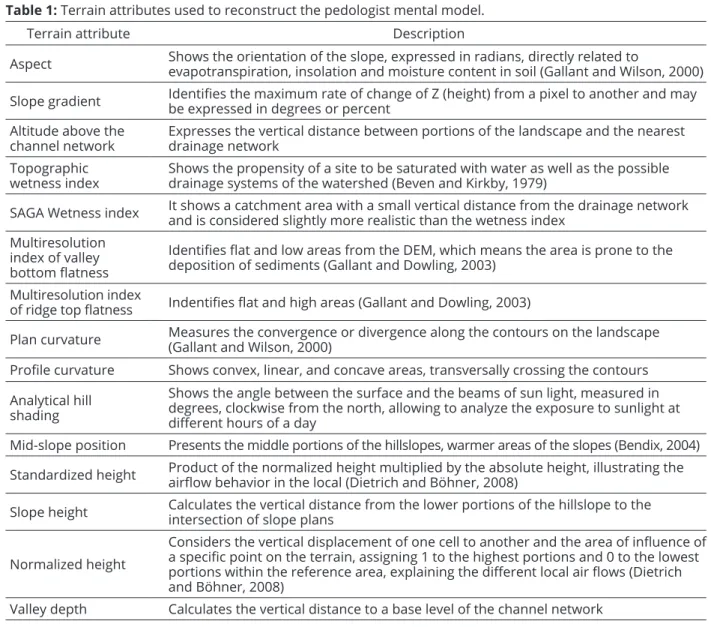
Digital Elevation Models (DEM) with a spatial resolution of 10 m were generated for each watershed from contour lines at 1:50,000 scale (IBGE), in ArcGIS 10.1 software (ESRI) through the Topo To Raster tool. From the DEM, 15 terrain attributes (TA) were generated for each watershed (Table 1), including: aspect, slope, altitude above the channel network, topographic wetness index, SAGA wetness index, multiresolution index of
valley bottom flatness (MRVBF), multiresolution index of ridge top flatness (MRRTF), plan and profile curvatures,
analytical hill shading, mid-slope position, standardized height, slope height, normalized height, and valley depth.
SAGA GIS, version 2.1.4 (Böhner, McCloy and Strobl, 2006) and ArcGIS 10.1 were used in this procedure.
The methods to extract information from soil maps considered polygons of mapping units and the sampling points. Therefore, the 15 terrain attributes were overlaid on soil maps and the pixel values were related to the corresponding soil class. Two extraction methods were evaluated in order to compose the database and to create decision trees:
1) Polygons of mapping units (PM): a) the entire polygon, b) interior of the polygon eliminating 20 m from its boundaries; and c) interior of the polygon eliminating 40 m from its boundaries (Figure 2A). Those distances were chosen in order to avoid that smaller mapping unit
Table 1: Terrain attributes used to reconstruct the pedologist mental model.
Terrain attribute Description
Aspect Shows the orientation of the slope, expressed in radians, directly related to evapotranspiration, insolation and moisture content in soil (Gallant and Wilson, 2000)
Slope gradient Identifies the maximum rate of change of Z (height) from a pixel to another and may be expressed in degrees or percent
Altitude above the channel network
Expresses the vertical distance between portions of the landscape and the nearest drainage network
Topographic wetness index
Shows the propensity of a site to be saturated with water as well as the possible drainage systems of the watershed (Beven and Kirkby, 1979)
SAGA Wetness index It shows a catchment area with a small vertical distance from the drainage network and is considered slightly more realistic than the wetness index
Multiresolution index of valley bottom flatness
Identifies flat and low areas from the DEM, which means the area is prone to the deposition of sediments (Gallant and Dowling, 2003)
Multiresolution index
of ridge top flatness Indentifies flat and high areas (Gallant and Dowling, 2003)
Plan curvature Measures the convergence or divergence along the contours on the landscape (Gallant and Wilson, 2000)
Profile curvature Shows convex, linear, and concave areas, transversally crossing the contours
Analytical hill shading
Shows the angle between the surface and the beams of sun light, measured in degrees, clockwise from the north, allowing to analyze the exposure to sunlight at different hours of a day
Mid-slope position Presents the middle portions of the hillslopes, warmer areas of the slopes (Bendix, 2004)
Standardized height Product of the normalized height multiplied by the absolute height, illustrating the airflow behavior in the local (Dietrich and Böhner, 2008)
Slope height Calculates the vertical distance from the lower portions of the hillslope to the intersection of slope plans
Normalized height
Considers the vertical displacement of one cell to another and the area of influence of a specific point on the terrain, assigning 1 to the highest portions and 0 to the lowest portions within the reference area, explaining the different local air flows (Dietrich and Böhner, 2008)
polygons were very reduced or completely disappeared, thus not containing pixels for modeling.
2) Buffer of points observed in the field (BP): the information was obtained from a circular buffer around 9
sampling points (where soil classification was performed),
with different radii: a) 25 m; b) 50 m; c) 75 m; and d) 100 m (Figure 2B). Different distances were tested in order
to evaluate not only the influence of the area around the
sampling points in representing the most typical conditions for characterizing each soil class, but also the distance from points (number of training pixels) that still provides adequate modeling and mapping of the entire watersheds. This method related to polygons was tested since soil classes tend to occur as a continuum on the landscape, in general, with gradual changes throughout it (Resende et al., 2014; Schaetzl and Anderson, 2005), unlike the sharp boundaries between polygons displayed on maps. Therefore, these limits are considered transitional areas between soil classes and it is expected that the areas located closer to the center of the polygons should be regions with less uncertainties for representing a certain soil class. Through the method related to the buffers from the sampling points, it is expected that the locations around the points show typical characteristics of the soil class and, therefore, being more adequate for obtaining the pattern of occurrence of that soil class on the landscape, by decreasing the existing uncertainties in map locations
that are distant from the sampled sites in order to retrieve information to modeling by decision trees.
Based on the information extracted from maps and related to terrain attributes, 14 decision trees were generated, one for each method and for each watershed, through the R software (R Development Core Team, 2015), rpart package (Therneau, Atkinson and Ripley (2015) and algorithm SimpleCart, implementation of the
Classification and Regression Trees algorithm (CART)
proposed by (Breiman et al., 1984).
The information shown on decision trees was used
as rules for identification of the sites occupied by each
soil class on the landscape and soil maps were generated using the Raster Calculator tool in ArcGIS 10.1, through map algebra, making up a total of seven soil maps for each watershed.
Validation of the generated maps
The accuracy of the prediction maps was assessed by comparing the soil class occurring at 20 places checked
in the field at each watershed with the soil class shown on
the predicted maps at those 20 places. For the VBW, the 20 validation points were obtained from the conventional detailed soil survey report (Menezes et al., 2009). Whereas, for the MCW, the cost-constrained conditioned Latin hypercube method (Roudier, Beaudette and Hewitt, 2012)
was used to define the 20 field validation sites.
Figure 2: Illustration of the different extraction methods related to polygons (A) and buffers of the points (B) in
The accuracy of the generated maps was measured by overall accuracy (OA) and Kappa index (KI), which are measurements derived from a confusion matrix composed by the total number of samples for validation. The OA was calculated by the sum of the main diagonal components of the confusion matrix (correct validation samples) divided by the total number of validation samples, according to the Equation 1 below:
The prediction maps for these surrounding areas
were validated using soil profiles described by Giarola
et al. (1997) and UFV-IEF-UFLA-FEAM (2010), also including the EMBRAPA database website (www.sisolos.
cnptia.embrapa.br), making up a total of 4 soil profiles for VBW and 12 soil profiles for MCW, which were the total number of profiles available for the area surrounding the
watersheds.
RESULTS AND DISCUSSION
Decision trees
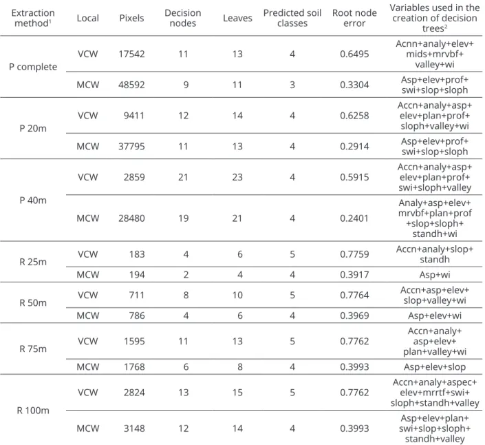
The complexity of a decision tree is a function of the ease for interpretation of its rules, thus its size and the number of variables used in modeling will reveal their level of complexity. Table 2 compares the number of training pixels, the decision nodes, root node error, predicted soil classes, number of leaves and the variables used in the creation of the decision trees for each watershed.
The most complex decision trees (the ones with greater number of leaves + decision nodes, and that consequently enabled a larger number of rules for soil class prediction) were those generated from PM methods, including the complete polygon and the elimination of 20 and 40 m from their boundaries, for both watersheds, in accordance with the greater number of training pixels. They were also the ones that had the best overall accuracy in comparison with those generated from BP methods (discussed later). The latter, in general, were smaller and with fewer rules, presenting lower overall accuracy. This is in accordance with Caten, Dalmolin and Ruiz (2012) who also found better predictive power through more complex decision trees.
The best decision trees generated for VBW could not formulate rules for the RL class, which means that the set of information extracted from the RL pedological mapping unit was not enough for training the trees or that its terrain information was very similar in relation to the terrain information of other soil classes. For MCW, only the decision tree generated from the information of the complete polygons (total area) omitted the
identification of the CX class. The other decision trees
were able to predict all soil classes present in this watershed.
In this study, the number of training pixels
may have been reflective on the predictive power of
the generated trees, as those generated from the PM methods, containing greater number of training pixels,
(1) 1 = =
∑
c j xjj OA Nwherein: xjj is the number of correct samples and N is the
total number of samples.
KI is an agreement measure that uses all elements of a confusion matrix. Their values may range from smaller than 0 (suggesting disagreement) to a maximum of 1 (excellent agreement). According to Landis and Koch (1977), KI is classified as: no agreement (<0), slight (0 - 0.19), fair (0.20 to 0.39), moderate (0.40 to 0:59), substantial (0.60 - 0.79) and excellent (0.80 - 1.00) agreement and is calculated by the Equation 2:
(2) 1 1 2 1 = = = − = −
∑
∑
∑
c c j j c jN xjj xjixij
KI
N xjixij
in which: KI is the estimate of the Kappa index; xij is the value in a row i and in a column j; xji is sum of values in line i; xij is the sum of values in column j; N is the total
number of samples (points used for validation); and c is the number of soil classes. From the calculations of OA
and KI, it was possible to define the method of extraction
of information and, hence, the soil map predicted with the greatest accuracy for each watershed.
Extrapolating information to similar surrounding areas and validation
Table 2: Number of training pixels, decision nodes, root node error, number of predicted soil classes, leaves and
variables used in the creation of the decision trees using the different extraction methods for the Vista Bela creek (VBW) and Marcela Creek (MCW) watersheds.
Extraction
method1 Local Pixels
Decision
nodes Leaves
Predicted soil classes
Root node error
Variables used in the creation of decision
trees2
P complete
VCW 17542 11 13 4 0.6495
Acnn+analy+elev+ mids+mrvbf+
valley+wi
MCW 48592 9 11 3 0.3304 Asp+elev+prof+swi+slop+sloph
P 20m
VCW 9411 12 14 4 0.6258
Accn+analy+asp+ elev+plan+prof+
sloph+valley+wi
MCW 37795 11 13 4 0.2914 Asp+elev+prof+
swi+slop+sloph
P 40m
VCW 2859 21 23 4 0.5915
Accn+analy+asp+ elev+plan+prof+ swi+sloph+valley
MCW 28480 19 21 4 0.2401
Analy+asp+elev+ mrvbf+plan+prof +slop+sloph+
standh+wi
R 25m VCW 183 4 6 5 0.7759
Accn+analy+slop+ standh
MCW 194 2 4 4 0.3917 Asp+wi
R 50m VCW 711 8 10 5 0.7764 Accn+asp+elev+slop+valley+wi
MCW 786 4 6 4 0.3969 Asp+elev+wi
R 75m VCW 1595 11 13 5 0.7762
Accn+analy+ asp+elev+ plan+valley+wi
MCW 1768 6 8 4 0.3993 Asp+elev+slop
R 100m
VCW 2824 13 15 5 0.7762
Accn+analy+aspec+ elev+mrrtf+swi+ sloph+standh+valley
MCW 3148 12 14 4 0.3993
Asp+elev+plan+ swi+slop+sloph+ standh+valley
1P = polygon, P 20 and 40 m = 20 and 40 m eliminated from the polygon edges, R = distance (radii) from the sample points; 2ACCN = altitude above the channel network, analy = analytical hill-shading, asp = aspect, elev = elevation, mrrtf = multiresolution index of ridge top flatness, mrvbf = multiresolution index of valley bottom flatness, mids = mid-slope position, plan = plan curvature, prof = profile curvature, swi = SAGA wetness index, slop = slope, sloph = slope height, standh - standardized height, valley = valley depth, wi = wetness index.
had smaller prediction error rates than those generated from BP methods, and these contained smaller amounts of training data. These results are in agreement with
The most often used terrain attributes by decision trees for the distinction of soil classes in VBW were: altitude above the channel network, analytical hill shading, valley depth, elevation, plan curvature and wetness index. Comparing the use of terrain attributes per method, for the PM methods, only slope and mrrtf were not used, while
for BP methods, SAGA wetness index, mrvbf, profile
curvature, midslope position and slope height were not used in any decision tree. In VCW, most Latosols, the dominant soils in the area, tend to occur on undulated topography, whereas CX and RL are more commonly found on strong undulated topography. RY, in turn, are found in areas of lower altitude above the channel network, lower elevation and greater wetness index, typical of places closer to the water courses (Menezes et al., 2009). It is worth to draw attention to the fact that slope gradient was not used by decision trees to model VCW soils, although it is considered one of the most commonly used terrain attributes to be related to soil classes and properties (Brown, McDaniel and Gessler, 2012; Heung et al., 2016; Kheir et al., 2010; Silva et al., 2014) and one of the most easily perceived terrain attributes during soil surveys, which illustrates the importance of other terrain attributes to help explain soils distribution across the landscape.
For MCW, the most used terrain attributes were aspect, elevation, SAGA wetness index, slope height and topographic wetness index. According to the use of terrain attributes per method, for the PM method, 4 terrain attributes were not used (AACN, mrrtf, midslope position and valley depth), while in the BP method, 6 terrain
attributes were not used: AACN, mrvbf, mrrtf, profile
curvature, analytical hillshading and midslope position. The terrain attributes AACN, mrrtf and midslope position were not used in any method. On the other hand, elevation,
profile curvature, slope and slope height were used in all
decision trees for the PM method, whereas for BP method, no terrain attribute was common for all decision trees of this method, except for aspect, that was used by all the decision trees for MCW including both methods. This fact demonstrates that, contrary to VCW, in MCW terrain attributes that are more easily perceived on the landscape
during soil surveys, such as elevation, slope and profile curvature can help to define the places of occurrence of
the soil classes in MCW. It is important to draw attention to the fact that the analysis of only one terrain attribute is
not enough for defining the places where each soil class
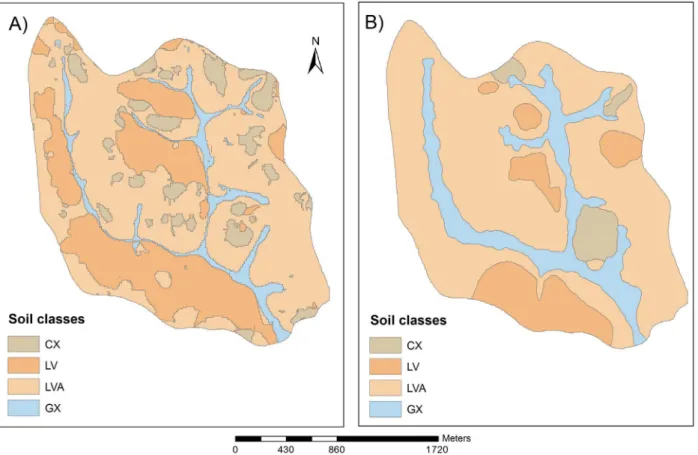
might occur. Thus, the combination of terrain attributes is necessary for a better determination of their places on the landscape. Decision trees that generated maps with greater accuracy (analysis and validation of the maps in further section) are shown in Figure 3.
Soil maps generated from decision trees and their accuracy
Table 3 shows the accuracy of maps generated by all the decision trees created. The soil maps that were generated based on BP methods showed lower accuracy compared to the PM method in VBW and greater in MCW. In the case of VBW, this is probably due to the sampling scheme employed in the study area during the conventional soil mapping that included sites in transitional zones between soil classes for determining the boundaries of the mapping units so that the polygons were delineated. Thus, the points used for the buffers are mostly located in transition regions between soil classes, which may have affected the modeling in the procedure of extracting information. In addition, an adequate contribution of predictor variables for these transitional locations in modeling the decision trees may be diminished because of the less precise delineation of polygons at the creation of the soil map, as stated by Caten, Dalmolin and Ruiz (2012), which may also have contributed to the lower accuracy of this method as a basis for extracting information in VCW. Legros (2005) compared the delineation of mapping units made by different
pedologists, finding out that the polygons present common
areas, but the boundaries tend to be more divergent since they are transitional zones between soil classes.
The maps generated by the elimination of uncertainty areas (polygon boundaries) in VBW had better contribution of the predictor variables and, hence, soil maps with greater accuracy than those obtained from both the PM method extracting information from the complete polygon and the BP methods, which did not consider transition zones between soil classes. Analyzing the two methods that disregarded the polygon boundaries, method P 20 had better accuracy and was the best in predicting soil classes for VBW (Table 3 and Figure 4A).
For MCW, most maps generated by the BP methods had greater accuracy than the same method used for the VBW. In MCW, the sampled points presented in the conventional map, used in this work for creation of buffers for extraction of soil information and creation of decision trees, are mostly located at representative
places of soil classes, where soil profiles were analyzed
Figure 3: Decision trees generated from exclusion of 20 m from the polygon boudaries (A) and (B) buffer of 25
m from the sampled points, respectively for Vista Bela creek (VCW) and Marcela creek (MCW) watersheds. Elev = elevation; Asp = aspect; AACN = altitude above the channel network; Wi = wetness index; Valley = valley depth; Analy = analytical hill shading; Plan = plan curvature; Prof = profile curvature; Sloph = slope height.
the soil map and are allowed to contain inclusions of other soil classes that differ from the dominant in the polygons (IGBE, 2015), which may have hindered the modeling of soil classes by decision trees and consequent less accuracy
Table 3: Overall accuracy (OA) and kappa index (KI) of the predicted soil maps generated from decision trees created by different methods of extracting information from conventional soil maps.
Watersheds
Vista Bela creek Marcela creek
Method1 KI1 OA2 Method KI OA
P complete 0.1971 45% P complete -0.0417 50%
P 20m 0.3525 55% P 20m 0.0955 55%
P 40m 0.2517 45% P 40m 0.0805 60%
R 25m 0.0635 30% R 25m 0.2424 50%
R 50m 0.1195 30% R 50m 0.1882 45%
R 75m -0.0260 20% R 75m 0.1235 45%
R 100m 0.0790 30% R 100m 0.0769 40%
1 P = polygon, P 20 and 40 m = 20 and 40 m eliminated from the polygon edges, R = distance (radii) from the sample points.
Although the predicted maps did not present very high accuracies, they were consistent with other studies that used decision trees as a support for soil mapping (Caten, Dalmolin and Ruiz 2012; Giasson et al., 2006; Giasson et al., 2011).
Extrapolation of soils information to
environmentally similar areas surrounding the watersheds and their validation
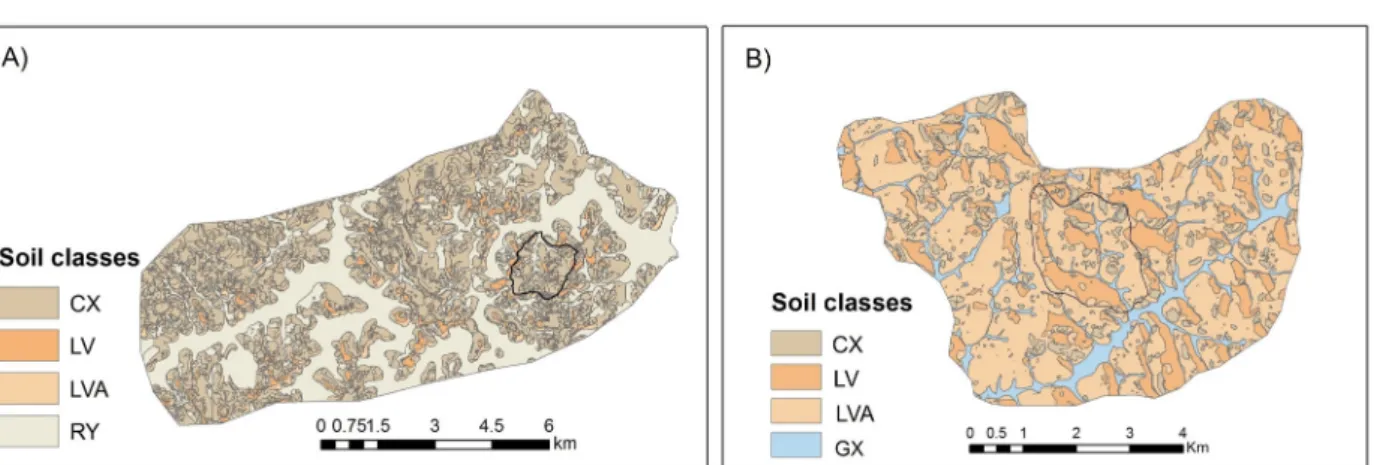
The best decision trees obtained for the watersheds were used as a basis for extrapolating information for their surrounding areas with similar environmental conditions. The map generated for the surroundings of the VCW (Figure 6a) presented validation indices of 40% for OA and KI of 0.1176, which were lower than those resulted from the application of the decision tree rules to the very
same area of VCW (Table 3). However, these findings are
expected because the extrapolated area is 36 times larger than the area of the VCW (reference area).
For the soil map of the MCW surrounding area (Figure 6b), OA and KI were, respectively, 58.33% and 0.2683, being both greater than those obtained for the area of the watershed (Table 3), indicating an improvement on the generated map for this watershed, although the extrapolated area is 9.5 times greater than the MCW area.
These results support the potential of decision trees for the extraction of information from existing maps and extrapolation to larger areas with environmental conditions similar to those of the reference areas. Comparing the area of the watersheds with the area of extrapolation, much information was obtained, with
less time spent and lower financial costs compared to
conventional mapping. Therefore, these digital soil mapping techniques have demonstrated to be both useful and in accordance with the Brazilian reality of scarcity of
financial resources to create more detailed soil surveys
for large areas.
Figure 5: A) Map generated by the decision tree obtaining information from buffers of 25 m radius from the
CONCLUSIONS
The methods of extracting information from soil maps by removing uncertainty areas contributed to better modeling and prediction of the occurrence of soil classes across the landscape by using decision trees. The use of soil legacy data with support of digital mapping techniques is a quicker manner to obtain information and it is a suitable alternative to understand the pedologist’s mental model extracted from analog conventional maps. Obtaining information through decision trees allows for the extrapolation of soil maps for regions surrounding the reference areas containing similar environmental conditions.
ACNOWLEDGEMENTS
The authors would like to thank CNPq, CAPES and
FAPEMIG for providing the financial support necessary
for carrying out this work.
REFERENCES
BENDIX, J. Geländeklimatologie. Berlin: Gebrüder Borntraeger, 2004. 282p.
BEVEN, K.; KIRKBY, N. A physically based variable contributing area model of basin hydrology. Hydrological sciences Bulletin. 24:43-69, 1979.
BÖHNER, J.; MCCLOY, K. R.; STROBL, J. SAGA - Analysis and Modeling Applications. Göttinger Geographische Abhandlungen. 115:1-130, 2006.
BREIMAN, L. et al. Classification and regression trees (CART). Belmont: Wadsworth International, 1984. 358p.
BROWN, R. A.; MCDANIEL, P.; GESSLER, P. E. Terrain attribute modeling of volcanic ash distributions in Northern Idaho. Soil Science Society of America Journal. 76:179-187, 2012. BUI, E. N. Soil survey as a knowledge system.
Geoderma.120:17-26, 2004.
BUI, E. N.; MORAN, C. J. Disaggregation of polygons of surficial geology and soil maps using spatial modelling and legacy data. Geoderma, 103:79-94, 2001.
CATEN, A. T.; DALMOLIN, R. S. D.; RUIZ, L. F. C. Digital soil mapping: strategy for data pre-processing. Revista Brasileira de Ciência do Solo. 36:1083-1091, 2012.
CURI, N.; CHAGAS, C. S.; GIAROLA, N. F. B. Distinção de ambientes agrícolas e relação solo-pastagens nos Campos da Mantiqueira, MG. In: CARVALHO, M. M.; EVANGELISTA, A. R.; CURI, N. (Eds.). Developments of Pastures in Physiographical Region of Campos das Vertentes, MG. Coronel Pacheco: EMBRAPA, 1994, p.21-44.
DIETRICH, H.; BÖHNER, J. Cold air production and flow in a low mountain range landscape in hessia (Germany). Hamburger Beiträge zur Physischen Geographie und Landschaftsökologie. 19:37-55, 2008.
FAVROT, J. C. A strategy for large scale soil mapping: the reference areas method. Science du Sol. 27:351-368, 1989.
GALLANT, J. C.; DOWLING, T. I. A multiresolution index of valley bottom flatness for mapping depositional areas. Water Resources Research. 39:1347-1359, 2003.
GALLANT, J. C.; WILSON, J. P. Primary topographic attributes. In: WILSON, J. P.; GALLANT, J. C. (Eds.). Terrain Analysis: Principles and applications. New York: John Wiley & Sons, 2000, p.51-85.
GIAROLA, N. F. B. et al. Solos da região sob influência do
reservatório da hidrelétrica de Itutinga/Camargos
(MG): perspectiva ambiental. Lavras: CEMIG/UFLA/FAEPE, 1997. 101p .
GIASSON, E. et al. Digital soil mapping using multiple logistic regression on terrain parameters in southern Brazil. Scientia Agricola. 63:262-268, 2006.
GIASSON, E. et al. Decision trees for digital soil mapping on subtropical basaltic steeplands. Scientia Agricola. 68:167-174, 2011.
GIASSON, E. et al. Instance selection in digital soil mapping: A study case in Rio Grande do Sul, Brazil. Ciência Rural, 45:1592-1598, 2015.
GREVE, M. H. et al. Comparing decision tree modeling and indicator kriging for mapping the extent of organic soils in denmark. Digital Soil Mapping: Bridging research, environmental application, and operation. Progress in Soil Science, 2010, v.2, p.267-280.
HEUNG, B. et al. An overview and comparison of machine-learning techniques for classification purposes in digital soil mapping. Geoderma. 266:62-77, 2016.
IBGE. Manual técnico de pedologia. Rio de Janeiro: IBGE, 2015. 430p.
KHEIR, R. B. et al. Predictive mapping of soil organic carbon in wet cultivated lands using classification-tree based models: The case study of Denmark. Journal of Environmental Management. 91:1150-1160, 2010.
LANDIS, J. R.; KOCH, G. G. The measurement of observer agreement for categorical data. Biometrics. 33:159-174, 1977.
LEGROS, J. P. Mapping of the soil. Enfield: Science Publisher, 2005. 411p.
LOH, W. Y. Classification and regression trees. Data Mining Knowledge Discovery. 1:14-23, 2011.
MAIMON, O.; ROKACH, L. Data mining and knowledge discovery handbook. 2ed. New York: Springer New York Dordrecht Heidelberg London, 2010, 1306 p.
MENDONÇA-SANTOS, M. L.; SANTOS, H. The state of the art of Brazilian soil mapping and prospects for digital soil mapping. In: LAGACHERIE, P.; McBRATNEY, A. B.; VOLTZ, M. (Eds). Developments in Soil Science. New York: Elsevier, 2007, v.31, p.39-54.
MENEZES, M. D. et al. Levantamento pedológico e sistema de informações geográficas na avaliação do uso das terras
em sub-bacia hidrográfica de Minas Gerais. Ciência e Agrotecnologia. 33:1544-1553, 2009.
MOTTA, P. E. F. et al. Levantamento pedológico detalhado, erosão dos solos, uso atual e aptidão agrícola das
terras de microbacia piloto na região sob influência
do reservatório da hidrelétrica de Itutinga/Camargos-MG. Lavras: UFLA/CEMIG, 2001. 51p.
R DEVELOPMENT CORE TEAM. R: A language and environment for statistical computing. 2015. Vienna: R Foundation for Statistical Computing. Available in: <http://www.r-project. org>. Access in: April, 26, 2015.
RESENDE, M. et al. Pedologia: base para distinção de ambientes. 6. ed. Lavras: Editora UFLA, 2014, 378p.
ROUDIER, P.; BEAUDETTE, D. E.; HEWITT, A. E. A conditioned Latin hypercube sampling algorithm incorporating operational constraints. In: MINASNY, B. et al. (Eds.). Digital soil assessments and beyond. Netherlands: CRC Press/ Balkema, 2012. p.227-232.
SCHAETZL, R.; ANDERSON, S. S o i l s : g e n e s i s a n d geomorphology. New York: Cambridge University Press, 2015, 817 p.
SCULL, P.; FRANKLIN, J.; CHADWICK, O. A. The application of classification tree analysis to soil type prediction in dessert landscape. Ecological Modelling. 181:1-15, 2005.
SILVA, S. H. G. et al. A technique for low cost soil mapping and validation using expert knowledge on a watershed in Minas Gerais, Brazil. Soil Science Society of America Journal. 78:1310-1319, 2014.
SILVA, S. H. G. et al. Retrieving pedologist’s mental model from existing soil map and comparing data mining tools for refining a larger area map under similar environmental conditions in Southeastern Brazil. Geoderma. 267: 65-77, 2016.
THERNEAU, T.; ATKINSON, B.; RIPLEY, B. Rpart: Recursive Partioning and Regression Trees. 2015. Avalible in:<http:// cran.r-project.org/web/packages/rpart/rpart.pdf>. Access in: January, 21, 2016.
UFV - CETEC - UFLA - FEAM. Mapa de solos do Estado de Minas Gerais. Belo Horizonte: Fundação Estadual do Meio Ambiente, 2010, 49p.