A Framework for Exploratory Analysis of Extreme Weather Events Using
Geostatistical Procedures and 3D Self-Organizing Maps
Jorge Gorricha, Victor Lobo
CINAVEscola Naval Almada, Portugal
lourenco.gorricha@marinha.pt, vlobo@isegi.unl.pt
Ana Cristina Costa
ISEGI-UNLUniversidade Nova de Lisboa Lisboa, Portugal ccosta@isegi.unl.pt
Abstract— Extreme weather events such as heavy precipitation can be analyzed from multiple perspectives such diverse as the daily intensity or the number of consecutive wet days. Thus, it is necessary to get an overall view of the problem in order to characterize the extreme precipitation occurrence along time and space. Extreme precipitation indices, estimated from the empirical distribution of the daily observations, are increasingly being used not only to investigate trends in observed precipitation records, but also to examine scenarios of future climate changes. However, each of the indices, by itself, shows only a part of the phenomenon and there are multiple examples where one single index is not sufficient to characterize the occurrence of extreme precipitation. Therefore, a high dimensional approach should be considered. In this paper, we propose a framework for characterizing the spatial patterns of extreme precipitation that is based on two types of visualization approaches. The first one uses linear models, such as Ordinary Kriging and Ordinary Cokriging, to produce continuous surfaces of five extreme precipitation indices. The second one uses a three-dimensional Self-Organizing Map to visualize the phenomenon from a global perspective, allowing identification and characterization of spatial patterns and homogeneous areas. Also, to allow an easy interpretation of spatial patterns, a pattern matrix is proposed, where variables and color patterns are ordered using a one-dimensional Self-Organizing Map. The proposed framework was applied to a set of precipitation indices, which were computed using daily precipitation data from 1998 to 2000 measured at nineteen meteorological stations located in Madeira Island. Results show that the island has distinct climatic areas in relation to extreme precipitation events. The northern part of the island and the higher locations are characterized by heavy precipitation events, whereas the south and northwest parts of the island exhibit low values in all indices. The promising results from this study indicate that the proposed framework, which combines linear and nonlinear approaches, is a valuable tool to deepen the knowledge on local spatial patterns of extreme precipitation.
Keywords-Climate; Kriging; Precipitation patterns; Self-Organizing Map; 3D Self-Self-Organizing Map.
I. INTRODUCTION
The occurrence of extreme weather events, such as extreme precipitation, is usually associated to an increase of risk for some human activities. Therefore, the monitoring of risk associated with such phenomena is a key element in
ensuring safety, economic development and sustainability of human activities.
Some extreme weather events, such as heavy precipitation, can be analyzed from multiple perspectives as diverse as the daily intensity of precipitation or the number of consecutive wet days. Moreover, those perspectives often have overlapping effects. Thus, when characterizing the occurrence of extreme precipitation, it is necessary to get a synoptic perspective of the phenomenon, considering all its dimensions. This work extends our earlier work on extreme precipitation in Madeira Island [1] regarding the use of Geostatistical Procedures and a Three-Dimensional (3D) Self-Organizing Map (SOM) [2-5] to visualize multidimensional spatial data.
To get a uniform view on observed changes in precipitation extremes, a core set of standardized indices was defined by the joint working group CCI/CLIVAR/JCOMM Expert Team on Climate Change Detection and Indices (ETCCDI) [6]. Some of these indices correspond to the enunciated perspectives of extreme precipitation. This kind of climate data has, at least, two major problems: first, as stated before, each of the indices, by itself, shows only a part of the problem; second, precipitation indices are typically measured in meteorological stations and, therefore, it is necessary to estimate the values of those indices in areas that are not covered by meteorological stations.
Extreme precipitation events can be characterized and analyzed using multiple approaches. Numerous studies of changes in extreme weather events focus on linear trends in the indices, aiming to determine whether there has been a statistically significant shift in such indices [7-10], but only a few focus on their local spatial patterns [11].
In this paper, we propose a framework for the exploratory analysis of extreme precipitation events that is based on two types of approaches: the first one uses linear models, such as Ordinary Kriging and Ordinary Cokriging, to produce continuous surfaces of five extreme precipitation indices; the second one uses a 3D SOM to visualize the phenomenon from a global perspective, i.e., in all its dimensions, allowing the identification and characterization of homogeneous areas and the detection of spatial patterns.
To illustrate the effectiveness of the proposed framework, we present a case study of precipitation events in Madeira Island, which is a Portuguese subtropical island located in the North Atlantic. It is considered a
Mediterranean biodiversity 'hot-spot' and is especially vulnerable to climate change [12]. During the winter season, eastward moving Atlantic low-pressure systems bring precipitation to the island and stationary depressions can cause extreme precipitation events [12]. The characterization of precipitation in Portuguese islands has been less studied than in mainland Portugal [8].
The work reported herein investigates the spatial patterns of extreme precipitation in Madeira Island during three hydrological years (1998-2000). Amongst the eleven precipitation indices proposed by the ETCCDI, five indices were selected, hoping to achieve a global characterization of the phenomenon in its different perspectives. The selected indices capture not only the precipitation intensity, but also the frequency and length of heavy precipitation events. Although the period chosen is not significant for a robust characterization of extreme precipitation events in Madeira Island, it is sufficient to test the proposed framework and provide an exploratory analysis of the phenomenon.
First, for spatial interpolation purposes, the spatial continuity models of the five precipitation indices were computed using geostatistical procedures, such as Ordinary Kriging (OK) and Ordinary Cokriging (OCK). Finally, the estimated surfaces of all the precipitation indices were analyzed using a clustering tool especially adapted for visualizing multidimensional data: the SOM.
This paper is organized into five sections as indicated: Section II presents the related work; Section III presents the framework; Section IV provides an example covering the proposed framework; Section V reports some concluding remarks.
II. RELATED WORK
Looking for spatial patterns and homogeneous zones is an important field of study in climatology. The aim of this paper is demonstrate that 3D SOM can be a valuable tool when it is used together with some well known geostatistical procedures, such as Kriging, in order to detect homogeneous zones and spatial patterns associated to some extreme weather events, such as heavy precipitation.
The use of SOM has brought a new approach to climate analysis that allows us to circumvent some limitations of traditional approaches [13], such as Principal Component Analysis (PCA). A typical example of this was demonstrated by comparing SOM and PCA in the extraction of spatial patterns in Reusch et al. [14]. In fact, that work demonstrates that PCA can fail to extract spatial patterns in cases where SOM performs well.
Identifying homogeneous zones and spatial patterns is one of the major fields of application of SOM in climate analysis and we can find multiple examples of such applications in the literature. For instance, in Hsu and Li [15], SOM is used to recognize homogeneous hydrologic regions and for the identification of the associated precipitation characteristics. Guèye et al. [16] propose the use of SOM, combined with a hierarchical ascendant classification to compute, using the mean sea level pressure and 850 hPa wind field as variables, the main synoptic weather regimes relevant for understanding the daily
variability of rainfall. In more recent work, SOM is applied to, objectively, identify spatially homogeneous clusters [15]. In Gorricha and Lobo [17], the use of SOM is proposed for the visualization of homogeneous zones using border lines computed according to the distances in the input data space. In Lin et al. [18], the SOM is applied to identify the homogeneous regions for regional frequency analysis, showing that the SOM can identify them more accurately when compared to other clustering methods.
However, the use of SOM in climate analysis is not restricted to spatial patterns recognition. The literature is also rich in other examples, such as the use of the SOM to classify atmospheric patterns related with extreme rainfall [19], the use of SOM to identify synoptic systems causing extreme rainfall [20] and some other examples of using the SOM in climate studies, such as analysis of circulation variability, evolution of the seasonal climate and climate downscaling [13, 21].
Because the SOM converts the nonlinear statistical relationships that exist in data into geometric relationships, able to be represented visually [3, 4], it can be considered as a visualization method for multidimensional data, especially adapted to display the clustering structure [22, 23], or in other words, as a diagram of clusters [3]. When compared with other clustering tools, the SOM is characterized mainly by the fact that, during the learning process, the algorithm tries to guarantee the topological ordering of its units, thus allowing an analysis of proximity between the clusters and the visualization of their structure [24].
Typically, a clustering tool must ensure the representation of the existing patterns in data, the definition of proximity between these patterns, the characterization of clusters and the final evaluation of the output [25]. In the case of spatial data, the clustering tool should also ensure that the groups are made in line with geographical closeness [24]. The geo-spatial perspective is, in fact, a crucial point that makes the difference between spatial clustering and clustering in common data. Recognizing this, there are several approaches, including some variants to the SOM algorithm [26], proposed to visualize the SOM in order to deal with geo-spatial features. In this context, an alternative way to visualize the SOM taking advantage of the very nature of geo-referenced data can be reached by coloring the geographic map with label colors obtained from SOM units [24]. One such approach is the “Prototypically Exploratory Geovisualization Environment” [27] developed in MATLAB®. This prototype incorporates the possibility of linking SOM to the geographic representation by color, allowing dealing with data in a geo-spatial perspective.
In this study, we propose to use a clustering method for spatial data based on the visualization of the output space of a 3D SOM [28]. The proposed approach is based on the association of each of the three orthogonal axes (x, y and z) that define the SOM grid output space to one of the three primary colors: red, green and blue (RGB scheme). The results obtained in Gorricha and Lobo [28] point to a significant increase in the clustering quality due to use of 3D SOMs, when compared with the most usual SOMs, i.e., defined with a regular two-dimensional (2D) grid of nodes.
III. DATA ANALYSIS FRAMEWORK
The framework used in this study integrates two main steps: first, the values of each index (variable) at unsampled locations are estimated using geostatistical procedures; second, the indices (variables) are visualized using the SOM. A. Geostatistical modeling of precipitation indices
As the ultimate goal is to get an insight of the spatial patterns of extreme precipitation, the first step is the spatial interpolation of each primary variable (index averaged over the study period). Geostatistical methods, known as Kriging, are usually preferred to estimate unknown values at unsampled locations because they account for the attribute’s spatial continuity.
In this study, we will focus on two particular cases of this group of linear estimators: the OK and the OCK. The main difference between these two Kriging variants is that OCK explicitly accounts for the spatial cross-correlation between the primary variable and secondary variables [29].
A key step of Kriging interpolation is the spatial continuity modeling, which corresponds to fitting an authorized semivariogram model (e.g., Exponential, Spherical, Gaussian, etc.) to the experimental semivariogram cloud of points [29]. This procedure is extremely important for structural analysis and is essential to get the Kriging parameters [30]. The modeling results of this stage will be detailed in the next Section.
The methodology used to model the spatial continuity of each index can be summarized as follows:
Determine the experimental semivariogram for the two main directions of the island’s relief orientation (if there is significant evidence of geometric anisotropy). Isotropy can be assumed only if the semivariogram is not dependent on direction [31]; In the remaining cases assume isotropy;
If there is evidence of strong correlation and linear relationship between some primary variable and the existing secondary information (i.e., elevation), the model of co-regionalized variables is considered in the semivariogram modeling phase.
After modeling the experimental semivariograms, the OK/OCK methods are applied. The interpolation model selected to describe each index will be chosen based on the Mean Error (ME) of the cross-validation (or "leave-one-out" cross-validation) results. This criterion is especially appropriate for determining the degree of bias in the estimates [32], but it tends to be lower than the real error [33]. Therefore, the final decision will also consider the Root Mean Square Error (RMSE) of the cross-validation results, which is an error statistic commonly used to check the accuracy of the interpolation method.
B. Using the SOM to Visualize the Precipitation Indices After producing the spatial surface of each averaged precipitation index, the main goal is to visualize this set of variables in order to identify areas with similar patterns of occurrence of extreme precipitation. To achieve this, we
propose the use of the SOM, a data visualization tool that has been proposed for visualizing spatial data [34, 35].
The SOM is an artificial neural network based on an unsupervised learning process that performs a gradual and nonlinear mapping of high dimensional input data onto an ordered and structured array of nodes, generally of lower dimension [4]. In its most usual form, the SOM algorithm performs a number of successive iterations until the reference vectors associated to the nodes of a bi-dimensional network represent, as far as possible, the input patterns that are closer to those nodes (vector quantization). In the end, every input pattern in the data set is mapped to one of the network nodes (vector projection). As a result of this process, by combining the properties of an algorithm for vector quantization and vector projection, the SOM compresses information and reduces dimensionality [36].
After this optimization process, topological relations amongst input patterns are, whenever possible, preserved through the mapping process, allowing the similarities and dissimilarities in the data to be represented in the output space [3]. Therefore, the SOM algorithm establishes a nonlinear mapping between the input data space and the map grid that is called the output space.
Formally, let us consider a 3D SOM defined with three dimensions [u v w] and a rectangular topology. The SOM grid or the output space (N) is a set of (u × v × w) units (nodes) defined in R3, such that:
N{ni [xy z]T R3:i1,2,...,(uvw)} (1) where x, y and z are the unit coordinates in the output space, such that: ) 1 ( ,..., 1 , 0 ) 1 ( ,..., 1 , 0 ) 1 ( ,..., 1 , 0 w z v y u x (2)
These coordinates must be adjusted to fit the RGB values, which typically vary between 0 and 1. The new coordinates (R,G,B) of the unit ni in RGB space can be obtained through
the range normalization of the initial values:
1 ; 1 ; 1 w z B v y G u x R (3)
As a result, each of the three dimensions of the 3D SOM will be expressed by a change in tone of one particular primary color (RGB) and, hence, each SOM unit will have a distinct color label. This process allows that each geo-referenced element can receive the color of its Best Matching Unit (BMU), i.e., the SOM unit where each geo-referenced element is mapped. Fig. 1 represents schematically a SOM with 27 units (3×3×3) in the RGB space followed by the geographical representation of several geo-referenced elements painted with the color labels of their BMU’s.
Figure 1. Linking SOM’s knowledge to cartographic representation. A color is assigned to each SOM unit (following the topological order). Then the geo-referenced elements are colored with the color of their BMU’s.
The visualization strategy proposed in Fig. 1 is also adaptable to explore the SOM output space of SOMs defined with only two dimensions, indeed the most usual form. However, this visualization strategy, based on the association of an RGB color to each output space dimension of the SOM, clearly won with the use of 3D SOMs.
C. Framework Diagram
In this subsection, we present a diagram (Fig. 3) that summarizes the proposed framework for exploratory analysis of extreme weather events that are characterized by several variables measured in some meteorological stations along time (several years).
The framework will encompass three major phases: - Data extraction and preprocessing;
- Estimation of values at unsampled locations using OK and OCK, including the Geo-statistical modeling of variables along space;
- Visualization of the high dimensional spatial data using the SOM.
IV. THE CASE OF MADEIRA ISLAND
A. Study Region And Data
This subsection provides a description of the study region and of the data used to characterize extreme precipitation patterns in Madeira Island in order to illustrate the framework proposed in Section II.
1) Madeira Island
The study area corresponds to Madeira Island, which is located in the Atlantic Ocean between latitudes 32° 30' N – 33° 30' N and longitudes 16° 30' W – 17° 30' W. The island has an area of approximately 737 km2 distributed over a mountain range of 58 km oriented in the direction WNW-ESE (Fig. 2).
The climate of the island is extremely influenced by the Atlantic Azores anticyclone and also by its own characteristics of altitude and relief direction [37]. In fact, the island’s topography orientation causes a barrier, almost perpendicular to the most frequent wind direction (northeast). As a result of this natural barrier, there is a continuous ascent of moist air masses from the Atlantic, causing frequent precipitation in the northern part of the island [37].
Figure 2. Madeira’s island elevation model.
Despite the small size of the island, there are significant differences in the climate of its two halves [38]: the northern part of the island is colder and wetter; the southern part is warmer and drier. Also, as expected, the precipitation on the island increases with altitude but presents significant differences between those two halves.
FRAMEWORK DIAGRAM
1. DATA PREPROCESSING PHASEThe final data matrix is obtained with the mean values of each variable measured at the p meteorological stations.
In this phase it is necessary to identify the variables that allow characterizing the phenomenon and the meteorological stations where those variables are measured along time.
2. ESTIMATION OF VALUES AT UNSAMPLED LOCATIONS
For each variable it is necessary to choose the best model for spatial interpolation. The spatial continuity models will be found through the experimental semivariograms.
One model per variable will be chosen using cross validation methods generating a raster model.
3. VISUALIZATION OF SPATIAL DATA
Variable 1 Variable 2 (…) Variable n The raster model of each variable will be used in a
3D SOM
Each geo-referenced element (raster cell) receives the color of its Best Matching Unit (3D SOM Output space)
To allow an easy interpretation a pattern matrix is proposed where variables and color patterns are ordered using a 1D SOM. Also, by applying a color scheme to the values of each variable we can easily identify the colors that represent high (red), mean (yellow) and low (green) values of each variable.
The highest annual precipitation occurs in the highest parts of the island and the lower rainfall amounts are observed in lowland areas, such as Funchal and Ponta do Sol [39].
2) Precipitation indices
The daily precipitation data used to compute the indices were observed at 19 meteorological stations of the National Information System of Hydric Resources (NISHR) in the period 1998–2000 (Fig. 4) and downloaded from the NISHR database (http://snirh.pt). In the present study, only annually specified indices are considered. A wet day is defined as a day with an accumulated precipitation of at least 1.0 mm. The precipitation indices computed on an annual basis can be described as follows:
R1 is the number of wet days (in days);
Rx1d is the maximum 1-day precipitation (in mm); CWD is the maximum number of consecutive wet
days (in days);
SDII is named simple daily intensity index and is equal to the ratio between the total rain on wet days and the number of wet days (in mm/day);
Rx5d is the highest consecutive 5–day precipitation total (in mm).
Some of the selected indices are part of a variable set that is widely used in rainfall-extremes analysis and for recognition of the associated spatio-temporal patterns [40].
The precipitation data used in the subsequent analysis corresponds to the simple annual average of each index from October 1998 to September 2000, at each station location. Summary statistics of these data are presented in Table I. The combined analysis of the 5 indices allows characterizing extreme precipitation situations under different perspectives, namely considering the intensity, length and frequency of the precipitation events.
The data and ancillary information used in this study, particularly the island map and its Terrain Digital Elevation Model (Fig. 2) were downloaded from the Instituto Hidrográfico website and from the GeoCommunity™ portal, respectively.
Figure 4. Distribution of meteorological stations over the island (NISHR network).
TABLE I. SUMMARY STATISTICS OF THE PRECIPITATION INDICES
VALUES AVERAGED IN THE PERIOD 1998–2000
Variable (days) CWD (days) R1 (mm) Rx1d (mm/day) SDII Rx5d (mm)
Min 5 52 50 8 64 Median 9 104 114 15.00 216 Max 15 141 169 26 390 Mean 9.53 94.95 114.74 15.48 218.2 Standard-deviation 3.1 27.47 35.0 4.26 92.9 Skewness 0.44 -0.25 -0.06 1.11 0.18 Kurtosis -0.77 -1.22 -1.22 2.15 -0.63 B. Results
In this subsection, we present the spatial interpolation of the precipitation indices and the spatial patterns of extreme precipitation obtained using the methodology proposed in the previous Section.
Deterministic interpolation methods, such as Inverse Distance Weighting (IDW), were not considered because these methods produce inaccurate results when applied to clustered data [32]. Actually, not only the number of stations is small, but also the stations are not distributed equally over the island.
One possible way to try to reduce the problem is through the use of secondary information. In this study, we used the elevation model of Madeira Island as secondary information since some primary variables are strongly correlated with elevation.
1) Spatial interpolation of precipitation indices
The semivariogram modeling was conducted using the GeoMS® software and the spatial prediction models were obtained using ARCGIS®. The final visualization of the extreme precipitation was produced through routines and functions implemented in MATLAB®.
Not surprisingly, the most correlated indices are Rx1d and Rx5d. The remaining indices are moderately or weakly correlated, which indicates their suitability to characterize different features of the precipitation regime in Madeira Island. Moreover, Rx5d and CWD are moderately correlated with elevation (Table II).
TABLE II. CORRELATION MATRIX BETWEEN INDICES AND
ELEVATION (ELEV.)
Variables Elev. CWD R1 Rx1d SDII Rx5d
Elev. 1 CWD 0.768 1 R1 0.424 0.684 1 Rx1d 0.393 0.242 0.489 1 SDII 0.308 -0.134 -0.098 0.627 1 Rx5d 0.616 0.440 0.542 0.804 0.62 1
Taking into account the results obtained in the exploratory analysis (IDW models not shown), several
modeling strategies were compared considering the spatial continuity behavior assumed for each index and its correlation with elevation (Table III). Although the relief of the island has a WNW-ESE direction, the analysis of the estimated surfaces obtained with IDW shows no evidence of anisotropy, except for variable Rx5d. This means that the spatial variability of all other indices was assumed identical in all directions (i.e., isotropic).
TABLE III. EXPERIMENTAL SEMIVARIOGRAM MODELING STRATEGIES
Index model number Semivariogram Spatial behavior assumed CWD-1 Omnidirectional Isotropic
CWD-2 Linear model of
co-regionalization with elevation Isotropic
R1 Omnidirectional Isotropic
Rx1d Omnidirectional Isotropic
SDII Omnidirectional Isotropic
Rx5d-1 Omnidirectional Isotropic
Rx5d-2 Semivariogram models for the
azimuth directions 100º and 10º Anisotropic
Rx5d-3 Linear model of co-regionalization with elevation Isotropic
Table IV summarizes the semivariogram parameters estimated for the models indicated in Table III through the experimental semivariograms. An example of fitting a model to an experimental semivariogram to choose the model of spatial continuity is shown in Fig. 5.
TABLE IV. SEMIVARIOGRAM PARAMETERS ESTIMATED FOR THE
MODELS INDICATED IN TABLE III
Index model number
Model type Nugget Partial sill Spatial
range (Km) CWD-1 Spherical 6 3 11.7 CWD-2 Exponential (Exp.) 0 9 (CWD) 940 (CWD-Elevation) 166272 (Elevation) 13.4 R1 Exp. 0 714 12.6 Rx1d Exp. 0 1157 8.2 SDII Exp. 0 17 5.3 Rx5d-1 Gaussian 1165 6992 12.7 Rx5d-2 Gaussian 1371 6794 14.3 (major) 8.2 (minor) Rx5d-3 Spherical 0 6440 (Rx5d) 23891 (Rx5d-Elevation) 166380 (Elevation) 12.6
OCK with elevation was used in the spatial interpolation of the averaged Rx5d and CWD, whereas all other variables were interpolated through OK (Figs. 6-9).
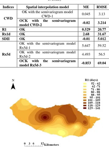
The final interpolation model selected to describe the spatial distribution of Rx5d and CWD depends on the error statistics of the cross-validation presented in Table V. In this case, we opted for a "leave-one-out" cross-validation strategy, where sample values are deleted from the dataset, one at the time. Then, the interpolation method is applied to
estimate the missing value using the remaining observed values. Once the process is complete, the estimation errors were calculated as the differences between estimated and observed values. ME values close to zero indicate a small bias in the estimation. Hence, the best interpolation strategy for both variables is OCK with the semivariogram models Rx5d-3 and CWD-2, respectively.
Figure 5. Example of a Semivariogram: variable R1 assuming isotropic behaviour.
TABLE V. CROSS-VALIDATION ERROR STATISTICS OBTAINED IN THE
VARIOUS SPATIAL INTERPOLATION STRATEGIES (SELECTED MODELS ARE IN BOLD)
Indices Spatial interpolation model ME RMSE
CWD
OK with the semivariogram model
CWD-1 0.045 3.13
OCK with the semivariogram
model CWD-2 -0.02 3.214
R1 OK 0.529 20.77
Rx1d OK 2.68 31.67
SDII OK -0.01 5.012
Rx5d
OK with the semivariogram model
Rx5d-1 5.647 59.52
OK with the semivariogram model
Rx5d-2 4.493 56.5
OCK with the semivariogram
model Rx5d-3 -0.853 69.04
(a) (b) Figure 7. OK interpolation: (a) Averaged Rx1d index; (b) Averaged SDII index.
(a) (b) (c)
Figure 8. Interpolation of the averaged Rx5d index using: (a) OK and the semivariogram model Rx5d-1; (b) OK and the semivariogram model Rx5d-2; (c) OCK and the semivariogram model Rx5d-3.
(a) (b)
Figure 9. Interpolation of the averaged CWD index using: (a) OK and the semivariogram model CWD-1; (b) OCK and the semivariogram model CWD-2.
2) Spatial patterns of extreme precipitation
In order to visualize the spatial patterns of extreme precipitation from a global perspective, a 3D SOM was applied to the indices surfaces obtained through Kriging. First, the selected models (Table V), obtained in raster format, were converted back to point data, sampled at regular intervals. Afterwards, the indices values were normalized to
ensure equal variance in all variables and the SOM was parameterized as follows:
The output space was set with 3 dimensions [4 × 4 × 4], which corresponds to 64 units in total;
The neighborhood function selected was Gaussian; The length of the training was set to “long” (8
epochs);
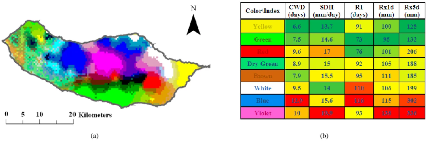
(a) (b)
Figure 10. Visualization of the five precipitation indices: (a) Cartographic representation of data using the output of the SOM mapped to a 3D RGB space. Areas with similar colors have similar characteristics. (b) Matrix of Patterns. This representation of the values in table VII allows to interpret the colors of spatial patterns and is obtained by the ordination of variables and patterns (colors) according to the euclidean distance between those variables and patterns
and by using a color schemma to express high/low values of the variable (green-yellow-red).
As the final results depend on the initialization of the SOM, 100 models were obtained and the best model was chosen according to the criterion of best fit, i.e., the lowest quantization error (Table VI).
TABLE VI. 3DSOMRESULTS (100MODELS)
Quantization Error Topological Error
Selected Model 0.117 0.010
Average Model 0.123 0.045
A RGB color was assigned to each unit of the SOM (output space of the network) according to its output space coordinates. In turn, each raster cell was represented cartographically with the color assigned to the unit of the SOM where that cell is mapped, i.e., its BMU (Fig. 10 (a)). This means that each color corresponds to a homogeneous zone in terms of the various indices values.
Table VII summarizes the characteristics of each area identified in Fig. 10. There are significant differences between the different areas (colors). Table VII allows comparing the predicted mean values for the whole island.
Although the colors in Fig. 10 (a) have a precise meaning, it is recognized that reading Fig. 10 (a) simultaneously with the values of Table VII is not easy. In fact, it will be much more difficult if many variables (and colors) are available for analysis. With this in mind, we also propose the matrix pattern in Fig. 10 (b), based on Table VII, to facilitate the interpretation of the map in Fig. 10 (a).
This matrix is the result of a one-dimensional ordering of the variables and color patterns that characterize each of the areas shown in Fig.10 (a). Within the array of patterns each cell receives one color depending on the value of the variable: low values of the variable are represented by a
green color, average values are represented by a yellow color and high values are represented by a red color.
TABLE VII. SUMMARY OF THE AVERAGE VALUES FOR EACH AREA
Color\Index CWD (days) R1 (days) Rx1d (mm) SDII (mm/day) Rx5d (mm) Yellow 6.6 91 100 13.7 125 Violet 10 93 138 19.9 336 Red 9.6 76 101 17 206 Blue 12.9 116 115 15.6 302 White 9.5 110 106 14 199 Dry Green 8.9 92 105 15 188 Green 7.5 73 95 14.6 132 Brown 7.9 95 111 15.5 185
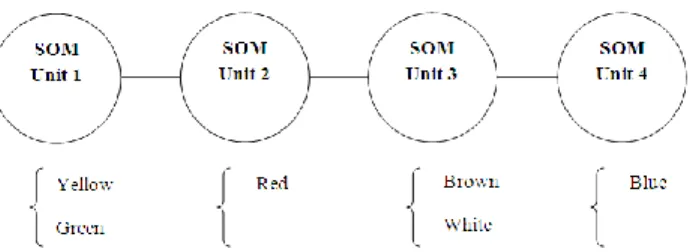
Thus, by applying a color scheme to the values of each variable we can easily identify the colors that represent high (red), mean (yellow) and low (green) values of each variable. To perform the ordering of the variables and color patterns we also used SOM. However, in this case, the SOM was defined only with a single output space dimension. In fact, because of its own features, SOM is not only a clustering method; it performs an ordering that depends on its output space dimension. If the SOM is defined with one single dimension, colors will be represented by one single SOM unit in the output space as represented in Fig. 11. Thus colors will be ordered. The same strategy applies to variables; each variable will be mapped to one single SOM unit that has a specific order in the output space.
The colors and variables of the matrix pattern in Fig. 10 (b) are ordered according to the results in Table VIII.
Figure 11. This figure represents schematically an example of a SOM with an output space definied with one single dimension with four units. All
colors (or variables) will be mapped to one single unit so they will be ordered in the output space of the SOM.
TABLE VIII. ORDINATION PROCESS OF VARIABLES AN COLOR
PATTERNS REPRESENTED IN FIG.10
Color SOM unit
(best match unit) Variables
SOM Unit (best match unit) Yellow 1 CWD 1 Violet 3 R1 5 Red 6 Rx1d 10 Blue 8 SDII 15 White 10 Rx5d 20 Dry Green 13
SOM definied with one single dimension (1X20)
Green 16
Brown 20
SOM definied with one single dimension (1X20)
Thus, interpreting the matrix pattern in Fig. 10 (b), we can say that despite its small size, Madeira Island has distinct zones in relation to extreme precipitation events. The violet area and blue area correspond to the higher regions of the island characterized by higher values in all indices, whereas the yellow area (in the far east of the island) is characterized by the lowest values in all indices. The north of the island, which is colored blue and white, corresponds to high values in all indices (although much smaller than in the violet colored area), with particularly high R1 index values. Finally, the area colored in green is characterized by low values in all indices and broadly corresponds to Funchal city. The dry green area is very close to the average values (a phenomenon that is partly explained by the lack of information in the area). There are no significant differences between the green and brown zones.
Another important aspect that can be extracted from Fig. 10 (a) is the transition zone between green and violet/blue area. In fact, if we had used a traditional clustering method we would probably get the distinct areas but not the transition zones.
V. CONCLUSION
In this paper, we propose a framework for characterizing the spatial patterns of extreme weather events exemplified by the exploratory analysis of extreme precipitation events in Madeira Island. This framework combines two different approaches: the first one is based on geostatistical procedures and the second one is based on the 3D SOM. The first
approach is used to estimate spatial surfaces of extreme precipitation indices. The second one allows visualizing the phenomenon from a global perspective, thus, enabling the identification of homogeneous areas in relation to extreme precipitation events.
The proposed framework is specially adapted to an exploratory analysis of high dimensional spatial data via visualization. The results show that it is possible to identify the relevant spatial patterns that exist in data, thus allowing gaining new knowledge about data. Another important issue is that the proposed framework does not impose a priori hypothesis about the number of clusters. In fact, the clustering structure emerges naturally without any previous definition. Moreover, not only the clusters emerge visually but also the transition zones between homogeneous zones became evident. This is, in fact, a crucial point and is actually a huge advantage since it is going to match exactly the reality of the area: spatial changes occur but gradually, not abruptly.
The spatial and temporal resolution of the data set considered in this example is too small to thoroughly characterize the extreme precipitation phenomenon in Madeira Island. Nevertheless, the results indicate the proposed framework as a valuable tool to provide a set of maps that can effectively assist the spatial analysis of a phenomenon. It can have multiple perspectives and deal with high dimensional data requiring a global view. The results of this particular application open perspectives for new applications not only in the climate context, but also in other domains where it is necessary to analyze high dimensional spatial patterns.
REFERENCES
[1] J. Gorricha, V. J. A. S. Lobo, and A. C. Costa, "Spatial Characterization of Extreme Precipitation in Madeira Island Using Geostatistical Procedures and a 3D SOM," in
Proceedings of the 4th International Conference on Advanced Geographic Information Systems, Applications, and Services - GEOProcessing 2012, Valencia, Spain, 2012, pp. 98-104.
[2] T. Kohonen, "The self-organizing map," Proceedings of the
IEEE, vol. 78, pp. 1464 -1480, 1990.
[3] T. Kohonen, "The self-organizing map," Neurocomputing, vol. 21 pp. 1-6, 1998.
[4] T. Kohonen, Self-organizing Maps, 3rd ed. New York: Springer, 2001.
[5] T. Kohonen, "Essentials of the self-organizing map," Neural
Networks, vol. 37, pp. 52-65, 2013.
[6] A. M. G. K. Tank, F. W. Zwiers, and X. Zhang, "Guidelines on Analysis of extremes in a changing climate in support of informed decisions for adaptation," WMO2009.
[7] A. C. Costa and A. Soares, "Trends in extreme precipitation indices derived from a daily rainfall database for the South of Portugal," International Journal of Climatology, vol. 29, pp. 1956-1975, 2009.
[8] M. I. P. de Lima, S. C. P. Carvalho, and J. L. M. P. de Lima, "Investigating annual and monthly trends in precipitation structure: an overview across Portugal," Nat. Hazards Earth
Syst. Sci., vol. 10, pp. 2429-2440, 2010.
[9] G. M. Griffiths, M. J. Salinger, and I. Leleu, "Trends in extreme daily rainfall across the South Pacific and relationship to the South Pacific Convergence Zone,"
International Journal of Climatology, vol. 23, pp. 847-869,
2003.
[10] M. Haylock and N. Nicholls, "Trends in extreme rainfall indices for an updated high quality data set for Australia, 1910–1998," International Journal of Climatology, vol. 20, pp. 1533-1541, 2000.
[11] A. C. Costa, R. Durão, M. J. Pereira, and A. Soares, "Using stochastic space-time models to map extreme precipitation in southern Portugal," Nat. Hazards Earth Syst. Sci., vol. 8, pp. 763-773, 2008.
[12] M. J. Cruz, R. Aguiar, A. Correia, T. Tavares, J. S. Pereira, and F. D. Santos, "Impacts of climate change on the terrestrial ecosystems of Madeira," International Journal of Design and
Nature and Ecodynamics, vol. 4, pp. 413-422, 2009.
[13] B. C. Hewitson, "Climate Analysis, Modelling, and Regional Downscaling Using Organizing Maps," in
Self-Organising Maps: applications in geographic information science, A. Skupin and P. Agarwal, Eds. Chichester, England:
John Wiley & Sons, 2008, pp. 137-153.
[14] D. B. Reusch, R. B. Alley, and B. C. Hewitson, "Relative performance of Self-Organizing Maps and Principal Component Analysis in pattern extraction from synthetic climatological data," Polar Geography, vol. 29, pp. 188-212, 2005.
[15] K.-C. Hsu and S.-T. Li, "Clustering spatial-temporal precipitation data using wavelet transform and self-organizing map neural network," Advances in Water Resources, vol. 33, pp. 190-200, 2010.
[16] A. K. Guèye, S. Janicot, A. Niang, S. Sawadogo, B. Sultan, A. Diongue-Niang, and S. Thiria, "Weather regimes over Senegal during the summer monsoon season using self-organizing maps and hierarchical ascendant classification. Part II: interannual time scale," Climate Dynamics, vol. 39, pp. 2251-2272, 2012.
[17] J. Gorricha and V. Lobo, "Improvements on the visualization of clusters in geo-referenced data using Self-Organizing Maps," Computers & Geosciences, vol. 43, pp. 177-186, 2012.
[18] G.-F. Lin and L.-H. Chen, "Identification of homogeneous regions for regional frequency analysis using the self-organizing map," Journal of Hydrology, vol. 324, pp. 1-9, 2006.
[19] T. Cavazos, "Large-Scale Circulation Anomalies Conducive to Extreme Precipitation Events and Derivation of Daily Rainfall in Northeastern Mexico and Southeastern Texas,"
Journal of Climate, vol. 12, p. 1506, 1999.
[20] G. Schädler and R. Sasse, "Analysis of the connection between precipitation and synoptic scale processes in the
Eastern Mediterranean using self-organizing maps,"
Meteorologische Zeitschrift, vol. 15, pp. 273-278, 2006.
[21] B. C. Hewitson and R. G. Crane, "Self-organizing maps: applications to synoptic climatology," Climate Research, vol. 22, pp. 13-26, August 08, 2002 2002.
[22] J. Himberg, "A SOM based cluster visualization and its application for false coloring," in Proceedings of the
IEEE-INNS-ENNS International Joint Conference on Neural Networks, Como, Italy, 2000, pp. 587- 592.
[23] S. Kaski, J. Venna, and T. Kohonen, "Coloring that reveals high-dimensional structures in data," in Proceedings of 6th
International Conference on Neural Information Processing,
Perth, WA, 1999, pp. 729-734.
[24] A. Skupin and P. Agarwal, "What is a Self-organizing Map?," in Self-Organising Maps: applications in geographic
information science, P. Agarwal and A. Skupin, Eds.
Chichester, England: John Wiley & Sons, 2008, pp. 1-20.
[25] A. K. Jain, M. N. Murty, and P. J. Flynn, "Data Clustering: A Review," ACM Computing Surveys, vol. 31, pp. 264-323, 1999.
[26] F. Bação, V. Lobo, and M. Painho, "The self-organizing map, the Geo-SOM, and relevant variants for geosciences,"
Computers & Geosciences, vol. 31, pp. 155-163, 2005.
[27] E. L. Koua and M. Kraak, "An Integrated Exploratory Geovisualization Environment Based on Self-Organizing Map," in Self-Organising Maps: applications in geographic
information science, P. Agarwal and A. Skupin, Eds.
Chichester, England: John Wiley & Sons, 2008, pp. 45-86. [28] J. Gorricha and V. Lobo, "On the Use of Three-Dimensional
Self-Organizing Maps for Visualizing Clusters in
Georeferenced Data " in Information Fusion and Geographic
Information Systems. vol. 5, V. V. Popovich, C. Claramunt, T.
Devogele, M. Schrenk, and K. Korolenko, Eds.: Springer Berlin Heidelberg, 2011, pp. 61-75.
[29] P. Goovaerts, Geostatistics for natural resources evaluation. New York: Oxford University Press, 1997.
[30] P. A. Burrough and R. A. McDonnell, Principles of
Geographical Information Systems. Oxford: Oxford University Press, 1998.
[31] A. D. Hartkamp, K. D. Beurs, A. Stein, and J. W. White, "Interpolation Techniques for Climate Variables," CIMMYT, Mexico1999.
[32] E. H. Isaaks and R. M. Srivastava, An introduction to applied
geostatistics. New York: Oxford University Press, 1989.
[33] I. A. Nalder and R. W. Wein, "Spatial interpolation of climatic Normals: test of a new method in the Canadian boreal forest," Agricultural and Forest Meteorology, vol. 92, pp. 211-225, 1998.
[34] E. L. Koua, "Using self-organizing maps for information visualization and knowledge discovery in complex geospatial datasets," in Proceedings of 21st International Cartographic
Renaissance (ICC), Durban, 2003, pp. 1694-1702.
[35] F. Bação, V. Lobo, and M. Painho, "Applications of Different Self-Organizing Map Variants to Geographical Information Science Problems," in Self-Organising Maps: applications in
geographic information science, A. Skupin and P. Agarwal,
Eds. Chichester, England: John Wiley & Sons, 2008, pp. 22-44.
[36] J. Vesanto, J. Himberg, E. Alhoniemi, and J. Parhankangas,
SOM Toolbox for Matlab 5. Espoo, Finland: Helsinki
University of Techology, 2000.
[37] S. Prada, M. Menezes de Sequeira, C. Figueira, and M. O. da Silva, "Fog precipitation and rainfall interception in the natural forests of Madeira Island (Portugal)," Agricultural and
Forest Meteorology, vol. 149, pp. 1179-1187, 2009.
[38] J. J. M. Loureiro, "Monografia hidrológica da ilha da Madeira," Revista Recursos Hídricos, vol. 5, pp. 53-71, 1984. [39] S. Prada, "Geologia e Recursos Hídricos Subterrâneos da Ilha
da Madeira." vol. PhD: Universidade da Madeira, 2000. [40] H. J. Fowler and C. G. Kilsby, "A regional frequency analysis
of United Kingdom extreme rainfall from 1961 to 2000,"
International Journal of Climatology, vol. 23, pp. 1313-1334,