Automatic Completion of Text-based Tasks

(1)

Daniel Filipe Rodrigues Henriques

Bachelor of Science

Automatic Completion of Text-based Tasks

Dissertation submitted in partial fulfillment of the requirements for the degree of

Master of Science in

Computer Science and Engineering

Advisers: João Freitas, CTO, DefinedCrowd João Moura Pires, Assistant Professor, Faculdade de Ciências e Tecnologia da Universidade Nova de Lisboa

Co-advisers: Rui Correia, Machine Learning Engineer, DefinedCrowd

Filipe Marques, Associate Professor, Faculdade de Ciências e Tecnologia da Universidade Nova de Lisboa

Examination Committee Chairperson: Carlos Damásio

(2)

(3)

Automatic Completion of Text-based Tasks

The Faculty of Sciences and Technology and the NOVA University of Lisbon have the right, perpetual and without geographical boundaries, to file and publish this dissertation through printed copies reproduced on paper or on digital form, or by any other means known or that may be invented, and to disseminate through scientific repositories and admit its copying and distribution for non-commercial, educational or research purposes, as long as credit is given to the author and editor.

This document was created using the (pdf)LA_{TEX processor, based in the “novathesis” template[1], developed at the Dep. Informática of FCT-NOVA [2].}

(4)

(5)

to my beloved parents who gave me everything they had without ever holding back.

(6)

(7)

Ac k n o w l e d g e m e n t s

I would first like to thank my thesis advisers João Freitas and Rui Correia from Defined-Crowd and professors João Moura Pires and Filipe Marques. The development of this thesis took place at DefinedCrowd. As a consequence, both João and Rui had to put a great deal of effort to coordinate their work with my thesis’s orientation. I have learned plenty from the world of ML and NLP due to these two amazing mentors. I would like to give a special thanks to Rui, whose patience is infinite. Thank you for all the reviews, the tips, the corrections, and the healthy discussions. If today I can write a scientific paper is because of you.

However, both my professors have helped me whenever they could. Professor Filipe Marques was vital during the mathematical component of this thesis as his suggestions steer the investigation to a whole different level. Professor João Moura Pires helped me a lot with the visualizations and thanks to its recommendations, the plots in this thesis are not only informative but also beautiful.

I would like to thank the Computer Science Department and FCT for being my second house during this past 5 years. It was an honor to be able to conclude my studies at the best Portuguese engineering university.

I would also like to thank my coworkers at DefinedCrowd, especially, Jorge Ribeiro and Francisco Ganhão. Both of them helped me in this journey, and their support was core to keep pushing forward and conclude this achievement. I would like to give a special thanks to Jorge, who helped me to grow as a data scientist, an (almost) engineer, and a person.

I would also like to thank the friends that have made during this master’s degree. Thanks to André Neves, Filipe Amador, Ivo Rocha, Pedro Almeida, Didier Dias, and Dinis Cabanas. Thank you all for your companionship and your ability to make me laugh.

Last but not least, I would like to profoundly thank my loving family. Thanks, mom and dad for all the sacrifices and for all the love. This degree is my most notorious and best achievement, and I could not have done it without you. I love you now and forever.

(8)

(9)

A b s t r a c t

Crowdsourcing is a widespread problem-solving model which consists in assigning tasks to an existing pool of workers in order to solve a problem, being a scalable alternative to hiring a group of experts for labeling high volumes of data. It can provide results that are similar in quality, with the advantage of achieving such standards in a faster and more efficient manner. Modern approaches to crowdsourcing use Machine Learning models to do the labeling of the data and request the crowd to validate the results.

Such approaches can only be applied if the data in which the model was trained (source data), and the data that needs labeling (target data) share some relation. Further-more, since the model is not adapted to the target data, its predictions may produce a substantial amount of errors. Consequently, the validation of these predictions can be very time-consuming. In this thesis, we propose an approach that leverages in-domain data, which is a labeled portion of the target data, to adapt the model. The remainder of the data is labeled based on these model’s predictions. The crowd is tasked with the generation of the in-domain data and the validation of the model’s predictions. Under this approach, train the model with only in-domain data and with both in-domain data and data from an outer domain.

We apply these learning settings with the intent of optimizing a crowdsourcing pipeline for the area of Natural Language Processing, more concretely for the task of Named En-tity Recognition (NER). This optimization relates to the effort required by the crowd to performed the NER task. The results of the experiments show that the usage of in-domain data achieves effort savings ranging from 6% to 53%. Furthermore, we such savings in nine distinct datasets, which demonstrates the robustness and application depth of this approach.

In conclusion, the in-domain data approach is capable of optimizing a crowdsourcing pipeline of NER. Furthermore, it has a broader range of use cases when compared to reusing a model to generate predictions in the target data.

Keywords: Crowdsourcing, Transfer Learning, Machine Learning, Named Entity Recog-nition, Natural Language Processing

(10)

(11)

R e s u m o

Ocrowdsourcing é um modelo de resolução de problemas que consiste na atribuição de

tarefas a um grupo de trabalhadores para resolver um problema, sendo uma alternativa escalável à contratação de especialistas para classificar grandes volumes de dados. Este modelo é capaz de gerar resultados com qualidade semelhante e de uma forma mais rápida e eficiente. Abordagens recentes aocrowdsourcing utilizam modelos de

Aprendiza-gem Automática para fazer a classificação dos dados que é depois validada pelacrowd.

Tais abordagens só podem ser utilizadas se os dados de treino do modelo (dados fonte) e os dados não classificados (dados objetivo) partilharem alguma relação. Além disso, como o modelo não está adaptado aos dados objetivo, as suas previsões podem conter um elevado número de erros. Por consequência, a validação destas previsões é bastante demorada. Nesta tese, propomos uma abordagem que utiliza dados de domínio, que é uma parte dos dados objetivo que está classificada, para adaptar o modelo que classificará o resto dos dados objectivo. Acrowd tem de gerar os dados de domínio e fazer a validação

das previsões. Nesta abordagem, o modelo é treinado com dados de domínio e com dados de domínio em conjunto com dados de um domínio externo.

Esta abordagem é aplicada com o intuito de otimizar umapipeline de crowdsourcing

para Processamento de Linguagem Natural, mais concretamente, para o Reconhecimento de Entidades Mencionadas (REM). Esta otimização está relacionada com o esforço da

crowd na realização da tarefa de REM. Os resultados das nossas experiências mostram

que o uso de dados de domínio obtém diminuições de esforço que variam de 6% a 53%. Adicionalmente, estas diminuições em nove conjuntos de dados, o que demonstra a ro-bustez e leque de aplicações desta abordagem.

Em suma, a abordagem proposta é capaz de otimizar umapipeline de crowdsourcing

de REM. Além disso, esta abordagem tem um espectro de casos de usos mais abrangente quando comparado às abordagens previamente definidas.

Palavras-chave: Crowdsourcing, Transferência de Conhecimento, Aprendizagem Auto-mática, Reconhecimento de Entidades Mencionadas, Processamento de Linguagem Natu-ral

(12)

(13)

C o n t e n t s

List of Figures xv

List of Tables xxiii

Listings xxxi Glossary xxxiii Acronyms xxxv 1 Introduction 1 1.1 Motivation . . . 1 1.2 Problem Statement . . . 2 1.3 Research Questions . . . 3 1.4 Document Structure. . . 4

2 Background & Related Work 5 2.1 Crowdsourcing. . . 6

2.1.1 Distributed Human Intelligence Tasking . . . 7

2.2 Named Entity Recognition . . . 8

2.2.1 Annotation Schemes . . . 10

2.2.2 Evaluation Metrics . . . 11

2.2.3 Annotated Corpora . . . 12

2.2.4 Machine Learning for NER. . . 14

2.3 Transfer Learning . . . 17

2.3.1 Formal Definition and Taxonomy . . . 17

2.3.2 Applications and Practical Use . . . 19

2.4 Discussion . . . 23

3 Model Adaptation 25 3.1 Implementation of State of the Art NER Model . . . 26

3.1.1 Neural Network Architecture . . . 27

3.1.2 Sanity Check and Word Embeddings Dimension Comparison . . . 28

(14)

C O N T E N T S

3.2.1 Data. . . 29

3.2.2 Baseline . . . 30

3.2.3 In-domain Data Approach . . . 31

3.2.4 ODD for Performance Boosting . . . 34

4 Assessment of Crowd Effort Savings 39 4.1 Statistical Analysis of Time on Task . . . 40

4.1.1 Data. . . 40

4.1.2 Calculation of the Token Processing Speed. . . 42

4.1.3 Definition of the Reading and Annotation Time . . . 47

4.2 Estimation of Crowd Effort Gains . . . 50

4.2.1 Data. . . 50

4.2.2 Baseline . . . 52

4.2.3 Measurement of Gains . . . 52

4.2.4 Index of Saved Actions . . . 57

4.2.5 Simulated Crowdsourcing Scenario . . . 61

5 Conclusions and Future Work 67 5.1 Contributions . . . 69

5.2 Future Work . . . 69

Bibliography 71

A Report on Framework Architecture 77

B Model Adaptation 79

C Assessment of Crowd Effort Savings 89

(15)

L i s t o f F i g u r e s

2.1 A crowdsourcing pipeline consisting of two parts: a generation and a valida-tion step. In the generavalida-tion step, contributors are tasked with the labeling of data and, in the validation step, users proceed to validate and correct, if

necessary, the results of the generation step. . . 8

2.2 UI for the task of NER at Neevo. . . 9

2.3 The IOB annotation scheme. The prefix I denotes entities composed of only one token and the tokens in the middle of entities which are composed of more than two tokens; the prefix O denotes tokens which are not entities; the prefix

B denotes the first token of entities which have more than one token.. . . 10

2.4 The IOE annotation scheme. The prefix I denotes entities composed of only one token and the tokens in the middle of entities which are composed of more than two tokens; the prefix O denotes tokens which are not entities; the prefix

E denotes the last token of entities which have more than one token. . . 10

2.5 The IOBES annotation scheme. The prefix I denotes tokens in the middle of entities which have more than two tokens; the prefix O denotes tokens which are not entities; the prefix B denotes the first token of entities which have more than one token; the prefix E denotes the last token of entities which have more

than one token; the prefix S denotes entities composed of only one token. . . 11

2.6 High level architecture of DL-based systems for NER . . . 14

2.7 Two unsupervised learning algorithms that generate word embeddings: the

CBOW and Skip-gram model. . . 15

2.8 The base model, depicted in a three-layered architecture, of a DL system that

uses Transfer Learning strategies for performance boosting. . . 21

2.9 Transfer models for situations where the task differ in terms of application,

domain, and language. . . 22

3.1 The data splits for Dataset A and Dataset B. Dataset A has a development set to enable the fine tune of the hyper-parameters which are then reused for the

remainder of the experiment. . . 30

3.2 The split of the train data in the IDD approach. The train set, in green, is the actual data used for training and the unseen data, in gray, is the portion of the

(16)

L i s t o f F i g u r e s

3.3 A line plot displaying the MUC score associated with each one of the amounts

of training data for both datasets. . . 34

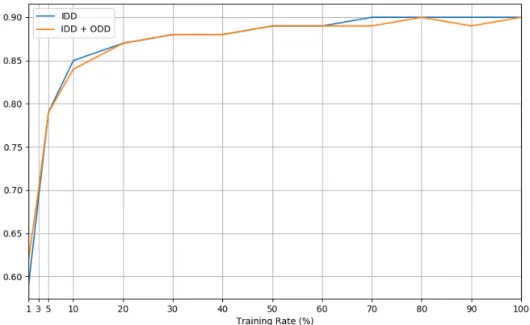
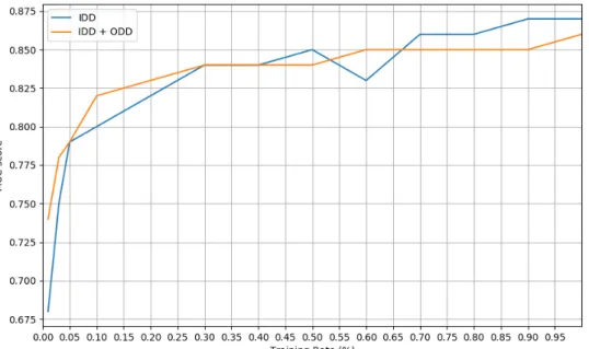
3.4 The values of the MUC score for Model A when trained with in-domain data (blue line) and with in-domain data with the addition of out-domain data (orange line). . . 35

3.5 The values of the MUC score for Model B when trained with in-domain data (blue line) and with in-domain data with the addition of out-domain data (orange line). . . 36

4.1 The bar plots concerning the number of HITs (top) and the number of

contrib-utors (bottom) for each crowdsourcing job. . . 41

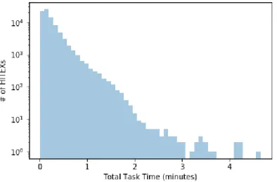
4.2 The distribution of the target variable,totalTaskTime, with the y axis in

loga-rithmic scale. . . 42

4.3 An example of two HITs, one that has no agreement in speed at which it should

be performed (HIT 1) and another that has (HIT 2). . . 44

4.4 The distribution of the target variable,totalTaskTime, after the data cleaning

process. . . 45

4.5 The distribution of the token processing speed after the data cleaning process. 45

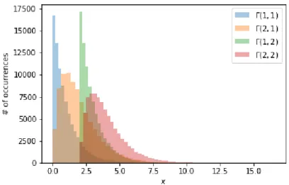
4.6 Four gamma probability density function distributions where the paremeters,

k and θ, vary between 1 and 2. . . . 46

4.7 The distributions of the token processing speed (orange) and the gamma

dis-tribution with the estimated parameters k = 1.5908 and θ = 33.1918 (blue). . 47

4.8 The distributions of the reading speed (orange) and the gamma distribution

with the estimated parameters k = 1.3652 and θ = 71.1587 (blue). . . . 48

4.9 The annotation per entity for each number of annotated entities. This value is

computed by dividing the annotation time by the number of annotated entities. 49

4.10 The same sentence in two distinct scenarios. In scenario A, the sentence is not pre-annotated depicting a generation task. In scenario B, the sentence is pre-annotated depicting a validation task. Note that the pre-annotation in scenario B has an error: the token "Jane" as not been annotated as an entity. . 53

4.11 A line plot with the total effort curves, in minutes, when training the model

with in-domain data (blue line) and in-domain data in conjunction with out-domain data (orange line) when compared against the baseline effort (green

dashed line) for the different amounts of training data. These effort values are

associated with the amounts of training data of CD-1. . . 55

4.12 A line plot with the total effort curves, in minutes, when training the model with in-domain data (blue line) and in-domain data in conjunction with

out-domain data (orange line) when compared against the baseline effort (green

dashed line) for the different amounts of training data. These effort values are

(17)

4.13 The relative effort gains for all crowd datasets for the different amounts of training data.. . . 57

4.14 The curves of the index of saved actions when training the model with only in-domain data (blue line) in-domain data and out-domain data (orange line).

These values are associated with the amounts of training data of CD-1. . . . 58

4.15 The curves of the index of saved actions when training the model with only in-domain data (blue line) in-domain data and out-domain data (orange line).

These values are associated with the amounts of training data of CD-4. . . . 59

4.16 A scatter plot corresponding to the relation between the total effort and the index of saved actions (mapped to the color) when the models are trained using only in-domain data. These values are associated with the amounts of training data of CD-1.. . . 59

4.17 A scatter plot corresponding to the relation between the total effort and the

index of saved actions (mapped to the color) when the models are trained using only in-domain data. These values are associated with the amounts of training data of CD-4.. . . 60

B.1 The values of the MUC score for CD-1 for the different training rates when training the models with in-domain data (blue line) and in-domain data in conjunction with out-domain data (orange line). These values are presented in table B.1.. . . 80

B.2 The values of the MUC score for CD-2 for the different training rates when

training the models with in-domain data (blue line) and in-domain data in conjunction with out-domain data (orange line). These values are presented in table B.2.. . . 81

(18)

C.1 A line plot with the total effort curves, in minutes, when training the model with in-domain data (blue line) and in conjunction with out-domain data

(orange line) when compared against the baseline effort (green dashed line)

for the different amount of training rate. These effort values are associated

with the training rates of CD-1 (see table C.1). . . 90

C.2 A line plot with the total effort curves, in minutes, when training the model

with in-domain data (blue line) and in conjunction with out-domain data (orange line) when compared against the baseline effort (green dashed line)

C.3 A line plot with the total effort curves, in minutes, when training the model with in-domain data (blue line) and in conjunction with out-domain data (orange line) when compared against the baseline effort (green dashed line) for the different amount of training rate. These effort values are associated

C.5 A line plot with the total effort curves, in minutes, when training the model with in-domain data (blue line) and in conjunction with out-domain data

(orange line) when compared against the baseline effort (green dashed line)

(19)

C.10 The curves of the index of saved actions when training the model with only in-domain data (blue line) and in-in-domain data in conjunction with out-in-domain data (orange line). These values are associated with the training rates of CD-1 (see table C.10). . . 99

(20)

C.19 A scatter plot corresponding to the relation between the total effort and the index of saved actions (mapped to the color) when the models are trained using only in-domain data. These values are associated with the training rates of the training rates of CD-1. . . 107

C.20 A scatter plot corresponding to the relation between the total effort and the

index of saved actions (mapped to the color) when the models are trained using only in-domain data. These values are associated with the training rates of the training rates of CD-2. . . 108

C.23 A scatter plot corresponding to the relation between the total effort and the

index of saved actions (mapped to the color) when the models are trained using only in-domain data. These values are associated with the training rates of the training rates of CD-5. . . 109

(21)

(22)

(23)

L i s t o f Ta b l e s

2.1 NER categories and examples. The categories are the ones defined in [24]. . . 9

2.2 Error taxonomy for NER. The "O" indicates the absence of category. . . 11

2.3 A resume of Transfer Learning settings and their relation with the traditional ML approach. The letters "NA" mean indifferent or irrelevant, also the sym-bol 3 for source/target labels means that they are available, thus the symsym-bol

7 should mean the opposite. . . 19

2.4 Depending on the settings and the situation, there is a variety of approaches that can be used. . . 19

2.5 A table showing for each type of transfer the improvement obtained by using

the Transfer Learning approach. . . 21

2.6 Summary of NER datasets. The empty cells are for information that could not

be determined or confirmed. . . 23

3.1 Table with the number of sentences, tokens, and entities for the three data files that compose the CoNLL 2003 English corpus. The category set consisted of

four categories: organization, person, location, and miscellaneous. . . 26

3.2 The probabilities of the wordsice and steam occurring when the words solid,

gas, water, and fashion occur. The ratio of probabilities is also presented to

show words that represent specific properties of the word ice or the word

steam. This table was retrieved from [50]. . . . 27

3.3 Table indicating the obtained F1score for each different dimension of word

embeddings. . . 28

3.4 General metrics regarding the CoNLL 2003 dataset (A) and the financial re-ports corpus (B). . . 29

3.5 The values of precision, recall, F₁ score, MUC score, and support for both

datasets; these values were obtained while training the model with the same

hyper-parameters and dimension of word embeddings and over 50 epochs. . 30

3.6 Values of precision, recall, F1 score, MUC score, and support when using

(24)

L i s t o f T a b l e s

3.7 The number of sentences, tokens, entities, the mean sentence length (number of tokens per number of sentences) and the entity coverage (number of entities per number of tokens) for each amount of training data. These amounts of

training data are associated with the number of sentences of Dataset A. . . . 32

3.8 The number of sentences, tokens, entities, the mean sentence length (number of tokens per number of sentences) and the entity coverage (number of entities per number of tokens) for each amount of training data. These amounts of

training data are associated with the number of sentences of Dataset B. . . . 33

3.9 The relative of gains in performance, measure via MUC score, for each amount of training data of using in-domain data and in-domain data + out-domain

data when compared the pre-trained model approach. . . 35

4.1 The total task time, predicted reading time, and the annotation time per num-ber of annotated entities in a readable format. The reading time was predicted

by recurring to the gamma distribution defined in the previous section. . . . 49

4.2 The number of HITEXs per number of annotated entities. . . 50

4.3 Table with the values of number of HITs, sentences, tokens, categories, and entities associated with each of the crowd datasets. It is also presented two additional computed metrics: average sentence length and entity coverage.

Note that CD stands for crowd dataset. . . 51

4.4 The values of total generation effort for each dataset. These are the efforts

associated when generating the annotations for the entire dataset. . . 52

4.5 The best absolute and relative gains, and the values index of saved actions ρ achieved for each dataset when using the IDD and IDD + ODD approaches. The relative gains range from 6% to 53% and the ρ indicates that the model’s

predictions save more work than what they induced. . . 60

4.6 The absolute and relative gains for 1% of training data, and the values index of saved actions ρ achieved for each dataset when using the IDD and IDD +

ODD approaches. . . 61

4.7 The values of effort for the different amount of training data in terms of the absolute number of HITs for CD-1. These values are associated with training

the models with in-domain data. . . 62

4.8 The values of effort for the different amount of training data in terms of the absolute number of HITs for CD-4. These values are associated with training

4.9 The absolute effort savings, relative effort savings, and index of saved actions for the different amounts of training data. These values are associated with CD-1. . . 62

4.10 The absolute effort savings, relative effort savings, and index of saved actions

for the different amounts of training data. These values are associated with CD-4. . . 63

(25)

4.11 The best absolute and relative gains achieved for each one of the datasets when using only IDD for training the models. The corresponding index of saved actions ρ is also presented. . . . 63

training the models with in-domain data and in-domain data in conjunction

with out-domain data. . . 79

B.2 The values of the MUC score for CD-2 for the different training rates when training the models with in-domain data and in-domain data in conjunction

C.1 The values of generation, validation, and total effort (in minutes) for CD-1 for each distinct training rate value. The validation and total effort are associated to models trained with only in-domain data (blue line) and in-domain data in-domain data in conjunction with out-domain data (orange line). Note that

(26)

the format of the effort is {hours:}:{minutes}. . . 90

C.3 The values of generation, validation, and total effort (in minutes) for CD-3 for

each distinct training rate value. The validation and total effort are associated to models trained with only in-domain data (blue line) and in-domain data in-domain data in conjunction with out-domain data (orange line). Note that

C.6 The values of generation, validation, and total effort (in minutes) for CD-6 for each distinct training rate value. The validation and total effort are associated to models trained with only in-domain data (blue line) and in-domain data in-domain data in conjunction with out-domain data (orange line). Note that the format of the effort is {hours:}:{minutes}. . . 94

(27)

C.10 The values of the index of saved actions when training the model with only in-domain data and in-domain data in conjunction with out-domain data for

the different training rates. These values are associated with CD-1. . . 98

D.1 The values of effort for the different amount of training data in terms of the absolute number of HITs for CD-1. These values are associated with training

D.4 The values of effort for the different amount of training data in terms of the

absolute number of HITs for CD-4. These values are associated with training

(28)

D.10 The absolute effort savings, relative effort savings, and index of saved actions for the different amount of training rates. These values are associated with CD-1. . . 115

D.16 The absolute effort savings, relative effort savings, and index of saved actions

for the different amount of training rates. These values are associated with CD-7. . . 116

D.17 The absolute effort savings, relative effort savings, and index of saved actions

for the different amount of training rates. These values are associated with CD-8. . . 116

(29)

(30)

(31)

L i s t i n g s

3.1 Category mapping function that receives a category from Dataset A and

(32)

(33)

G l o s s a r y

corpus Collection of written texts

(34)

(35)

Ac r o n y m s

AI Artificial Intelligence

BiLSTM bi-directional Long Short Term Memory

CBOW continuous Bag-of-Words CNN Convolutional Neural Network

CoNLL Computational Natural Language Learning CRF Conditional Random Fields

CRL Communication Research Laboratory CV Computer Vision

DL Deep Learning

FN False Negative FP False Positive

GloVe Global Vectors

GRU Gated Recurrent Unit

HIT Human Intelligence Task

HITEX Human Intelligence Task execution HMM Hidden Markov Model

IAA Inter-annotator agreement IDD in-domain data

IOB Inside-Outside-Beginning

IOBES Inside-Outside-Beginning-Ending-Singleton IOE Inside-Outside-Ending

(36)

AC R O N Y M S

LSTM Long Short Term Memory

LSTM-LM Long Short Term Memory-Language Model

MEM Maximum Entropy Model

MET Multilingual Entity Task

ML Machine Learning

MLE maximum likelihood estimation MUC Message Understanding Conference MUC-7 Message Understanding Conference - 7 MUC-6 Message Understanding Conference - 6

NER Named Entity Recognition

NICT National Institute of Information and Communications Technology NLP Natural Language Processing

ODD out-domain data

POS part-of-speech

PTB Penn Treebank

ReLU Rectified Linear Unit RNN Recurrent Neural Network

SGD stochastic gradient descent

SHL-MDNN shared-hidden-layer multilingual Deep Neural Network SVM Support Vector Machine

tpm tokens per minute

UI user interface

WER Word Error Rate

(37)

C

h

a

p

t

e

r

1

I n t r o d u c t i o n

Understanding diversity is imperative to understanding collective intelligence, and collective intelligence is an essential ingredient in one of the primary categories of crowdsourcing: the attempt to harness many people’s knowledge in order to solve problems or predict future outcomes or help direct corporate strategy.

– Jeff Howe

1.1 Motivation

According to Forbes1, 2.5 quintillion bytes of data are generated every day, 95% of which comes in unstructured form [22]. Companies, and organizations in general, have long since recognized the importance of automatically processing this information, to extract meaning from it. In recent years, this information processing has been by resorting to

Machine Learning (ML)algorithms, in particular, supervised learning algorithms. These

algorithms learn from previously labeled input-output pairs, which generates a constant necessity for human labeling in the process of training and refining those models.

Up until the mid-2000s, labeling was mostly done by experts. However, this approach does not scale with the amount of data. Having a large number of experts labeling data is costly; on the other hand, having too few renders the process inefficient. The notion of crowdsourcing emerged as a response to these issues. Howe [31], coined the term as "the act of taking a task traditionally performed by a designated agent (such as an employee or a contractor) and outsourcing it by making an open call to an undefined but large group of people."

1

(38)

C H A P T E R 1 . I N T R O D U C T I O N

Studies show that, for a group of well-defined tasks, the crowd is capable of providing similar quality results when compared to those produced by experts, with the advantage of achieving such standards faster and in a more cost-efficient manner [47,59].

Recent approaches to crowdsourcing introduced a step of pre-labeling which is au-tomatically performed by MLmodels [33,60]. The pre-labeling process is used to im-prove the delivery time and, consequently, the costs associated with the crowd’s effort. These approaches use models to pre-label the data, which is then validated by the crowd. The models are trained on datasets which are already labeled and reused to generate predictions on new non-labeled datasets – henceforth, we refer to this approach as the pre-trained model approach.

However, the pre-trained model approach has constraints when it comes to its ap-plication. The labeled data in which the model is trained needs to be similar or share a relationship with the data to be labeled. Otherwise, the pre-labeling process does not contribute to reducing delivery time, but rather to increase it. Such detail indicates that this process can be optimized.

Companies that rely upon the usage of crowdsourcing to serve its client’s needs have an increased interested in optimizing this process. Often the characteristic of the data and the task that needs to be performed by the crowd depend upon the client’s requirements. Therefore, these companies need to define strategies that allow applyingMLtechniques despite the properties of the data and the underlying task.

1.2 Problem Statement

DefinedCrowd is a startup company that leverages crowdsourcing to fulfill the needs of its clients. DefinedCrowd has a crowdsourcing platform, Neevo, where the crowd can perform data labeling tasks. At DefinedCrowd, the tasks are very heterogeneous as they depend upon the requirements of the clients.

For instance, tasks performed in written text can vary in terms of the label set, the type of text, and the language of the text. Finding a model that is trained on a labeled dataset that corresponds precisely to a client’s requirements is unfeasible and invalidates the possibility of using this approach. A better approach would be to adapt the model to each different task. The following steps indicate how a model can be adapted to a specific task:

1. require the crowd to label only a portion of the data;

2. train a model using only that portion of labeled data;

3. use the model to generate predictions for the remainder of the data;

(39)

1 . 3 . R E S E A R C H Q U E S T I O N S

In this thesis, we investigate the feasibility of this strategy in the area ofNatural

Lan-guage Processing (NLP), more concretely the task ofNamed Entity Recognition (NER).

NERis the task of extracting and annotating words or phrases, in a text, into categories that map to real-world concepts, such as persons, locations, and quantities. At Defined-Crowd, the NER pipeline is one of the most request tasks, which, as a consequence, generates a large amount of data that can be leveraged for our investigation.

In this thesis, we consider a crowdsourcing pipeline that is divided into generation and validation. In the generation step, the crowd is tasked with the annotation of entities in non-annotated unstructured text. In the validation step, the crowd is tasked with the validation of the annotations performed in the generation step.

Therefore, the process of adapting a model to each task has two associated costs: generation and validation. The generation cost relates to the amount of training data, and the validation cost relates to the time the crowd spends correcting the model’s predictions. However, we do not know what which point the model should be trained, and when the generation step should be stopped. Furthermore, we need a way of estimating how much time it takes to generate the training data and how much time it takes to validate the model’s predictions. Having a solution to estimate these costs enables the assessment of the range of optimization that is obtained by leveraging the in-domain approach.

To better understand these issues, one needs to study the relation between the amount of training data and the model’s performance. Herein, we need to understand how does the amount of training data translates into crowd effort during the generation step, and how does the model’s performance translate into crowd effort during the validation.

Ideally, the crowd should generate the least possible amount of training data that allows for training the best possible model to generate predictions for the remainder of the data. Therefore, testing the usage of Transfer Learning falls as a logical path of investigation.

The application of Transfer Learning strategies to the model’s training enables the achievement of better performances while requiring fewer amounts of training data [63,

64]. One such strategy is training the model on two datasets simultaneously, meaning that the model trains with domain data and out of domain data. The domain data is a portion of the data that has been annotated by the crowd, while the out of domain data is a fully annotated dataset.

1.3 Research Questions

The goal of this thesis is the study the relationship between the amount of training, the model’s performance, and the generation and validation costs associated with both these variables. With this in mind, the following research questions were formulated:

• Considering the state of the art regardingNER, how does the amount of training data influence the model’s performance?

(40)

C H A P T E R 1 . I N T R O D U C T I O N

A model trained with a portion of the data can produce better predictions than a pre-trained model. However, it is unclear what is the amount of domain data that should be generated to start the model’s training. The optimum amount of training data is reached when the addition of more data does not contribute significantly to improve the model’s performance.

• How can the in-domain data approach reduce time costs when integrated into a crowdsourcing pipeline?

Answering the first research question provide us with a measure of performance associated with the amount of training data. Herein, we want to estimate the cost of generating that amount of data and estimate the cost of correcting the model’s predictions. Having these costs into consideration enables to determine the point from which the model’s training should be started and measure the extent of the achieve optimizations.

1.4 Document Structure

The remainder of this document is structured as follows:

• Chapter2presents the background and related work for the three main areas in this thesis. First, we present a historical overview and the types of crowdsourcing. We also explain DefinedCrowd’s crowdsourcing platform. The concept ofNERis explained in detail (including formal problem definition, format, and evaluation metrics), and we also the present state of the art solutions regarding this task. The concept of Transfer Learning is also described, as well as its various types and a more thorough description of the application of Transfer Learning toNERis provided;

• Chapter3describes the experiment that answers the first research question. In this chapter, we implement a state of the artNERthat is used to show the relationship between the amount of training data and the model’s performance. We compare these results against the pre-trained model approach;

• Chapter4describes a second experiment, which answers the second research ques-tion. In this experiment, we conduct a statistical analysis to estimate the necessary effort to perform aNERgeneration task. We proceed to assess the efforts associated

with the model’s predictions and present the gains of using our approaches when compared to the traditional crowdsourcing approach;

• Chapter5presents the conclusions and the future work based on the answers of the research questions.

(41)

C

h

a

p

t

e

r

2

Ba c k g r o u n d & R e l a t e d Wo r k

Study the past if you would define the future. – Confucius

Before proceeding with the investigation, we present the related and work and state of the art regarding the concepts of crowdsourcing,NER, and Transfer Learning. Addition-ally, we look into related work that has connected these areas. This chapter is organized as follows:

• Section2.1presents a definition of crowdsourcing, the various types of crowdsourc-ing, the products, and platforms that incorporate this concept and the description of DefinedCrowd’s platform, Neevo1;

• Section2.2presents a definition of theNERtask, how it is performed and evaluated. Following this, we describe a range of datasets related toNER. Then we present automated solutions forNER, starting with ML models that depend upon hand-engineered features and finishing withDeep Learning (DL)-based systems. In the end, state of the art solutions are presented;

• Section2.3 presents a definition and taxonomy of Transfer Learning, as well as applications of this concept to the areas ofComputer Vision (CV), speech, andNLP

that show the advantages of using Transfer Learning.

(42)

C H A P T E R 2 . BAC KG R O U N D & R E L AT E D WO R K

2.1 Crowdsourcing

Crowdsourcing is a widespread problem-solving model which consists of assigning tasks to an existing pool of contributors to solve a problem. Crowdsourcing combines various opinions and answers to reach the problem’s solution. It is possible to trace the informal use of crowdsourcing back to 1714. At that time, the British government created the Lon-gitude Prize, awarding a monetary reward to whoever was able to find the best solution to measure a ship’s longitudinal position at sea [15].

The formal definition of crowdsourcing, however, was first introduced by Howe in 2006 [30]. In his article, Howe presents the iStockphoto2use case and how crowdsourcing changed the stock photography marketplace, by allowing stock photos, whose market value could reach 600 dollars, to be marketed at the one dollar mark. The rationale behind this shift was that professional-grade cameras were starting to cost way less than what they used to and that it was possible to create a crowd of amateurs that could rival professionals. Furthermore, iStockers (contributors of iStockphoto) did not need to profit as much, because this was not their full-time occupation; instead, it was a hobby.

Since 2006, a wide range of companies, universities, and institutions has used crowd-sourcing in a variety of ways, and thus a typology was defined to categorize the different uses of crowdsourcing in today’s applications [8]:

• Knowledge Discovery and Management - the task of finding, collecting, and organiz-ing information into a common location and format. Examples include SeeClickFix3 (a reporting system for citizens to report maintenance needs in their neighborhood) or Wikipedia (a non-profitable organization that centralizes an encyclopedia where the crowd generates and reviews content);

• Broadcast Search - the task of solving empirical problems. Examples include Inno-Centive4(a platform that breaks down problems into challenges that are solved by the crowd to find solutions for these problems);

• Peer-vetted Creative Production - the task of creating and selecting creative ideas. Examples include iStockphoto (a platform that collects stock photos) or LEGO5(the company allowed users to submit new products, via the website, which other users could vote for);

• Distributed Human Intelligence Tasking - the task of analyzing large amounts of information. Examples include Amazon Mechanical Turk6, or Neevo7.

2_{https://www.istockphoto.com/pt (consulted on 11 January 2019).} 3_{https://seeclickfix.com/ (consulted on 18 February 2019).} 4_{https://www.innocentive.com/ (consulted on 18 February 2019).} 5_{https://shop.lego.com/en-GB/ (consulted on 22 February 2019).} 6_{https://www.mturk.com/ (consulted on 22 February 2019).}

(43)

2 . 1 . C R O W D S O U R C I N G

According to the typology above, this thesis is centered around the notion of dis-tributed human intelligence tasking. The remainder of this section details how this crowdsourcing type works.

2.1.1 Distributed Human Intelligence Tasking

The distributed human intelligence tasking is a type of crowdsourcing that aims to pro-cess high volumes of data by resorting to the crowd. This propro-cessing task is, typically, decomposed in tasks, which is the atomic unit of work in this context. These micro-tasks are assigned to a pool of workers that are tasked to complete them. In this section, we describe Neevo, which is a platform that monetarily rewards workers for the comple-tion of these micro-tasks. However, we need to define the terminology and the typical setting of a crowdsourcing pipeline.

The following terminology is based on Neevo. However, it is general enough to de-scribe any crowdsourcing pipeline.

• Contributor - the worker that performs the micro-task;

• Human Intelligence Task (HIT)- the task to be performed by the contributors, each

HITcan be assigned to one or more contributor. Often, we refer to the execution of oneHITby one contributor asHuman Intelligence Task execution (HITEX).

• Job - a collection ofHITs. Each job has an associated type, which indicates the type of tasks to be executed in that job. Types can be related toNLP, such asNERand semantic annotation;CV, such as image collection and image tagging; and speech technologies, such as transcription and speech data collection;

• Project - a collection of jobs. Clients, often ask for complex and specific pipelines that require jobs to be executed one after another. For instance, clients may require the task ofNERto be performed on speech data. However, they do not possess the data. Due to this, the client may require a job of speech data collection followed by a transcription job, and, finally, theNERjob.

Having defined the crowdsourcing taxonomy, we proceed to describe a standard crowdsourcing pipeline. Figure 2.1 shows a standard crowdsourcing pipeline consist-ing of two steps:

• Generation step - the part of the pipeline in which the contributors perform the

HITs. This is the step in which the generation of annotations happens;

• Validation step - the part of the pipeline in which the results of the generation step are validated and, possibly, corrected. It is also possible for this validation step to not be present in a pipeline.

(44)

Figure 2.1: A crowdsourcing pipeline consisting of two parts: a generation and a valida-tion step. In the generavalida-tion step, contributors are tasked with the labeling of data and, in the validation step, users proceed to validate and correct, if necessary, the results of the generation step.

The need for a validation step arises because the crowdsourcing approach allows anyone to solve tasks. Therefore, this validation step is a way of ensuring quality in the results of the generation step [26]. This step is but one approach to ensure that contributors are not malicious or underperforming, and thus ensuring the quality of the results. Two techniques that can be applied to fulfill this goal are: contributor screening and infer contributor’s trust [46].

Contributor screening is the application of a test before starting the job. It can be seen as a qualification test, meaning that a contributor answers a set of questions, and if he gets more than a certain percentage (defined upon job creation), then it is assumed that he is going to perform well. This approach can filter malicious or unskilled contributors even before they start the job, which has the advantage of not having to cancel the results perform by this type of contributors.

Inferring contributor’s trust is the application of tests, that are based on a gold set, during the execution of a task. A gold set is a set of pairs of questions and answers that are known to be right (a ground truth). When the contributors are performing a particular task, they get prompted with these tests that assess the performance of the contributor. Typically, these tests are injected during the execution of theHIT, and contributors do not know that they are being evaluated. If the contributor’s performance starts to decay, he gets excluded from the job, and his results are discarded.

2.2 Named Entity Recognition

The task ofNERwas first introduced by Grishman and Sundheim [24] during theMessage

Understanding Conference - 6 (MUC-6). NERis the task of extracting and classifying

words or phrases, in a text, into categories that map to real-world concepts, such as persons, locations, and quantities. Table2.1depicts the first 7 categories defined for the task ofNERand examples of entities for each categories.

(45)

2 . 2 . N A M E D E N T I T Y R E C O G N I T I O N

Named Entity Example

ORGANIZATION United Nations, The International Maritime Organization PERSON Barack Obama, Marcelo Rebelo de Sousa

LOCATION Portugal, London, Kilimanjaro DATE March 5, 1996; Today; 10/4/2017 TIME 5 AM, midday, 23:40

MONEY 55 euros, $12, 109 ¥ PERCENT 14%, a quarter, a half

Table 2.1: NER categories and examples. The categories are the ones defined in [24].

Figure 2.2: user interface (UI)for the task ofNERat Neevo.

NERis a common task that is often used as an intermediate step for the completion of more complex tasks, such as question answering and summarization.

Figure2.2illustrates an example of aUIfor the task ofNERat Neevo. The users can click and drag to select the part of the text that they wish to tag. After selection, the user can choose a category from the drop-down list. This action can be executed as many times as necessary and, when there is nothing else to annotate, the user can click next and annotate the following text.

NERis an area where a wide range of work has been performed and, for that reason, there was the need to define annotation schemes to perform this task and evaluation metrics to assess the quality of the results. In this section, we define the annotation schemes, the evaluation metrics, and automatic approaches to the problem used in the task ofNER.

(46)

Alex

I-PER

O

is

going

O

to

O

Los

Angeles

B-LOC

I-LOC

Figure 2.3: The IOB annotation scheme. The prefix I denotes entities composed of only one token and the tokens in the middle of entities which are composed of more than two tokens; the prefix O denotes tokens which are not entities; the prefix B denotes the first token of entities which have more than one token.

Alex

I-PER

O

is

going

O

to

O

Los

Angeles

I-LOC

E-LOC

Figure 2.4: The IOE annotation scheme. The prefix I denotes entities composed of only one token and the tokens in the middle of entities which are composed of more than two tokens; the prefix O denotes tokens which are not entities; the prefix E denotes the last token of entities which have more than one token.

2.2.1 Annotation Schemes

From a practical standpoint, the goal ofNERis the classification of each token or phrase in a text. With this in mind, theNERcommunity developed and created consensus around a set of annotation schemes. The annotations generated by these schemes are also tailored to be used as training data toMLalgorithms. In each scheme, a token is classified with a label consisting of a prefix and the category they belong. This prefix is used to relate the token with the structure of the entity. Examples of these schemes are:

• Inside-Outside-Beginning (IOB)(figure2.3) - the prefix I denotes singleton entities,

which are entities composed of only one token, and the tokens in the middle of entities which are composed of more than two tokens; the prefix O denotes tokens which are not entities; the prefix B denotes the first token of entities which have more than one token. A variation calledIOB2 uses the prefix B to denote singleton entities;

• Inside-Outside-Ending (IOE)(figure2.4) - as in theIOBformat, the I and O prefixes

are used in the same context. The prefix E denotes the last token of entities which have more than one token. A variation called IOE2 uses the E prefix to denote singleton entities;

• Inside-Outside-Beginning-Ending-Singleton (IOBES)(figure2.5) - all the prefixes

described previously apply in the same situations in this annotation scheme. When a label is composed of more than two tokens, it starts with the prefix B and ends with the prefix E. Singleton entities are denoted with the prefix S.

(47)

2 . 2 . N A M E D E N T I T Y R E C O G N I T I O N

Alex

S-PER

O

is

going

O

to

O

Los

Angeles

B-LOC

E-LOC

Figure 2.5: The IOBES annotation scheme. The prefix I denotes tokens in the middle of entities which have more than two tokens; the prefix O denotes tokens which are not entities; the prefix B denotes the first token of entities which have more than one token; the prefix E denotes the last token of entities which have more than one token; the prefix S denotes entities composed of only one token.

Error Explanation Output Correct Output

False Negative (FN) The system

misses an entity Robert (O) Robert (I-PER)

Category + Boundary

The system predicts an entity with the wrong label and boundaries in (B-PER) New (I-PER) York (I-PER) New (B-LOC) York (I-LOC) Boundary The system predicts an entity with the wrong boundaries George (B-PER) R. (I-PER) George (B-PER) R. (I-PER) R. (I-PER) Martin (I-PER) Category The system predicts an entity with the wrong label John (B-LOC) Briggs (I-LOC) John (B-PER) Briggs (I-PER) False Positive (FP) The system predicts an entity where it should have not done it

Unlike (I-LOC) Unlike

Table 2.2: Error taxonomy forNER(adapted from [45]). The "O" indicates the absence of category.

2.2.2 Evaluation Metrics

The task ofNERcan be solved automatically by recurring toMLsystems. Therefore, it was necessary to have systematic measures that could represent the quality of these systems and compare performance between them. Before moving to measure performance, it is essential to define which type of errors may arise in what concernsNER.

Table2.2shows a taxonomy ofNER[45]. This taxonomy has five different types of errors. AFNis an entity that should have been predicted by the system, but it was not. The opposite of this error is theFP. The remainder of the errors relates to the category and boundaries of entities. Given this errors, we present three general metrics that measure model performance in classification problems – precision, recall, and F1 score – and the score which has been developed to measure performance inNERtasks, theMessage

(48)

Understanding Conference (MUC)score.

Precision is the percentage of named entities that were classified correctly by the system. Note that, for an entity to be considered correct, it needs to have both category and boundary correct. It can be calculated using equation2.1.

precision = CN E

CN E + W N E (2.1)

In equation2.1, CN E stands for correct named entities, and W N E stands for wrong named entities. Another metric is the recall, which is the percentage of true entities predicted by the system, and it can be calculated using equation2.2.

recall = CN E

CN E + U N E (2.2)

In equation2.2, U N E stands for an unclassified named entity. Having the precision and recall, we can compute the harmonic between the two metrics, which is the F1score, by using equation2.3.

F1= 2 ·

precision · recall

precision + recall (2.3)

However, these metrics do not account for each one of the errors in table2.2because the errors associated with the category and boundaries of the entity assume that entities can be partially correct. For instance, aFNmeans that both category and boundaries are wrong, which implies that predicting either the category or boundaries correctly should contribute to improving the overall score.

This necessity allowed the creation of the MUC score8 which is a micro-averaged F1 score. In this score, named entities are considered correct according to two values: the type (category) and the text (boundaries). Having a two-axis evaluation means that any entity can be considered partially correct if either the type of the text is correct; consequently, this score takes into consideration the errors in table2.2. The final score is calculated as the F₁ score. E.g., for the phrase depicted in figure2.3, not classifying the tokenLos as a location would produce a precision of 0.75 and a recall of 0.75, which

produces aMUCscore of 0.75; computing this by recurring to the traditional definition of precision, recall, and F₁score would produce the values 0.5, 0.5, and 0.5, respectively.

2.2.3 Annotated Corpora

Throughout the years a wide range of datasets has been proposed to solve specific tasks related to them, or to evaluate the performance of NER systems. In this section, we present a brief description ofcorporathat are relevant toNER.

The MUC-6 was the first conference ever to define a NER task. The task defined

consisted of classifying news reports about labor contract negotiations and corporate

8_{An implementation of this score can be consulted on https://github.com/jantrienes/nereval (consulted}