Dynamics of a Gyrostat Satellite with the Vector of Gyrostatic Moment along the Principal Plane of Inertia

UNIVERSIDADE DA BEIRA INTERIOR

Engenharia

Dynamics of a Gyrostat Satellite with the Vector

of Gyrostatic Moment along the Principal Plane

of Inertia

(versão corrigida após defesa)

Pedro Afonso Gomes Dias

Dissertação para obtenção do Grau de Mestre em

Engenharia Aeronáutica

(Ciclo de estudos integrado)

Orientador: Prof. Doutor Luís Filipe Ferreira Marques Santos

Orientador: Prof. Doutor André Resende Rodrigues da Silva

Agradecimentos

Primeiro que tudo, quero agradecer à minha família, em especial aos meus pais e irmãos, que me deram a possibilidade de estudar nesta universidade e por todo o apoio e força, ao longo de todo este tempo.

Em seguido quero dar um agradecimento especial ao meu orientador, Professor Doutor Luís Filipe Ferreira Marques Santos, por me ter sempre ajudado com todos os tipos de problemas que ocorreram ao longo desta investigação, a qualquer hora do dia. Agradeço todas as sugestões, conhecimento, conselhos e disponibilidade que houve da sua parte.

Quero também agradecer ao Professor Doutor André Resende Rodrigues da Silva pela sugestão do tema desta dissertação e, por me ter ajudado em todas as questões colocadas no início deste trabalho.

À Universidade da Beira Interior, ao departamento de Ciências Aeroespaciais e à cidade da Covilhã, agradeço o facto de me terem acolhido e permitido estudar no curso de Engenharia Aeronáutica ao longo destes cinco anos.

Por fim, e não menos importante, quero agradecer a todos os meus amigos, o apoio, o companheirismo e a amizade ao longo de todo o meu percurso académico. Quero ainda deixar um agradecimento especial, a quem me deu dormida quando já não tinha quarto alugado na Covilhã.

Resumo

Satélites artificias são uns dos componentes cruciais da vida moderna. O estudo do controlo da atitude e estabilização de um satélite é necessário para assegurar uma missão bem-sucedida. Existem dois tipos de métodos de estabilização: os métodos passivos e os métodos ativos.

Nesta dissertação é investigado a dinâmica de um satélite tipo giróstato, sujeito a um método semi-passivo de estabilização, nomeadamente o momento gravítico e as propriedades giroscópicas de rotores, ao longo de uma órbita circular.

No caso particular, quando o vetor de momento girostático está ao longo de um dos principais planos de inércia do satélite. Para resolver este problema é proposto um modelo matemático numérico-analítico para determinar todos as posições de equilíbrio de um satélite giróstato, em um sistema coordenado orbital em função das componentes adimensionais do vetor de momento girostático (𝐻𝑖 𝑖 = 1,2,3) e do parâmetro inercial adimensional 𝑣. As condições de existência das soluções de equilíbrio são obtidas. As condições suficientes de estabilidade para cada grupo de soluções de equilíbrio são derivadas, a partir da análise do integral de energia generalizado como uma função de Lyapunov.

O estudo da evolução da bifurcação do equilíbrio foi realizado em detalhe em função do parâmetro 𝑣. Também, a evolução das soluções de equilíbrio em função dos ângulos do satélite é analisada e é verificado a existência de pequenas regiões de 12 e 16 posições de equilíbrio referidas em [14] e [20].

Este trabalho mostra que o número de posições de equilíbrio de um satélite tipo giróstato, neste caso particular, não ultrapassa 24 e não é inferior a 8. O estudo da bifurcação do equilíbrio revela a existência de regiões de 12 posições de equilíbrio que se aproximam, para valores infinitos de 𝐻3 e que nunca desaparecem, estas regiões sugerem ter uma relação com as regiões referidas por Santos [14] e Santos et al.[20].

O estudo da evolução da estabilidade para cada solução de equilíbrio em função de 𝑣 e 𝐻3 revela que o número de posições de equilíbrio estáveis varia entre 2 e 6.

Abstract

Artificial satellites are one of the most crucial components of modern life. The study of attitude control and stabilization of satellite is necessary to ensure a successful operation. There are two types of stabilization schemes: the passive methods and active methods. In this dissertation is investigated the dynamics of a gyrostat satellite, subjected to a semi-passive method of stabilization, namely the gravitational torque and the gyroscopic proprieties of rotating rotors, along a circular orbit.

In a particular case, when the gyrostatic moment vector is along one of satellite’s principal central planes of inertia. To solve the problem is proposed a mathematical analytical-numerical method for determining all equilibrium positions of the gyrostat satellite in the orbital coordinate system in function of dimensionless gyrostatic moment vector components (𝐻𝑖 𝑖 = 1,2,3) and the dimensionless inertial parameter 𝑣. The conditions of existence of the equilibrium solutions are obtained. Sufficient conditions of stability for each group of equilibrium solutions are derived from the analysis of the generalized integral energy used as a Lyapunov’s function.

The study of the evolution of equilibria bifurcation of the gyrostat is carried out in function of parameter 𝑣 in detail. Also, the evolution of equilibrium solutions in function of spacecraft angles is analyzed and it is verified the existence of small regions of 12 and 16 equilibrium positions referred in [14] and [20]

.

This work shows that the number of equilibria of a gyrostat satellite, in this particular case, does not exceeds 24 and does not go below 8. The study of the equilibria bifurcation shows that there are small regions of 12 equilibrium positions that approach each other for infinite 𝐻3 and never vanish, these regions seems to have a relation with the regions referred by Santos in [14] and Santos et. al. [20].

The study of the evolution of stability for every equilibrium solution in function 𝑣 and 𝐻3, shows that the number of stable equilibria varies between 2 and 6.

Table of Contents

List of Tables xiii

Nomenclature xv 1 Introduction 1 1.1 Important Concepts 2 1.2 Literature Review 3 1.3 Objectives 5 1.4 Dissertation overview 5 2 Gyrostat’s Dynamics 7 2.1 Equations of motion 7 2.2 Gyrostat’s equilibria 9 2.2.1 Case 𝐻1= 0, 𝐻2≠ 0 and 𝐻3≠ 0 10 2.2.1.1 Case 𝑎31≠ 0 and 𝑎32= 𝑎33= 0 11 2.2.1.2 Case 𝑎31≠ 0, 𝑎32≠ 0 and 𝑎33≠ 0 16 2.2.1.3 Case 𝑎31= 0, 𝑎32≠ 0 and 𝑎33≠ 0 19 2.3 Gyrostat’s stability 21 2.3.1 Solutions of Group I 25 2.3.2 Solutions of Group II 27

2.3.3 Solutions of Group III 27

3 Results and Discussion 29

3.1 Gyrostat’s equilibria 29

3.1.1 Evolution of equilibrium positions of the gyrostat at specific 𝑣 = 1.5 33 3.1.2 Evolution of equilibria bifurcation for different values of 𝑣 39 3.1.3 Validation of small regions of 12 and 16 equilibrium positions 46

x

4 Conclusions and Future Work 73

Bibliography 75

List of Figures

Figure 1.1 – Gyrostat’s orbital scheme [1] ... 2

Figure 2.1 – Relation between Orbital and Gyrostat’s reference frames [8] ... 7

Figure 2.2 – Phase portraits for stable and unstable equilibrium positions [21] ... 22

Figure 3.1 – Bifurcation curves for group of solutions I and III for 𝑣 = 1.5 ... 30

Figure 3.2 – The regions of validity of conditions (2.38) for 𝑣 = 1.5 ... 30

Figure 3.3 – Regions of validity of the conditions 𝑎312 ≥ 0 and 𝑎332 ≥ 0 for the positive root of (2.32) at 𝑣 = 1.5 ... 31

Figure 3.4 – Regions of validity of the conditions 𝑎312 ≥ 0 and 𝑎332 ≥ 0 for the negative root of (2.32) at 𝑣 = 1.5 ... 31

Figure 3.5 – Bifurcation curves for solutions of Group II at 𝑣 = 1.5 ... 32

Figure 3.6 – Gyrostat’s equilibria bifurcation at 𝑣 = 1.5 ... 33

Figure 3.7 – Gyrostat’s equilibria bifurcation at 𝑣 = 1.5 and straight line 𝑅(𝐻2= 𝐻3) with bifurcation values ... 34

Figure 3.8 – Equilibrium positions of a gyrostat at 𝑣 = 1.5 and for 𝑅(𝐻2= 𝐻3) described by angles 𝛼, 𝛽 and 𝛾 ... 35

Figure 3.9 - Gyrostat’s equilibria bifurcation at 𝑣 = 0.1 ... 40

Figure 3.10 - Gyrostat’s equilibria bifurcation at 𝑣 = 0.2 ... 40

Figure 3.11 - Gyrostat’s equilibria bifurcation at 𝑣 = 0.3 ... 41

Figure 3.12 - Gyrostat’s equilibria bifurcation at 𝑣 = 0.5 ... 41

Figure 3.13 - Gyrostat’s equilibria bifurcation at 𝑣 = 0.7 ... 42

Figure 3.14 - Gyrostat’s equilibria bifurcation at 𝑣 = 0.9 ... 42

Figure 3.15 - Gyrostat’s equilibria bifurcation at 𝑣 = 1.0 ... 43

Figure 3.16 - Gyrostat’s equilibria bifurcation at 𝑣 = 1.5 ... 43

Figure 3.17 - Gyrostat’s equilibria bifurcation at 𝑣 = 2.0. ... 44

Figure 3.18 - Gyrostat’s equilibria bifurcation at 𝑣 = 4.0 ... 44

Figure 3.19 - Gyrostat’s equilibria bifurcation at 𝑣 = 5.0 ... 45

Figure 3.20 - Gyrostat’s equilibria bifurcation at 𝑣 = 10.0 ... 45

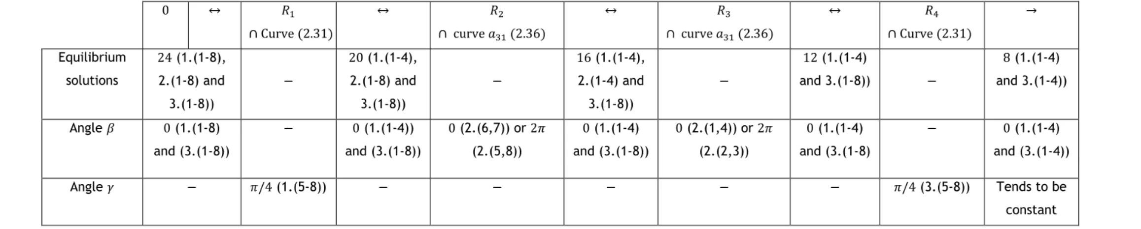
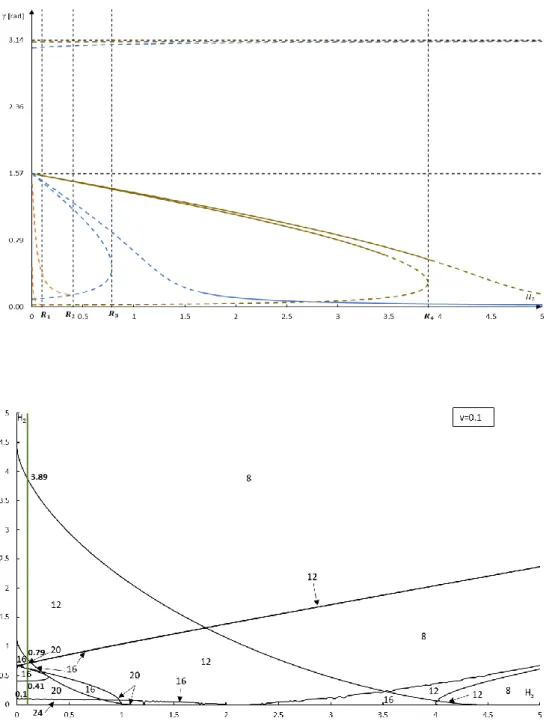
Figure 3.21 – Equilibria Picture for 𝑣𝐿= 0.1 and 𝐻3= 0.4 [14] ... 48

Figure 3.22 – Equilibria Picture for 𝑣𝐿= 0.1 and 𝐻3= 3.61 [14] ... 48

Figure 3.23 – Gyrostat’s equilibria bifurcation at 𝑣 = 0.11 with straight lines 𝐻3= 0.4 and 𝐻3= 3.61 ... 48

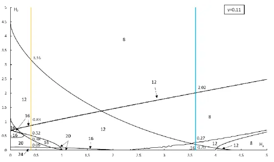
Figure 3.24 – Equilibria Picture for 𝑣𝐿= 0.25 and 𝐻3= 0.4 [14]... 49

Figure 3.25 – Equilibria Picture for 𝑣𝐿= 0.25 and 𝐻3= 3.264 [14] ... 49

Figure 3.26 – Gyrostat’s equilibria bifurcation at 𝑣 = 0.25 with straight lines 𝐻3= 0.4 and 𝐻3= 3.264... 49

xii

Figure 3.28 – Equilibria Picture for 𝑣𝐿= 0.6 and 𝐻3= 3.08 [14] ... 50 Figure 3.29 – Gyrostat’s equilibria bifurcation at 𝑣 = 0.6 with straight lines 𝐻3= 0.4 and 𝐻3= 3.08 ... 50 Figure 3.30 – Stability in function of angle 𝛾 and 𝐻2 and respective equilibria chart for 𝑣 = 0.1 and 𝐻3= 0.1 ... 53 Figure 3.31 – Stability in function of angle 𝛾 and 𝐻2 and respective equilibria chart for 𝑣 = 0.1 and 𝐻3= 2 ... 54 Figure 3.32 – Stability in function of angle 𝛾 and 𝐻2 and respective equilibria chart for 𝑣 = 0.1 and 𝐻3= 3.5 ... 55 Figure 3.33 – Stability in function of angle 𝛾 and 𝐻2 and respective equilibria chart for 𝑣 = 0.5 and 𝐻3= 0.1 ... 56 Figure 3.34 – Stability in function of angle 𝛾 and 𝐻2 and respective equilibria chart for 𝑣 = 0.5 and 𝐻3= 2 ... 57 Figure 3.35 – Stability in function of angle 𝛾 and 𝐻2 and respective equilibria chart for 𝑣 = 0.5 and 𝐻3= 5 ... 58 Figure 3.36 – Stability in function of angle 𝛾 and 𝐻2 and respective equilibria chart for 𝑣 = 1.0 and 𝐻3= 0.1 ... 59 Figure 3.37 – Stability in function of angle 𝛾 and 𝐻2 and respective equilibria chart for 𝑣 = 1.0 and 𝐻3= 2 ... 60 Figure 3.38 – Stability in function of angle 𝛾 and 𝐻2 and respective equilibria chart for 𝑣 = 1.0 and 𝐻3= 6 ... 61 Figure 3.39 – Stability in function of angle 𝛾 and 𝐻2 and respective equilibria chart for 𝑣 = 1.5 and 𝐻3= 0.1 ... 62 Figure 3.40 – Stability in function of angle 𝛾 and 𝐻2 and respective equilibria chart for 𝑣 = 1.5 and 𝐻3= 2 ... 63 Figure 3.41 – Stability in function of angle 𝛾 and 𝐻2 and respective equilibria chart for 𝑣 = 1.5 and 𝐻3= 10 ... 64 Figure 3.42 – Stability in function of angle 𝛾 and 𝐻2 and respective equilibria chart for 𝑣 = 5 and 𝐻3= 0.1 ... 65 Figure 3.43 – Stability in function of angle 𝛾 and 𝐻2 and respective equilibria chart for 𝑣 = 5 and 𝐻3= 2 ... 66 Figure 3.44 – Stability in function of angle 𝛾 and 𝐻2 and respective equilibria chart for 𝑣 = 5 and 𝐻3= 10 ... 67 Figure 3.45 – Stability in function of angle 𝛾 and 𝐻2 and respective equilibria chart for 𝑣 = 10 and 𝐻3= 0.1 ... 68 Figure 3.46 – Stability in function of angle 𝛾 and 𝐻2 and respective equilibria chart for 𝑣 = 10 and 𝐻3= 2 ... 69 Figure 3.47 – Stability in function of angle 𝛾 and 𝐻2 and respective equilibria chart for 𝑣 = 10 and 𝐻3= 10 ... 70

List of Tables

Table 3.1 – Color notation of Figure 3.6 ... 33 Table 3.2 – Equilibrium positions indexes for solutions of Group I, II and III ... 34 Table 3.3 – Summary of equilibrium solutions and spacecraft angles β and γ from Figure 3.8 ... 37

Nomenclature

𝑂: Gyrostat Center of Mass.

𝑂𝑋1𝑋2𝑋3: Orbital Reference Frame.

𝑂𝑋1: Axis aligned with the orbital plane, with positive direction in the direction of speed. 𝑂𝑋2: Axis normal to the orbital plane.

𝑂𝑋3: Axis that connects the center of mass of the planet with center of mass of the gyrostat. 𝑂𝑥1𝑥2𝑥3: Gyrostat’s fixed reference frame.

𝑂𝑥𝑖 (𝑖 = 1,2,3): Gyrostat’s principal axes of inertia.

𝛼, 𝛽 and 𝛾: the spacecraft angles between the gyrostat’s fixed reference frame and orbital reference frame.

𝑎𝑖𝑗: direction cosines between the principal axis and gyrostat axis.

𝐴, 𝐵 and 𝐶: principal moments of inertia in relation to the gyrostat’s center of inertia. 𝑝, 𝑞 and 𝑟: absolute angular velocity of the gyrostat.

ℎ̅ (𝑖 = 1, 2, 3): projections of the gyrostatic moment vector onto axes 𝑂𝑥𝑖 𝑖.

𝜔0: angular velocity of motion of the gyrostat’s center of mass along the circular orbit. 𝐻: Hamiltonian.

Chapter 1

Introduction

Artificial satellites are one of the most crucial components of modern life. Communications satellites lets billions of people connect with each other all over the world. The Global Positioning System (GPS) satellites constellation gives geolocation and time information to a GPS receiver leading to many civilian and military applications, such as accurate real-time navigation, clock synchronization, target tracking, among others. Meteorological satellites give us information about Earth’s environment. Finally, there are the scientific satellites, they allow scientists to study Earth, the solar system and even our universe in great detail and accuracy. These types of satellites have two big advantages compared to Earth-based solutions, like radio and optical telescopes: (a) observing celestial objects without the interference of gases, lights and magnetic fields produced on earth and (b) orbiting around other celestial objects, like sun, moon and other planets.

The attitude control and stabilization of an artificial satellite needs to be studied to ensure a successful operation, for example, in the case of a GPS satellite, its antenna must be pointing towards Earth. There are many methodologies that can be used in this case and they can be separated in two categories: passive methods can employ properties of the gravitational and magnetic fields, atmospheric drag, solar radiation pressure and gyroscopic properties of rotating bodies; and active methods, more accurate than the passive ones, using reaction wheels, thrusters and/or magnetic torques. Passive orientation systems own an important advantage comparing with active ones, as they can operate for a long time without energy and(or) a working body, and the last ones have a limited quantity of fuel and(or) need to ensure the reliability of the flywheels.

The motivating problem considered in this dissertation is the dynamics of the rotational motion of an artificial satellite, namely the gyrostat satellite family, in a circular orbit. This satellite is subjected to a gravitational torque and is equipped with internal rotors, as a semi-passive attitude stabilization. The internal rotors rotate at constant angular velocity relative to the satellite body and the gyrostatic moment vector lies along the Principal Plane of Inertia (𝐻1= 0) leading to new equilibrium positions that can be interesting in practical applications.

2

1.1 Important Concepts

In this section, it is introduced three important concepts related to the current work, which are: the gyrostat satellite, the relative equilibria of a gyrostat satellite and the Lyapunov’s stability of a gyrostat satellite.

A gyrostat satellite is mechanical system composed of a rigid body with one or more symmetrical rotors, whose spin axes are fixed in the rigid body and which can rotate about their axes of symmetry; it is also a satellite that is in orbit about a massive body. The gyrostat does not model several effects including flexible structures, bearing friction and dynamic and static imbalance. An example of a gyrostat motion in a circular orbit is given in figure 1.1.

Figure 1.1 – Gyrostat’s orbital scheme [1].

The relative equilibria of a gyrostat satellite is when the satellite rotates about the normal vector of the gyrostat’s orbital plane at the orbital rate, in a motionless way with respect to an observer in an orbit-fixed reference frame.

The Lyapunov’s stability of a gyrostat satellite is when the satellite motion remains always within a specific interval, i.e., an equilibrium position is stable when in reaction to small disturbances, there is small changes in its state of motion. The method used is the second method of Lyapunov, which makes use of a constant Lyapunov’s function. In this case, the system is stable when the Lyapunov’s matrix is positive definite and if a Lyapunov’s function is not dependent from time, it can be said that it remains time-invariant.

1.2 Literature Review

Since the ending of the 20th _{century until now, a widespread of studies in Celestial Mechanics} were conducted about the problems of gyrostat-satellites and its dynamics. The problem of controlling the motion of this type of rigid body with either internal or external torques was one of them. Among several studies, this dissertation has focused in gyrostat satellites with internal rotors attached to their principal axes of inertia. Exists two types of internal rotors applied to gyrostat satellites platforms, with freely spinning rotors and with constant-spin rotors.

The focus of this work is not on the case of freely spinning rotors but is important to have a wide view about the subject, so in 1998, El-Gohary [2], one relevant author, studied successfully how to reach asymptotic stability of relative programmed motion of a gyrostat-satellite using control moments applied on three internal rotors attached to its principal axes of inertia. In another study [3], the problem of exponential stability of the permanent rotational motion of a gyrostat satellite was investigated, but now stabilizing servo-control moments were applied to internal rotors. The equations of motion in this study are used without any approximations and the servo-control moments are obtained exactly. The same author in 2000 [4] proposed a control scheme that guarantee an optimal stabilization of a given rotational motion of a symmetric gyrostat on circular orbit. The control action is generated by rotating internal rotors. The asymptotic stability of this motion is proved using Barbachen and Krasovskii theorem and, as a particular case, for the equilibrium position of the gyrostat. In [5], a new control scheme is proposed for a gyrostat satellite, but in comparison with previous studies, this one has the advantage of choosing the time needed for stabilizing an arbitrary position to an equilibrium position.

For the next decade, the interest in dynamics of a gyrostat satellite moving along a circular orbit with constant speed rotors led to studies focused in different orientations of the vector of gyrostatic moment: in 2001, Sarychev and Mirer [6], show the special case when the vector of gyrostatic moment is collinear to the principal axis of inertia of the gyrostat and obtained a new analytical solution for equilibria. The authors concluded that the number of isolated equilibria is shown to be no less than 8 and no more than 24. Afterwards, in 2005, Sarychev et al. [7] investigated the same case but now shows the evolution of the regions of validity of the conditions of stability of the gyrostat and all bifurcation values of the parameters when these regions changes were obtained. In 2008, the same authors, focused their work in a different special case [8], when a gyrostatic moment vector lies on one of the satellite’s principal central planes of inertia. For this case, the equilibria were determined, and conditions of their existence were analyzed. A numerical-analytical method was used to study the evolution of the regions where the number of equilibria positions changes and to study the regions of validity of

4

gyrostat satellite in circular orbit around a spherical planet or with a symmetry axis [9], and the problem of stabilization of a rigid body motion with internal friction rotors, achieving new control laws.

In recent years, there was a change of focus and several authors start to discuss the general case of equilibria and stability of a gyrostat satellite subjected to gravitational torque, i.e. when all gyrostatic moment vector’s parameters are non-zero. The knowledge about the special cases [6], [7] and [8] added to new improvements in numerical computation led to deeper analysis of this case. The most relevant authors were Sarychev et al. In 2012 [10], it was determined the equilibria of a gyrostat satellite and was shown the number of equilibria is not less than 8 and no more than 24, like in previous cases. A year after [11], the same authors confirmed that for the same case the number of stable equilibria changes from 4 to 2 with increasing of the gyrostatic torque. A new symbolic-numerical method of computer algebra was proposed, in 2014, to study equilibrium positions of a gyrostat satellite [12-13]. The method uses an algorithm of constructing the Groebner bases and it results in a conversion of the system of 9 equations of 9 variables into a single algebraic equation of the 12th _{order with one variable.} This study reconfirms the same conclusions of previous studies about the maximum and minimum number of equilibria positions of gyrostat satellite.

In 2015, Luís Santos conducted a deep analysis into the dynamics of a gyrostat satellite in a circular orbit [14-15], specifically the general case of equilibria and stability. The author used the concepts and knowledge from [10-13], like the symbolic-numerical method from [12], which led to a vastly number of equilibria and stability configuration analysis, also unveiling the complete bifurcation of equilibria. In addition, it led to a deep understanding of the equilibria’s bifurcation curves, which corresponds to changes in number of equilibrium positions and to the study of its stability. This work unveiled small regions of 16 and 12 equilibrium positions near 𝐻1= 0, which up to date were unknown; these conclusions will be analyzed later in the present study. Henceforward, the conclusions of this study were reconfirmed in [16-17].

In [18], Gutnik and Sarychev investigated the proprieties of a non-linear algebraic system that determines equilibria of a gyrostat satellite. It is proposed a computer algebra method similar to last studies, which converts a very complex system into a simpler one. The focus of this work was when the gyrostatic moment vector lies in one of the satellite’s principal central planes of inertia (Case 𝐻1= 0, 𝐻2 and 𝐻3 non-zero; Case 𝐻2= 0, 𝐻1 and 𝐻3 non-zero; Case 𝐻3= 0, 𝐻1 and 𝐻2 non-zero). Equilibria and the bifurcation curves were all obtained symbolically. It is again reconfirmed for this cases that the number of equilibria ranges from 24 to 8 with decrement of 4 upon successive increase of the vector of gyrostatic moment.

Lastly, in 2017, a particular case (𝐻1= 0, 𝐻2 and 𝐻3 non-zero) [19] of equilibria of an asymmetrical inertial distribution gyrostat satellite was studied using the same symbolical-numerical method previously referred in [14]. The bifurcation curves in function of system

dimensionless parameters at which there was a change in number of equilibrium positions were determined. The study confirmed the existence of the small equilibria regions near 𝐻1= 0 shown on the general case of equilibria in [14] and [20]. In this dissertation, this special case will be analyzed furtherly.

1.3 Objectives

Many authors discussed the problem of attitude dynamics of a gyrostat satellite with constant spin-rate internal rotors, in different inertial distributions and different orientations of the gyrostatic moment vector. It was found in [14] and [20], small regions of 12 and 16 positions of equilibria which appear when one of component of gyrostatic moment vector is near zero (𝐻1≈ 0). Similarly, there are many studies about equilibria and stability of a gyrostat satellite when the gyrostatic moment vector lies in one of the satellite’s principal central planes of inertia (𝐻1≠ 0, 𝐻2= 0, 𝐻3≠ 0) in [8] and [18]; or when it is parallel to one of the satellite’s principal central axes of inertia (𝐻1= 0, 𝐻2≠ 0, 𝐻3= 0) in [6], [7] and [18]; but there are no published results when 𝐻1= 0, 𝐻2≠ 0, 𝐻3≠ 0.

This dissertation has the objective of providing a detail equilibria and stability study of a gyrostat satellite when the gyrostatic moment vector is along the principal plane of inertia (𝐻1= 0, 𝐻2≠ 0, 𝐻3≠ 0) using an analytical-numerical method. The study will be in function of a dimensionless inertia parameter and dimensionless gyrostatic moment vector components. To verify the appearance of the regions spoken above and for comparing purposes with [8], the complete bifurcation of equilibria with the bifurcation curves will be obtained and discussed. The evolution of the regions where sufficient conditions of stability is valid will be also investigated.

1.4 Dissertation overview

The present work is organized in five chapters: Introduction, Gyrostat’s Dynamics, Results and Discussion, and Conclusions and Future Work.

Chapter 2 develops an analytical-numerical approach to the mathematical problem of determining the equilibria and stability of the gyrostat satellite. All the equilibrium positions and the conditions of their existence are determined. The bifurcation curves equations and the sufficient conditions of stability of equilibria are also derived. The chapter also sets the assumptions, nomenclature and conventions used throughout the dissertation.

Chapter 3 discusses the results of equilibria and stability, in function of system parameters 𝑣, 𝐻2 and 𝐻3, obtained using the mathematical model. The evolution of equilibria bifurcation is discussed, as the evolution of stability of each equilibrium positions.

6

For the final chapter – Chapter 4 – it is presented the main conclusions and results, but also discusses recommendations, in which the study can be continued.

Chapter 2

Gyrostat’s Dynamics

In this chapter, a mathematical model based on a numerical-analytical approach for the calculation of the equilibrium positions and the sufficient conditions of stability of the gyrostat satellite is described. The equations of motion and conditions of existence of equilibrium for the gyrostat are obtained.

2.1 Equations of motion

This section describes the equations of motion that rules a solid body with rotors inside that are balanced both statically and dynamically. It is assumed the angular velocity of rotation of these rotors to be constant relative to the satellite’s main body, while the center of mass of the satellite moves along a circular orbit in a central Newtonian field of force.

It is introduced two right-handed Cartesian reference frames with an origin at the satellite’s center of mass 𝑂. 𝑂𝑋1𝑋2𝑋3 is the orbital reference frame whose axis 𝑂𝑋3 is directed along the radius vector connecting the center of mass of the satellite and the Earth; the 𝑂𝑋1 axis is directed along the linear velocity of the center of mass 𝑂.𝑂𝑥1𝑥2𝑥3 is the satellite-fixed reference frame; 𝑂𝑥𝑖 (𝑖 = 1, 2, 3) are the satellite’s principal axes of inertia.

8

Let’s us define the orientation of the satellite-fixed reference frame relative to the orbital reference frame by the spacecraft angles 𝛼, 𝛽 and 𝛾 represented in Figure 2.1, consequently, the direction cosines 𝑎𝑖𝑗 = cos(𝑋𝑖, 𝑥𝑗) are specified by the following expressions [8]:

{ 𝑎11= 𝑐𝑜𝑠𝛼 × 𝑐𝑜𝑠𝛽 𝑎12= 𝑠𝑖𝑛𝛼 × 𝑠𝑖𝑛𝛾 − 𝑐𝑜𝑠𝛼 × 𝑠𝑖𝑛𝛽 × 𝑐𝑜𝑠𝛾 𝑎13= 𝑠𝑖𝑛𝛼 × 𝑐𝑜𝑠𝛾 + 𝑐𝑜𝑠𝛼 × 𝑠𝑖𝑛𝛽 × 𝑠𝑖𝑛𝛾 𝑎21= 𝑠𝑖𝑛𝛽 𝑎22= 𝑐𝑜𝑠𝛽 × 𝑐𝑜𝑠𝛾 𝑎23= −𝑐𝑜𝑠𝛽 × 𝑠𝑖𝑛𝛾 𝑎31= −𝑠𝑖𝑛𝛼 × 𝑐𝑜𝑠𝛽 𝑎32= 𝑐𝑜𝑠𝛼 × 𝑠𝑖𝑛𝛾 + 𝑠𝑖𝑛𝛼 × 𝑠𝑖𝑛𝛽 × 𝑐𝑜𝑠𝛾 𝑎33= 𝑐𝑜𝑠𝛼 × 𝑐𝑜𝑠𝛾 − 𝑠𝑖𝑛𝛼 × 𝑠𝑖𝑛𝛽 × 𝑠𝑖𝑛𝛾 (2.1)

The spacecraft angles 𝛼, 𝛽 and 𝛾 can be written in function of the above direction cosines as:

{ 𝛼 = cos−1_(𝑎 11⁄𝑐𝑜𝑠𝛽) 𝛽 = sin−1_(𝑎 21) 𝛾 = cos−1_(𝑎 22⁄𝑐𝑜𝑠𝛽) (2.2)

The equations of motion of a gyrostat satellite with respect to its center of mass are written in the form [6,8-19]: { 𝐴𝑝̇ + (𝐶 − 𝐵)𝑞𝑟 − 3𝜔02(𝐶 − 𝐵)𝑎32𝑎33− ℎ̅̅̅𝑟 + ℎ2 ̅̅̅𝑞 = 03 𝐵𝑞̇ + (𝐴 − 𝐶)𝑟𝑝 − 3𝜔02(𝐴 − 𝐶)𝑎33𝑎31− ℎ̅̅̅𝑝 + ℎ3 ̅̅̅𝑟 = 01 𝐶𝑟̇ + (𝐵 − 𝐴)𝑝𝑞 − 3𝜔02(𝐵 − 𝐴)𝑎31𝑎32− ℎ̅̅̅𝑞 + ℎ1 ̅̅̅𝑝 = 02 (2.3) { 𝑝 = (𝛼̇ + 𝜔0)𝑎21+ 𝛾̇ = 𝑝̅ + 𝜔0𝑎21 𝑞 = (𝛼̇ + 𝜔0)𝑎22+ 𝛽̇𝑠𝑖𝑛𝛾 = 𝑞̅ + 𝜔0𝑎22 𝑟 = (𝛼̇ + 𝜔0)𝑎23+ 𝛽̇𝑐𝑜𝑠𝛾 = 𝑟̅ + 𝜔0𝑎23 (2.4)

Here, 𝐴, 𝐵, 𝐶 are the principal central moments of inertia of the gyrostat; 𝑝, 𝑞, 𝑟 are the absolute angular velocity of the gyrostat and ℎ̅ (𝑖 = 1, 2, 3) the projections of the gyrostatic 𝑖 moment vector onto axes 𝑂𝑥𝑖; and 𝜔0 is the angular velocity of motion of the gyrostat center of mass along the circular orbit. The dots designate differentiation with respect to time.

2.2 Gyrostat’s equilibria

Following [8] and others, for comparing reasons, it is used the same designations and parameters. First, it is introduced the designation ℎ̅ /𝜔𝑖 0= ℎ𝑖 and the following system of equations is obtained: { 4(𝐴𝑎21𝑎31+ 𝐵𝑎22𝑎32+ 𝐶𝑎23𝑎33) + ℎ1𝑎31+ ℎ2𝑎32+ ℎ3𝑎33= 0 𝐴𝑎11𝑎31+ 𝐵𝑎12𝑎32+ 𝐶𝑎13𝑎33= 0 𝐴𝑎11𝑎21+ 𝐵𝑎12𝑎22+ 𝐶𝑎13𝑎23+ ℎ1𝑎11+ ℎ2𝑎12+ ℎ3𝑎13= 0 (2.5)

This system allows one to determine all equilibrium positions of the gyrostat in the orbital reference frame.

In this case, 𝑎𝑖𝑗, as elements of an orthogonal matrix, satisfy the following conditions:

{ 𝑎112 + 𝑎122 + 𝑎132 = 1 𝑎212 + 𝑎222 + 𝑎232 = 1 𝑎312 + 𝑎322 + 𝑎332 = 1 𝑎11𝑎21+ 𝑎12𝑎22+ 𝑎13𝑎23= 0 𝑎11𝑎31+ 𝑎12𝑎32+ 𝑎13𝑎33= 0 𝑎21𝑎31+ 𝑎22𝑎32+ 𝑎23𝑎33= 0 (2.6)

At 𝐴 ≠ 𝐵 ≠ 𝐶 one can solve system (2.5) and (2.6) for 𝑎11, 𝑎12, 𝑎13, 𝑎21, 𝑎22, 𝑎23 and 𝑎23. As a result, we get [8]: { 𝑎11= 4(𝐶 − 𝐵)𝑎32𝑎33 𝐹 𝑎12= 4(𝐴 − 𝐶)𝑎33𝑎31 𝐹 𝑎13= 4(𝐵 − 𝐴)𝑎31𝑎32 𝐹 𝑎21= 4(𝐼3− 𝐴)𝑎31 𝐹 𝑎22= 4(𝐼3− 𝐵)𝑎32 𝐹 𝑎23= 4(𝐼3− 𝐶)𝑎33 𝐹 (2.7)

Here, 𝐹 = ℎ1𝑎31+ ℎ2𝑎32+ ℎ3𝑎33, 𝐼3= 𝐴𝑎312 + 𝐵𝑎322 + 𝐶𝑎332 and direction cosines 𝑎31, 𝑎32 and 𝑎33 are determined from the following three equations:

10 16[(𝐵 − 𝐶)2_𝑎 32 2 _𝑎 33 2 _{+ (𝐶 − 𝐴)}2_𝑎 33 2 _𝑎 312 + (𝐴 − 𝐵)2𝑎312 𝑎322 ] = (ℎ1𝑎31+ ℎ2𝑎32+ ℎ3𝑎33)2 4(𝐵 − 𝐶)(𝐶 − 𝐴)(𝐴 − 𝐵)𝑎31𝑎32𝑎33+ [ℎ1(𝐵 − 𝐶)𝑎32𝑎33+ ℎ2(𝐶 − 𝐴)𝑎33𝑎31+ ℎ3(𝐴 − 𝐵) × 𝑎31𝑎32] × (ℎ1𝑎31+ ℎ2𝑎32+ ℎ3𝑎33) = 0 (2.8) 𝑎312 + 𝑎322 + 𝑎332 = 1

After solving system (2.8) formulas (2.7) allow one to determine the remaining six direction cosines. Notice that solutions (2.7) exist only when out of three direction cosines 𝑎31, 𝑎32 and 𝑎33, none two vanish simultaneously. The cases 𝑎31= 𝑎32= 0, 𝑎32= 𝑎33= 0 and 𝑎33= 𝑎31= 0 are special and they should be considered immediately addressing to system (2.5) and (2.6). The case 𝑎32= 𝑎33= 0 will be discussed later.

2.2.1 Case 𝑯

= 𝟎, 𝑯

≠ 𝟎 and 𝑯

≠ 𝟎

In previous studies, it is analyzed the general case of the gyrostat (𝐻1≠ 0, 𝐻2≠ 0 and 𝐻3≠ 0) [14] and many particular cases, the case when the gyrostatic moment vector is collinear to one of the satellite’s principal central axes of inertia (𝐻1= 0, 𝐻2≠ 0 and 𝐻3= 0) [6] and the case when the gyrostatic moment vector is parallel to the satellite’s principal central planes of inertia (𝐻1≠ 0, 𝐻2= 0 and 𝐻3≠ 0) [8]. In this study, we deepen the knowledge about the case when the gyrostatic moment vector is along the satellite’s principal central plane of inertia, which parameter 𝐻1 is zero (𝐻1= 0, 𝐻2≠ 0 and 𝐻3≠ 0).

The system (2.8) after introducing the dimensionless parameters:

𝐻2= ℎ2 𝐶 − 𝐴 𝐻3= ℎ3 𝐶 − 𝐴 𝑣 = 𝐴 − 𝐵 𝐶 − 𝐴 (2.9) Takes on form: { 16[𝑎322 𝑎332 (𝑣 + 1)2+ 𝑎312 𝑎332 + 𝑎231𝑎322 𝑣2] = (𝐻2𝑎32+ 𝐻3𝑎33)2 𝑎31{−4𝑣(1 + 𝑣)𝑎32𝑎33+ [𝐻2𝑎33+ 𝐻3𝑎32𝑣] × (𝐻2𝑎32+ 𝐻3𝑎33)} = 0 𝑎312 + 𝑎322 + 𝑎332 = 1 (2.10)

Notice that the dimensionless parameters 𝑣, being an inertial parameter of the satellite, does not in itself determine the shape of its ellipsoid of inertia.

When investigating system (2.10) it is necessary to consider three cases: (𝑎31= 0, 𝑎32≠ 0 and 𝑎33≠ 0), (𝑎31≠ 0 and 𝑎32 = 𝑎33= 0) and (𝑎31≠ 0, 𝑎32≠ 0 and 𝑎33≠ 0).

2.2.1.1 Case 𝒂

≠ 𝟎 and 𝒂

= 𝒂

= 𝟎

The following system takes on the form:

{

16[𝑎322 𝑎332 (𝑣 + 1)2+ 𝑎312 𝑎332 + 𝑎312 𝑎322 𝑣2] = (𝐻2𝑎32+ 𝐻3𝑎33)2 −4𝑣(1 + 𝑣)𝑎32𝑎33+ [𝐻2𝑎33+ 𝐻3𝑎32𝑣] × (𝐻2𝑎32+ 𝐻3𝑎33) = 0 𝑎312 + 𝑎322 + 𝑎332 = 1

(2.11)

From the second equation of system (2.11) it follows that, if 𝑎32= 0, then also 𝑎33= 0. The existence of a solution for which:

𝑎32= 𝑎33= 0 (2.12)

It is investigated by analyzing original equations (2.5) and (2.6):

{ 4𝐴𝑎21𝑎31= 0 𝐴𝑎11𝑎31= 0 𝐴𝑎11𝑎21+ 𝐵𝑎12𝑎22+ 𝐶𝑎13𝑎23+ ℎ2𝑎12+ ℎ3𝑎13= 0 ⇔ ⇔ { 𝑎21= 0 𝑎11= 0 𝐵𝑎12𝑎22+ 𝐶𝑎13𝑎23+ ℎ2𝑎12+ ℎ3𝑎13= 0 (2.13) { 𝑎122 + 𝑎132 = 1 𝑎222 + 𝑎232 = 1 𝑎312 = 1 (2.14) { 𝑎12𝑎22+ 𝑎13𝑎23= 0 0 = 0 0 = 0 (2.15)

In this case, equations (2.5) after conversion to dimensionless parameters (2.9) and orthogonality (2.6) leads to the system:

{(𝐵 − 𝐶)𝑎12𝑎22+ ℎ2𝑎12+ ℎ3𝑎13= 0 𝑎12𝑎22= −𝑎12𝑎22

⟺

⇔ {−(1 + 𝑣)𝑎12𝑎22+ 𝐻2𝑎12+ 𝐻3𝑎13= 0

12

In summary, the system becomes:

{ −(1 + 𝑣)𝑎12𝑎22+ 𝐻2𝑎12+ 𝐻3𝑎13= 0 𝑎312 = 1 𝑎11= 0 𝑎21= 0 𝑎122 + 𝑎132 = 1 𝑎222 + 𝑎232 = 1 𝑎12𝑎22+ 𝑎13𝑎23= 0 (2.17)

Analyzing the first equation of this system, we obtain:

−(1 + 𝑣)𝑎12𝑎22+ 𝐻2𝑎12+ 𝐻3𝑎13= 0 ⇔ ⇔ 𝑎12(𝐻2− 𝑎22(𝑣 + 1)) + 𝐻3𝑎13= 0 ⇔ ⇔ 𝑎12= − 𝐻3𝑎13 𝐻2− 𝑎22(𝑣 + 1) (2.18)

From the last equation of system (2.17) and the expression for 𝑎12 obtained above (2.18), it can be achieved the following relationship:

𝑎12𝑎22+ 𝑎13𝑎23= 0 ⇔ ⇔ 𝑎12= − 𝑎13𝑎23 𝑎22 ⇔ ⇔ − 𝐻3𝑎13 𝐻2− 𝑎22(1 + 𝑣) = −𝑎13𝑎23 𝑎22 ⇔ ⇔𝑎23 𝑎22 = 𝐻3 𝐻2− 𝑎22(𝑣 + 1) (2.19)

Introducing 𝑎232 = 1 − 𝑎222 and raising the previous relationship to the power 2, it is obtained an equation of fourth order in 𝑥1= 𝑎22:

(𝑎23 𝑥1 ) 2 = ( 𝐻3 𝐻2− 𝑥1(𝑣 + 1) ) 2 ⇔ ⇔1 − 𝑥1 2 𝑥12 = 𝐻3 2 (𝐻2− 𝑥1(𝑣 + 1)) 2⇔ ⇔ −(𝑣 + 1)2_𝑥 14+ 2𝐻2(𝑣 + 1)𝑥13+ ((𝑣 + 1)2− 𝐻32− 𝐻22)𝑥12− 2𝐻2(𝑣 + 1)𝑥1+ 𝐻22= 0 (2.20)

Two equilibrium positions of the gyrostat correspond to each real root of this equation. The direction cosines are defined in function of 𝑥1:

𝑎12= − 𝑎13𝑎23 𝑎22 (2.21) 𝑎12𝑎22+ 𝑎13𝑎23= 0 ⇔ ⇔ −𝐻3𝑎13𝑥1 𝐻2− 𝑥1(𝑣 + 1) + 𝑎13𝑎23= 0 ⇔ ⇔ 𝑎23= 𝐻3𝑥1 𝐻2− 𝑥1(𝑣 + 1) (2.22)

Using the 5th _{equation of (2.17) and equation (2.21), it is achieved:} 𝑎232 𝑎132 𝑥₁2 + 𝑎132 = 1 ⇔ ⇔ 𝑎232 𝑎132 + 𝑎132 𝑥12= 𝑥12⇔ ⇔ 𝑎132 (𝑥12+ 𝑎232 ) = 𝑥12⇔ ⇔ 𝑎132 = 𝑥12⇔ ⇔ 𝑎13= 𝑎31𝑥1 (2.23) 𝑎12= − 𝑎23 𝑥1 𝑎13⇔ ⇔ 𝑎12= − 𝑎23 𝑥1 𝑎31𝑥1⇔ ⇔ 𝑎12= −𝑎23𝑎31 (2.24)

14

Together, they form the group of solutions I:

{ 𝑎11= 0 𝑎12= −𝑎23𝑎31 𝑎13= 𝑎31𝑥1 𝑎21= 0 𝑎22= 𝑥1 𝑎23= 𝐻3𝑥1 𝐻2− 𝑥1(𝑣 + 1) 𝑎31= ±1 𝑎32= 0 𝑎33= 0 (2.25)

Let us determine boundaries in the plane of the parameters 𝐻2 and 𝐻3 that separate domains with different numbers of solutions of system (2.17). Bifurcation points are points in the plane (𝐻2,𝐻3) that simultaneously belong to the hyperbola branch that does not pass through the origin and to the circle; the tangent lines to the hyperbola and the circle coincide at the bifurcation points. The condition that the tangent lines coincide has the form [18]:

𝑑(𝑎23) 𝑑(𝑎22) = 𝐻3(𝑣 + 1)𝑎22 (𝐻2− 𝑎22(𝑣 + 1)) 2+ 𝐻3 𝐻2− 𝑎22(𝑣 + 1) =(𝑣 + 1)𝑎23+ 𝐻3 𝐻2− 𝑎22(𝑣 + 1) = −𝑎22 𝑎23 ⇔ ⇔ (𝑣 + 1)(𝑎232 − 𝑎222 ) + 𝑎22𝐻2+ 𝑎23𝐻3= 0 (2.26) Substituting the expression for 𝑎23 from (2.25) into the sixth equation of (2.17) and equation (2.26), it is obtained the following system:

{ 𝑎222 + 𝑎232 = 1 𝑎23= 𝐻3𝑎22 𝐻2− 𝑎22(𝑣 + 1) ⇔ ⇔ { 𝐻32𝑎222 (𝐻2− 𝑎22(𝑣 + 1)) 2= 1 − 𝑎222 − (2.27) { (𝑣 + 1)(𝑎232 − 𝑎222 ) + 𝑎22𝐻2+ 𝑎23𝐻3= 0 𝑎23= 𝐻3𝑎22 𝐻2− 𝑎22(𝑣 + 1) ⇔ ⇔ {−𝑎222 (𝑣 + 1) + 𝑎222 𝐻32(𝑣 + 1) (𝐻2− 𝑎22(𝑣 + 1)) 2+ 𝑎22𝐻2+ 𝑎22𝐻32 𝐻2− 𝑎22(1 + 𝑣) = 0 − ⇔

⇔ 𝑎222 𝐻32(𝑣 + 1) − 𝑎222 (𝑣 + 1)(𝐻2− 𝑎22(1 + 𝑣)) 2 + 𝑎22𝐻2(𝐻2− 𝑎22(1 + 𝑣)) 2 + 𝑎22𝐻32(𝐻2− 𝑎22(𝑣 + 1)) = 0 ⇔ ⇔ 𝑎22(𝐻2− 𝑎22(𝑣 + 1)) 2 (𝐻2− 𝑎22(𝑣 + 1)) + 𝑎22𝐻32(𝑎22(𝑣 + 1) + (𝐻2− 𝑎22(1 + 𝑣)) = 0 ⇔ ⇔ 𝐻3 2_𝐻 2 (𝐻2− 𝑎22(𝑣 + 1)) 2= −(𝐻2− 𝑎22(1 + 𝑣)) (2.28) { 𝐻32𝑎222 (𝐻2− 𝑎22(𝑣 + 1)) 2= 1 − 𝑎222 𝐻32𝐻2 (𝐻2− 𝑎22(𝑣 + 1)) 2= −(𝐻2− 𝑎22(1 + 𝑣)) (2.29)

Dividing the first equation by the second equation from system (2.29), it is obtained: 𝐻32𝑎222 (𝐻2− 𝑎22(𝑣 + 1)) 2 𝐻32𝐻2 (𝐻2− 𝑎22(𝑣 + 1)) 2 = 1 − 𝑎22 2 −(𝐻2− 𝑎22(1 + 𝑣)) ⇔ ⇔𝑎22 2 𝐻2 = 1 − 𝑎22 2 −(𝐻2− 𝑎22(𝑣 + 1)) ⇔ ⇔ −𝑎222 𝐻2+ 𝑎223 (𝑣 + 1) = 𝐻2− 𝐻2𝑎222 ⇔ ⇔ 𝑎22= ( 𝐻2 𝑣 + 1) 1 3 ⁄ (2.30)

Ultimately, substituting the expression for 𝑎22 into the second equation (2.29), it is obtained the following astroid equation:

− 𝐻3 2_𝐻 2 (𝐻2− 𝑎22(𝑣 + 1)) 2= −(𝐻2− 𝑎22(𝑣 + 1)) ⇔ ⇔ 𝐻32𝐻2= (𝐻2− 𝑎22(𝑣 + 1)) 3 ⇔ ⇔ −𝐻₃2 3⁄ 𝐻₂1 3⁄ = 𝐻2− 𝑎22(𝑣 + 1) ⇔ ⇔ −𝐻3 2 3⁄ 𝐻2 1 3⁄ = 𝐻2 1 3⁄ 𝐻2 2 3⁄ − 𝐻2 1 3⁄ (𝑣 + 1)2 3⁄ ⇔ ⇔ 𝐻₂2 3⁄ + 𝐻₃2 3⁄ = (𝑣 + 1)2 3⁄ _(2.31)

16

Therefore, equation (2.20) has four roots at 𝐻₂2 3⁄

+ 𝐻₃2 3⁄ < (𝑣 + 1)2 3⁄ _{and two roots at 𝐻} 2 2 3⁄

+ 𝐻₃2 3⁄ > (𝑣 + 1)2 3⁄ _{. Consequently, the total number of equilibrium positions for case (2.12), i.e.,} the number of solutions of group I, can be either 8 or 4, depending on the relation between dimensionless parameters 𝐻2 and 𝐻3.

2.2.1.2 Case 𝒂

≠ 𝟎, 𝒂

≠ 𝟎 and 𝒂

≠ 𝟎

Let us consider system (2.11) at 𝑎32≠ 0 and 𝑎33≠ 0. Dividing the second equation of this system by 𝑎332 and designating 𝑥2= 𝑎32/𝑎33, it can be rewritten in the form:

−4𝑣(𝑣 + 1)𝑎32𝑎33+ 𝐻22𝑎32𝑎33+ 𝐻2𝐻3𝑎332 + 𝐻2𝐻3𝑣𝑎322 + 𝐻32𝑣𝑎32𝑎33= 0 ⇔ ⇔ − 4𝑣(𝑣 + 1)𝑎32⁄𝑎33+ 𝐻22𝑎32⁄𝑎33+ 𝐻2𝐻3+ 𝐻2𝐻3𝑣𝑎322 ⁄𝑎332 + 𝐻32𝑣𝑎32⁄𝑎33= 0 ⇔

⇔ 𝐻2𝐻3𝑣𝑥22+ (𝐻22+ 𝐻32𝑣 − 4𝑣(𝑣 + 1))𝑥2+ 𝐻2𝐻3= 0 (2.32) The solution to this equation has the form:

𝑥2= −(𝐻22+ 𝐻32𝑣 − 4𝑣(𝑣 + 1)) ± √Δ 2𝐻3𝐻2𝑣 (2.33) Where: Δ = (𝐻22+ 𝐻32𝑣 − 4𝑣(1 + 𝑣)) 2 − 4𝐻22𝐻32𝑣 (2.34)

The first and third equations of system (2.11) after substitution in them 𝑎32= 𝑥2𝑎33 leads to the following system:

{16[𝑥2 2_𝑎 334 (𝑣 + 1)2+ 𝑎312 𝑎332 + 𝑣2𝑥22𝑎312 𝑎332 ] = (𝐻2𝑎33𝑥2+ 𝐻3𝑎33)2 𝑎312 + 𝑎322 + 𝑎332 = 1 ⇔ ⇔ {16[𝑥2 2_𝑎 33 4 _{(𝑣 + 1)}2_{+ 𝑎} 312 𝑎332 + 𝑣2𝑥22𝑎312 𝑎332 ] = 𝑎332 (𝐻2𝑥2+ 𝐻3)2 − ⇔ ⇔ {𝑎332 𝑥22(𝑣 + 1)2+ 𝑎312 (1 + 𝑣2𝑥22) = (𝐻2𝑥2+ 𝐻3)2 16 − ⇔ ⇔ { − 𝑎312 + 𝑥22𝑎332 + 𝑎332 = 1 ⇔ ⇔ {𝑎332 𝑥22(𝑣 + 1)2+ 𝑎312 (1 + 𝑣2𝑥22) = (𝐻2𝑥2+ 𝐻3)2 16 𝑎332 (1 + 𝑥22) + 𝑎312 = 1 (2.35)

Resolving this system for 𝑎312 and 𝑎332 , it gets: { 𝑎312 = (𝐻3+ 𝐻2𝑥2)2(𝑥22+ 1) − 16𝑥22(𝑣 + 1)2 16(𝑣𝑥22− 1)2 𝑎332 = 16(𝑣2_𝑥 22+ 1) − (𝐻3+ 𝐻2𝑥2)2 16(𝑣𝑥22− 1)2 (2.36)

In order for the found solution would correspond to an equilibrium solution of the gyrostat, the conditions Δ ≥ 0, 𝑎312 ≥ 0 and 𝑎332 ≥ 0 must be met.

Let us consider the discriminant sign. It is clear that Δ ≥ 0 if 𝑣 ≤ 0. In order to determine the sign of Δ on the interval 𝑣 > 0, the discriminant can be written as:

Δ = [(𝐻3+ 2√𝑣 + 1) 2

𝑣 − 𝐻22] × [(𝐻3− 2√𝑣 + 1) 2

𝑣 − 𝐻22] (2.37)

Analyzing this expression, it can be concluded that Δ ≥ 0 at:

{(𝐻2+ 2√𝑣 + 1) 2 𝑣 ≥ 𝐻22 (𝐻2− 2√𝑣 + 1) 2 𝑣 ≥ 𝐻22 ∨ {(𝐻2+ 2√𝑣 + 1) 2 𝑣 ≤ 𝐻22 (𝐻2− 2√𝑣 + 1) 2 𝑣 ≤ 𝐻22 (2.38)

Now, the conditions 𝑎312 ≥ 0 and 𝑎332 ≥ 0 will be analyzed. Considering the following relationship obtained from the second equation of system (2.11)):

𝑥2+ 𝐻3=

4𝑣(𝑣 + 1)𝑥2 𝐻2+ 𝐻3𝑣𝑥2

(2.39)

And introducing that on (2.36), these conditions became: 𝑎312 ≥ 0 ⟺ ⟺(𝐻3+ 𝐻2𝑥2) 2_(𝑥 22+ 1) − 16𝑥22(𝑣 + 1)2 16(𝑣𝑥22− 1)2 ≥ 0 ⟺ ⇔ (𝐻3+ 𝐻2𝑥2)2(𝑥22+ 1) − 16𝑥22(𝑣 + 1)2≥ 0 ⇔ ⇔16𝑣 2_{(𝑣 + 1)}2_𝑥 22(𝑥22+ 1) (𝐻2+ 𝐻3𝑣𝑥2)2 − 16𝑥22(𝑣 + 1)2≥ 0 ⇔ ⇔16𝑣 2_𝑥 22(𝑣 + 1)2(𝑥22+ 1) − 16𝑥22(𝑣 + 1)2(𝐻2+ 𝐻3𝑣𝑥2)2 (𝐻2+ 𝐻3𝑣𝑥2)2 ≥ 0 ⇔ ⇔ 𝑣2_(𝑥 22+ 1) − (𝐻2+ 𝐻3𝑣𝑥2)2≥ 0 (2.40)

18 𝑎332 ≥ 0 ⇔ ⇔16(𝑣 2_𝑥 22+ 1) − (𝐻3+ 𝐻2𝑥2)2 16(𝑣𝑥₂2_{− 1)}2 ≥ 0 ⇔ ⇔ 16(𝑣2_𝑥 22+ 1) − (𝐻3+ 𝐻2𝑥2)2≥ 0 (2.41) In other way, the inequalities (2.40) and (2.41) can be grouped with the equation (2.32) forming the following system, similar to the one found in [8]:

{ 𝑎0𝑥2+ 𝑎1𝑥2+ 𝑎2≥ 0 𝑏0𝑥2+ 𝑏1𝑥2+ 𝑏2≥ 0 𝑐0𝑥22+ 𝑐1𝑥2+ 𝑐2= 0 ⇔ ⇔ { 𝑎0𝑥2+ 𝑎1𝑥2+ 𝑎2≥ 0 𝑏0𝑥2+ 𝑏1𝑥2+ 𝑏2≥ 0 𝑥2= −𝑐1± √𝑐12− 4𝑐0𝑐2 2𝑐0 ⇔ ⇔ { (−𝑐1± √𝑐12− 4𝑐0𝑐2) (𝑎1𝑐0− 𝑎0𝑐1) + 2𝑐0(𝑎2𝑐0− 𝑎0𝑐2) ≥ 0 (−𝑐1± √𝑐12− 4𝑐0𝑐2) (𝑏1𝑐0− 𝑏0𝑐1) + 2𝑐0(𝑏2𝑐0− 𝑏0𝑐2) ≥ 0 − (2.42) Where: { 𝑎0= 𝑣2(1 − 𝐻32) 𝑎1= −2𝐻2𝐻3𝑣 𝑎2= −𝐻22+ 𝑣2 { 𝑏0= 16𝑣2− 𝐻22 𝑏1= −2𝐻2𝐻3 𝑏2= 16 − 𝐻32 { 𝑐0= 𝐻2𝐻3𝑣 𝑐1= 𝐻22+ 𝐻32𝑣 − 4𝑣(𝑣 + 1) 𝑐2= 𝐻2𝐻3

A solution of system (2.11) only correspond to an equilibrium positions of a gyrostat when inequalities (2.42) and Δ = 𝑐12− 4𝑐0𝑐2≥ 0 are valid. In this case, 𝑎32= 𝑥2𝑎33, direction cosines 𝑎31 and 𝑎33 are determined from (2.36), and the remaining direction cosines, taking (2.7) and (2.9) into account, take on the form:

{ 𝑎11= 4𝑣𝑎32𝑎33 𝐻2𝑎32+ 𝐻3𝑎33 𝑎12= − 4𝑎31𝑎33 𝐻2𝑎32+ 𝐻3𝑎33 𝑎13= − 4𝑣𝑎31𝑎32 𝐻2𝑎32+ 𝐻3𝑎33 𝑎21= 4𝑎31 𝑎332 − 𝑣𝑎322 𝐻2𝑎32+ 𝐻3𝑎33 𝑎22= 4𝑎32 (𝑣 + 1)𝑎332 + 𝑣𝑎312 𝐻2𝑎32+ 𝐻3𝑎33 𝑎23= −4𝑎33 (𝑣 + 1)𝑎322 + 𝑎312 𝐻2𝑎32+ 𝐻3𝑎33 (2.43)

It can be concluded that in this case, the number of possible equilibrium positions, forming the group of solutions II, does not exceed 8.

2.2.1.3 Case 𝒂

= 𝟎, 𝒂

≠ 𝟎 and 𝒂

≠ 𝟎

At last, let us consider systems (2.5) and (2.6) which leads to:

{ 4(𝐵𝑎22𝑎32+ 𝐶𝑎23𝑎33) + ℎ2𝑎32+ ℎ3𝑎33= 0 0 = 0 0 = 0 (2.44) { 𝑎112 = 1 𝑎222 + 𝑎232 = 1 𝑎322 + 𝑎332 = 1 (2.45) { 𝑎21= 0 0 = 0 𝑎22𝑎32+ 𝑎23𝑎33= 0 (2.46)

Utilizing the first equation from (2.44) and the last equation from (2.46), we can obtain a 4th order equation in function of 𝑥3= 𝑎22:

𝑎22𝑎32+ 𝑎23𝑎33= 0 ⟺ ⟺ 𝑎32= − 𝑎23𝑎33 𝑎22 (2.47) 4(𝐵 − 𝐶)𝑎22𝑎32+ ℎ2𝑎32+ ℎ3𝑎33= 0 ⇔

20 ⇔ 𝑎32(𝐻2− 4(𝑣 + 1)𝑎22) + 𝐻3𝑎33= 0 ⇔ ⇔ 𝑎32= − 𝐻3𝑎33 𝐻2− 4(𝑣 + 1)𝑎22 ⇔ ⇔ −𝑎23𝑎33 𝑎22 = − 𝐻3𝑎33 𝐻2− 4(𝑣 + 1)𝑎22 ⇔ ⇔ (𝑎23 𝑎22 ) 2 = ( 𝐻3 𝐻2− 4(𝑣 + 1)𝑎22 ) 2 ⇔

Introducing 𝑎232 = 1 − 𝑎222 and raising the previous relationship to the power 2:

⇔1 − 𝑥3 2 𝑥32 = 𝐻3 2 (𝐻2− 4(𝑣 + 1)𝑥3)2 ⇔ ⇔ −16(𝑣 + 1)2_𝑥 34+ 8𝐻2(𝑣 + 1)𝑥33+ (−𝐻22− 𝐻32+ 16(𝑣 + 1)2)𝑥32− 8𝐻2(𝑣 + 1)𝑥3 + 𝐻22= 0 (2.48) Similar to first case (2.2.1.1), two equilibrium positions of the gyrostat correspond to each real root of this equation. The direction cosines are defined in function of 𝑥3:

𝑎22𝑎32+ 𝑎23𝑎33= 0 ⇔ ⇔ − −𝑥3𝐻3𝑎33 𝐻2− 4(𝑣 + 1)𝑥3 + 𝑎23𝑎33= 0 ⇔ ⇔ 𝑎23= 𝐻3𝑥3 𝐻2− 4(𝑣 + 1)𝑥3 (2.49) 𝑎232 𝑎332 𝑥32 + 𝑎332 = 1 ⇔ ⇔ 𝑎232 𝑎332 + 𝑎332 𝑥32= 𝑥32⇔ ⇔ 𝑎332 (𝑎232 + 𝑥32) = 𝑥32⇔ ⇔ 𝑎33= 𝑥3𝑎11 (2.50) 𝑎32= − 𝑎23𝑎11𝑥3 𝑥3 ⇔ ⇔ 𝑎32= −𝑎23𝑎11 (2.51)

Together, they form the group of solutions III: { 𝑎11= ±1 𝑎12= 0 𝑎13= 0 𝑎21= 0 𝑎22= 𝑥3 𝑎23= 𝐻3𝑥3 𝐻2− 4(𝑣 + 1)𝑥3 𝑎31= 0 𝑎32= −𝑎23𝑎11 𝑎33= 𝑥3𝑎11 (2.52)

Similarly to (2.20), the equation is of fourth order and can have either 4 or 2 real roots. The number of roots changes on the surface are determined, using the same method as in the case (2.2.1.1), by the equation:

𝐻₂2 3⁄ + 𝐻₃2 3⁄ = (4(𝑣 + 1))2 3⁄ (2.53)

Four roots exist at 𝐻₂2 3⁄ + 𝐻3

2 3⁄

< (4(𝑣 + 1))2 3⁄ and two roots at 𝐻2 2 3⁄

+ 𝐻3 2 3⁄

> (4(𝑣 + 1))2 3⁄ . Thus, the number of solutions of group III can be either 4 or 8.

2.3 Gyrostat’s stability

In this section, the Lyapunov’s stability theory is reviewed and the sufficient conditions of stability for the equilibrium positions of a gyrostat satellite are obtained.

Consider in this study a dynamical system which satisfies:

𝑥̇ = 𝑓(𝑥) 𝑥(𝑡𝑜) = 𝑥0 𝑥 ∈ ℝ𝑛 (2.54)

According to [21], it is assumed that 𝑓(𝑥) is Lipschitz continuous with respect to 𝑥 and uniformly in 𝑡. A point 𝑥∗_{∈ ℝ}𝑛 _{is an equilibrium position of (2.54) if 𝑓(𝑥}∗_{) = 0.}

The equilibrium position 𝑥∗ _{is stable in the sense of Lyapunov, if for any 𝜖 > 0 there exists a} 𝛿(𝜖) > 0 such that

‖𝑥(𝑡0)‖ < 𝛿 ⟹ ‖𝑥(𝑡)‖ < 𝜖, ∀𝑡 ≥ 0 (2.55) This definition of stability does not require that trajectories starting close to the origin tend to the origin asymptotically, in other words, the solutions which start in a neighborhood of 𝑥∗

22

The case of asymptotic stability is different, as solutions that are near an equilibrium position tend to the equilibrium position itself. In a mathematical way, the equilibrium position 𝑥∗ _is asymptotically stable if 𝑥∗ _{is stable in the sense of Lyapunov and 𝑥}∗ _{is attractive, i.e, there} exists 𝛿 such that:

‖𝑥(𝑡0)‖ < 0 ⟹ lim

𝑡⟶∞𝑥(𝑡) = 0 (2.56)

Figure 2.2 shows a comparison between stable and unstable equilibrium positions.

Figure 2.2 – Phase portraits for stable and unstable equilibrium positions [21]

There is another method developed by Lyapunov called Lyapunov’s direct method (or second method of Lyapunov). In the literature in general, the method is seen as the most reliable in the study of stability of aerospace guidance systems, which typically contain strong nonlinearities. The method assumes that the energy of a system can be measured, therefore can be defined as a Lyapunov’s function. The study of the rate of change of the energy of the system can ascertain the stability of an equilibrium position.

As in previous studies [8] and [14], the generalized energy integral is continuous, therefore it can be used as Lyapunov’s function:

1 2(𝐴𝑝̅ 2_{+ 𝐵𝑞}2_{+ 𝐶𝑟̅}2_{) +}3 2𝜔0 2_{[(𝐴 − 𝐶)𝑎} 31 2 _{+ (𝐵 − 𝐶)𝑎} 32 2 _{] +}1 2𝜔0 2_{[(𝐵 − 𝐴)𝑎} 21 2 _{+ (𝐵 − 𝐶)𝑎} 232 ] − 𝜔0[ℎ̅̅̅𝑎1 21+ ℎ̅̅̅𝑎2 22+ ℎ̅̅̅𝑎3 23] = 𝐻

Remembering the dimensionless parameters:

𝑣 =𝐴 − 𝐵 𝐶 − 𝐴 𝐻𝑖= ℎ𝑖 𝐶 − 𝐴 ℎ𝑖= ℎ̅𝑖 𝜔𝑜 (2.58) (2.57)

It can be deducted that: { ℎ𝑖= ℎ̅𝑖 𝜔0 𝐻𝑖= ℎ𝑖 𝐶 − 𝐴 ⟺ ⇔ {_ℎ − 𝑖= 𝐻𝑖(𝐶 − 𝐴) ⟺ ⇔ {𝐻𝑖(𝐶 − 𝐴) = ℎ̅𝑖 𝜔0 − ⟺ ⇔ {ℎ̅ = 𝜔𝑖 0𝐻𝑖(𝐶 − 𝐴) − (2.59)

Handily manipulating (2.57), the integral of energy can be presented as: 1 2(𝐴𝑝̅ 2_{+ 𝐵𝑞}2_{+ 𝐶𝑟̅}2_{) +}3 2𝜔0 2_{[(𝐴 − 𝐶)𝑎} 31 2 _{+ (𝐵 − 𝐶)𝑎} 32 2 _{] +}1 2𝜔0 2_{[(𝐵 − 𝐴)𝑎} 21 2 _{+ (𝐵 − 𝐶)𝑎} 232 ] − 𝜔02(𝐶 − 𝐴)(𝐻2𝑎22+ 𝐻3𝑎23) = 𝐻 ⇔ ⇔1 2(𝐴𝑝̅ 2_{+ 𝐵𝑞}2_{+ 𝐶𝑟̅}2_{) +}1 2𝜔0 2_{[3[(𝐴 − 𝐶)𝑎} 31 2 _{+ (𝐵 − 𝐶)𝑎} 322 ] + [(𝐵 − 𝐴)𝑎212 + (𝐵 − 𝐶)𝑎232 ] − 2(𝐶 − 𝐴)(𝐻2𝑎22+ 𝐻3𝑎23)] = 𝐻

Now, it will be introduced in this equation small variations in the direction angles, these variations might be interpreted as orbital disturbances, since the main purpose is to check how the system will respond to such disturbances near 𝛼̅, 𝛽̅ and 𝛾̅. Thus, let us represent 𝛼, 𝛽 and 𝛾 in the form: { 𝛼 = 𝛼0+ 𝛼̅ 𝛽 = 𝛽0+ 𝛽̅ 𝛾 = 𝛾0+ 𝛾̅ (2.61)

Where 𝛼̅, 𝛽̅ and 𝛾̅ are small deviations from the satellite’s equilibrium position with 𝛼 = 𝛼0= 𝑐𝑜𝑛𝑠𝑡, 𝛽 = 𝛽0= 𝑐𝑜𝑛𝑠𝑡 and 𝛾 = 𝛾0= 𝑐𝑜𝑛𝑠𝑡. Then the energy integral can be written in the following form: 1 2(𝐴𝑝̅ 2_{+ 𝐵𝑞}2_{+ 𝐶𝑟̅}2_{) +}1 2𝜔0 2_(𝐴 𝛼𝛼𝛼̅2+ 𝐴𝛽𝛽𝛽̅2+ 𝐴𝛾𝛾𝛾̅2+ 2𝐴𝛼𝛽𝛼̅𝛽̅ + 2𝐴𝛽𝛾𝛽̅𝛾̅ + 2𝐴𝛼𝛾𝛾̅𝛼̅) + ∑ = 𝑐𝑜𝑛𝑠𝑡

Where ∑ designates the terms of higher than second order of smallness with respect to 𝛼̅, 𝛽̅, 𝛾̅.

(2.60)

24

Expanding the direction cosines according to a Taylor series [14]: 𝑎𝑖𝑗(𝛼, 𝛽, 𝛾) = 𝑎𝑖𝑗(𝛼0+ 𝛼̅, 𝛽0+ 𝛽̅, 𝛾0+ 𝛾̅) = 𝑎𝑖𝑗(𝛼𝑜, 𝛽0, 𝛾0) + ( 𝜕𝑎̅̅̅̅_𝑖𝑗 𝜕𝛼 𝛼̅ + 𝜕𝑎̅̅̅̅_𝑖𝑗 𝜕𝛽 𝛽̅ + 𝜕𝑎̅̅̅̅_𝑖𝑗 𝜕𝛾 𝛾̅) + 1 2( 𝜕2𝑎̅̅̅̅𝑖𝑗 𝜕𝛼2 𝛼̅ 2₊𝜕2𝑎̅̅̅̅𝑖𝑗 𝜕𝛽2 𝛽 2₊𝜕2𝑎̅̅̅̅𝑖𝑗 𝜕𝛾2 𝛾̅ 2_{+ 2}𝜕2𝑎̅̅̅̅𝑖𝑗 𝜕𝛼𝜕𝛽𝛼̅𝛽̅ + 2 𝜕2𝑎̅̅̅̅𝑖𝑗 𝜕𝛼𝜕𝛾𝛼̅𝛾̅ + 2 𝜕2𝑎̅̅̅̅𝑖𝑗 𝜕𝛽𝜕𝛾𝛽̅𝛾̅)

In order to study the stability of small displacements, it must be applied the expanded Taylor series above to the system of direction cosines (2.1), then when applied the small displacements described in (2.61), the system (2.1) is transformed into:

{ 𝑎11 ̅̅̅̅ = 𝑐𝑜𝑠𝛼0× 𝑐𝑜𝑠𝛽0 𝑎12 ̅̅̅̅ = 𝑠𝑖𝑛𝛼0× 𝑠𝑖𝑛𝛾0− 𝑐𝑜𝑠𝛼0× 𝑠𝑖𝑛𝛽0× 𝑐𝑜𝑠𝛾0 𝑎13 ̅̅̅̅ = 𝑠𝑖𝑛𝛼0× 𝑐𝑜𝑠𝛾0+ 𝑐𝑜𝑠𝛼0× 𝑠𝑖𝑛𝛽0× 𝑠𝑖𝑛𝛾0 𝑎21 ̅̅̅̅ = 𝑠𝑖𝑛𝛽0 𝑎22 ̅̅̅̅ = 𝑐𝑜𝑠𝛽0× 𝑐𝑜𝑠𝛾0 𝑎23 ̅̅̅̅ = −𝑐𝑜𝑠𝛽0× 𝑠𝑖𝑛𝛾0 𝑎31 ̅̅̅̅ = −𝑠𝑖𝑛𝛼0× 𝑐𝑜𝑠𝛽0 𝑎32 ̅̅̅̅ = 𝑐𝑜𝑠𝛼0× 𝑠𝑖𝑛𝛾0+ 𝑠𝑖𝑛𝛼0× 𝑠𝑖𝑛𝛽0× 𝑐𝑜𝑠𝛾0 𝑎33 ̅̅̅̅ = 𝑐𝑜𝑠𝛼0× 𝑐𝑜𝑠𝛾0− 𝑠𝑖𝑛𝛼0× 𝑠𝑖𝑛𝛽0× 𝑠𝑖𝑛𝛾0 (2.64)

After applying the Taylor series described in (2.63) to the system of direction cosines only for the relevant direction cosines 𝑎21, 𝑎22, 𝑎23, 𝑎31and 𝑎32, it is obtained the following expressions: 𝑎21= 𝑎̅̅̅̅ + 𝑐𝑜𝑠𝛽21 0𝛽̅ + 1 2(−𝑎̅̅̅̅𝛽̅21 2₎ 𝑎22= 𝑎̅̅̅̅ + (−𝑎22 ̅̅̅̅𝑐𝑜𝑠𝛾21 0𝛽̅ + 𝑎̅̅̅̅𝛾̅) +23 1 2(−𝑎̅̅̅̅𝛽̅22 2_{− 𝑎} 22 ̅̅̅̅𝛾̅2_{+ 2𝑎} 21 ̅̅̅̅𝑠𝑖𝑛𝛾0𝛽̅𝛾̅) 𝑎23= 𝑎̅̅̅̅ + (−𝑎23 ̅̅̅̅𝛾̅ + 𝑎22 ̅̅̅̅𝑠𝑖𝑛𝛾21 0𝛽̅) + 1 2(2𝑎̅̅̅̅𝑐𝑜𝑠𝛾21 0𝛽̅𝛾̅ − 𝑎̅̅̅̅𝛽̅23 2_{− 𝑎} 23 ̅̅̅̅𝛾̅2₎ 𝑎31= 𝑎̅̅̅̅ + (−𝑎31 ̅̅̅̅𝛼̅ + 𝑎11 ̅̅̅̅𝑠𝑖𝑛𝛼21 0𝛽̅) + 1 2(−𝑎̅̅̅̅𝛼̅31 2_{− 𝑎} 31 ̅̅̅̅𝛽̅2_{+ 2𝑎} 21 ̅̅̅̅𝑐𝑜𝑠𝛼0𝛼̅𝛽̅) 𝑎32= 𝑎̅̅̅̅ + (𝑎32 ̅̅̅̅ sin 𝛼22 0𝛽̅ − 𝑎̅̅̅̅𝛼̅ + 𝑎12 ̅̅̅̅𝛾̅) +33 1 2(2𝑎̅̅̅̅𝑐𝑜𝑠𝛾11 0𝛼̅𝛽̅ − 𝑎̅̅̅̅𝑠𝑖𝑛𝛼21 0𝑐𝑜𝑠𝛾0𝛽̅ 2_{+ 2𝑎} 23 ̅̅̅̅𝑠𝑖𝑛𝛼𝑜𝛽̅𝛾̅ − 𝑎32 ̅̅̅̅𝛼̅2_{− 𝑎} 32 ̅̅̅̅𝛾̅2_{− 2𝑎} 13 ̅̅̅̅𝛼̅𝛾̅) (2.63) (2.65)

Adding the above calculated expanded Taylor’s coefficients into the integral of energy (2.60), it is obtained the following coefficients:

𝐴𝛼𝛼= 3[(𝐴 − 𝐶)(𝑎̅̅̅̅112− 𝑎̅̅̅̅312) + (𝐵 − 𝐶)(𝑎̅̅̅̅122− 𝑎̅̅̅̅322)] 𝐴𝛽𝛽 = (𝐵 − 𝐶)[3(𝑎̅̅̅̅222sin2𝛼0− 𝑎̅̅̅̅𝑎32̅̅̅̅𝑐𝑜𝑠𝛾21 0𝑠𝑖𝑛𝛼𝑜) + 𝑎̅̅̅̅212sin2𝛾0− 𝑎̅̅̅̅232] + (𝐵 − 𝐴)(cos2_𝛽 0− 𝑎̅̅̅̅212) + (𝐴 − 𝐶)[3(𝑎̅̅̅̅212sin2𝛼0− 𝑎̅̅̅̅312) − 𝐻2𝑎̅̅̅̅ − 𝐻22 3𝑎̅̅̅̅] 23 𝐴𝛾𝛾 = (𝐵 − 𝐶)[(𝑎̅̅̅̅222− 𝑎̅̅̅̅232) − 3(𝑎̅̅̅̅322− 𝑎̅̅̅̅332)] − (𝐴 − 𝐶)(𝐻2̅̅̅̅ + 𝐻𝑎22 3𝑎̅̅̅̅) 23 𝐴𝛼𝛽= 3(𝐴 − 𝐶)(𝑎̅̅̅̅𝑎21̅̅̅̅𝑐𝑜𝑠𝛼31 0− 𝑎̅̅̅̅𝑎11̅̅̅̅𝑠𝑖𝑛𝛼21 0) + 3(𝐵 − 𝐶)(𝑎̅̅̅̅𝑎11̅̅̅̅𝑐𝑜𝑠𝛾32 0− 𝑎̅̅̅̅𝑎12̅̅̅̅𝑠𝑖𝑛𝛼22 0) 𝐴𝛽𝛾 = (𝐵 − 𝐶)[𝑎̅̅̅̅(𝑎21 ̅̅̅̅𝑐𝑜𝑠𝛾23 0− 𝑎̅̅̅̅𝑠𝑖𝑛𝛾22 0) + 3𝑠𝑖𝑛𝛼0(𝑎̅̅̅̅𝑎22̅̅̅̅ + 𝑎33 ̅̅̅̅𝑎23̅̅̅̅)]32 + (𝐴 − 𝐶)𝑎̅̅̅̅(𝐻21 2𝑠𝑖𝑛𝛾0+ 𝐻3𝑐𝑜𝑠𝛾0) 𝐴𝛼𝛾= −3(𝐵 − 𝐶)(𝑎̅̅̅̅𝑎12̅̅̅̅ + 𝑎33 ̅̅̅̅𝑎13̅̅̅̅) 32 Where 𝑎𝑖𝑗 ̅̅̅̅ = 𝑎𝑖𝑗(𝛼𝑜, 𝛽𝑜, 𝛾0)

Sarychev et.al [8] [14] referred that from the Lyapunov’s theorem, it follows that the equilibrium solution 𝛼 = 𝛼0, 𝛽 = 𝛽0 and 𝛾 = 𝛾0 is asymptotically stable, if the quadratic form:

𝐴𝛼𝛼𝛼̅2+ 𝐴𝛽𝛽𝛽̅2+ 𝐴𝛾𝛾𝛾̅2+ 2𝐴𝛼𝛽𝛼̅𝛽̅ + 2𝐴𝛽𝛾𝛽̅𝛾̅ + 2𝐴𝛼𝛾𝛾̅𝛼̅ (2.67) is positive definite, i.e., at:

{ 𝐴𝛼𝛼> 0 𝐴𝛼𝛼𝐴𝛽𝛽− 𝐴𝛼𝛽2 > 0 𝐴𝛼𝛼𝐴𝛽𝛽𝐴𝛾𝛾+ 2𝐴𝛼𝛽𝐴𝛽𝛾𝐴𝛼𝛾− 𝐴𝛼𝛼𝐴𝛽𝛾2 − 𝐴𝛽𝛽𝐴2𝛼𝛾− 𝐴𝛾𝛾𝐴𝛼𝛽2 > 0 (2.68)

2.3.1 Solutions of Group I

First, taking (2.25) into account, it can be achieved that:

{ 𝑎11= 0 𝑎21= 0 𝑎32= 0 𝑎33= 0 ⟺ (2.66)

26 ⇔ { 𝑐𝑜𝑠𝛼0𝑐𝑜𝑠𝛽0= 0 𝑠𝑖𝑛𝛽0= 0 𝑐𝑜𝑠𝛼0𝑠𝑖𝑛𝛾0+ 𝑠𝑖𝑛𝛼0𝑠𝑖𝑛𝛽0𝑐𝑜𝑠𝛾0= 0 𝑐𝑜𝑠𝛼0𝑐𝑜𝑠𝛾0− 𝑠𝑖𝑛𝛼0𝑠𝑖𝑛𝛽0𝑠𝑖𝑛𝛾0= 0 ⇔ ⇔ { 𝑠𝑖𝑛𝛽0= 0 𝑐𝑜𝑠𝛼0= 0 ∨ 𝑐𝑜𝑠𝛽0= 0 𝑐𝑜𝑠𝛼0= 0 ∨ 𝑐𝑜𝑠𝛾0= 0 𝑐𝑜𝑠𝛼0= 0 ∨ 𝑠𝑖𝑛𝛾0= 0 ⇔ ⇔ {𝑠𝑖𝑛𝛽0= 0 𝑐𝑜𝑠𝛼0= 0 (2.69)

Therefore, the coefficients of the quadratic form (2.67) take on the form: 𝐴𝛼𝛼= 3[(𝐴 − 𝐶)(−𝑎̅̅̅̅312) + (𝐵 − 𝐶)(𝑎̅̅̅̅122)] 𝐴𝛽𝛽 = (𝐵 − 𝐶)[3(𝑎̅̅̅̅222sin2𝛼0) − 𝑎̅̅̅̅232] + (𝐵 − 𝐴)(cos2𝛽0) − (𝐴 − 𝐶)[3(𝑎̅̅̅̅312) + 𝐻2𝑎̅̅̅̅ + 𝐻22 3𝑎̅̅̅̅] 23 𝐴𝛾𝛾 = (𝐵 − 𝐶)[(𝑎̅̅̅̅222− 𝑎̅̅̅̅232)] − (𝐴 − 𝐶)(𝐻2𝑎̅̅̅̅ + 𝐻22 3𝑎̅̅̅̅) 23 𝐴𝛼𝛽= −3(𝐵 − 𝐶)(𝑎̅̅̅̅𝑎12̅̅̅̅𝑠𝑖𝑛𝛼22 0) 𝐴𝛽𝛾 = 0 𝐴𝛼𝛾= 0

Thus, the sufficient conditions of stability are simplified to:

{

𝐴𝛼𝛼> 0

𝐴𝛼𝛼𝐴𝛽𝛽− 𝐴2𝛼𝛽> 0

(2.71)

Introducing the expressions (2.25) and transforming the sufficient conditions of stability into dimensionless, they take on the form:

𝐴𝛼𝛼> 0 ⇔ ⇔3[(𝐴 − 𝐶)(−𝑎̅̅̅̅31 2_{) + (𝐵 − 𝐶)(𝑎} 12 ̅̅̅̅2_)] 𝐶 − 𝐴 > 0 ⇔ ⇔ 𝑎̅̅̅̅312− (𝑣 + 1)𝑎̅̅̅̅122> 0 ⇔ ⇔ 1 − (𝑣 + 1) ( 𝐻32𝑥12 (𝐻₂−𝑥₁(𝑣+1))2) > 0 (2.72) (2.70)

𝐴𝛼𝛼𝐴𝛽𝛽− 𝐴2𝛼𝛽> 0 ⇔ ⇔ 3[(𝐴 − 𝐶)(−𝑎̅̅̅̅312) + (𝐵 − 𝐶)(𝑎̅̅̅̅122)] × [(𝐵 − 𝐶)[3(𝑎̅̅̅̅222sin2𝛼0) − 𝑎̅̅̅̅232] + (𝐵 − 𝐴)(cos2𝛽0) − (𝐴 − 𝐶)[3(𝑎̅̅̅̅312) + 𝐻2𝑎̅̅̅̅ + 𝐻22 3̅̅̅̅]] − [−3(𝐵 − 𝐶)(𝑎𝑎23 ̅̅̅̅𝑎12̅̅̅̅𝑠𝑖𝑛𝛼22 0)]2> 0 ⇔ ⇔ 3 [1 − (𝑣 + 1) ( 𝐻32𝑥12 (𝐻₂−𝑥₁(𝑣+1))2)] × [−(𝑣 + 1) [3(𝑥1 2_sin2_𝛼 0) − 𝐻₃2𝑥₁2 (𝐻₂−𝑥₁(𝑣+1))2] − 𝑣(cos 2_𝛽 0) + [3 + 𝐻2𝑥1+ 𝐻32𝑥1 𝐻2−𝑥1(𝑣+1)]] − [9(𝑣 + 1) 2₍ 𝐻32𝑥14 (𝐻2−𝑥1(𝑣+1))2 𝑠𝑖𝑛𝛼0)] > 0

2.3.2 Solutions of Group II

The study of the stability of the solutions of group II leads to a harder problem. In this case, the relations (2.33, 2.34 and 2.43) should be used to determine 𝑎31,𝑎32 and 𝑎33 and (2.43) for the rest of elements of the matrix of direction cosines. Then, the angles 𝛼0, 𝛽0 and 𝛾0 are determined explicitly and the coefficients of quadratic form (2.66) are calculated, as well as the conditions of its positive definiteness.

2.3.3 Solutions of Group III

Let us take (2.52) into account, so it can be achieved these:

{ 𝑎12= 0 𝑎13= 0 𝑎21= 0 𝑎31= 0 ⟺ ⇔ { 𝑠𝑖𝑛𝛼0𝑠𝑖𝑛𝛾0− 𝑐𝑜𝑠𝛼0𝑠𝑖𝑛𝛽0𝑐𝑜𝑠𝛾0= 0 𝑠𝑖𝑛𝛼0𝑐𝑜𝑠𝛾0+ 𝑐𝑜𝑠𝛼0𝑠𝑖𝑛𝛽0𝑠𝑖𝑛𝛾0= 0 𝑠𝑖𝑛𝛽0= 0 −𝑠𝑖𝑛𝛼0𝑐𝑜𝑠𝛽0= 0 ⇔ ⇔ { 𝑠𝑖𝑛𝛽0= 0 𝑠𝑖𝑛𝛼0= 0 ∨ 𝑠𝑖𝑛𝛾0= 0 𝑠𝑖𝑛𝛼0= 0 ∨ 𝑐𝑜𝑠𝛾0= 0 𝑠𝑖𝑛𝛼0= 0 ∨ 𝑐𝑜𝑠𝛽0= 0 ⇔ ⇔ {𝑠𝑖𝑛𝛽0= 0 𝑠𝑖𝑛𝛼0= 0 (2.74) (2.73)

28

Therefore, the coefficients of the quadratic form (2.67) take on the form: 𝐴𝛼𝛼= 3[(𝐴 − 𝐶)(𝑎̅̅̅̅112) + (𝐵 − 𝐶)(−𝑎̅̅̅̅322)] 𝐴𝛽𝛽 = (𝐵 − 𝐶)[−𝑎̅̅̅̅232] + (𝐵 − 𝐴)(cos2𝛽0) − (𝐴 − 𝐶)[𝐻2𝑎̅̅̅̅ + 𝐻22 3̅̅̅̅] 𝑎23 𝐴𝛾𝛾 = (𝐵 − 𝐶)[(𝑎̅̅̅̅222− 𝑎̅̅̅̅232) − 3(𝑎̅̅̅̅322− 𝑎̅̅̅̅332)] − (𝐴 − 𝐶)(𝐻2̅̅̅̅ + 𝐻𝑎22 3𝑎̅̅̅̅) 23 𝐴𝛼𝛽= 3(𝐵 − 𝐶)(𝑎̅̅̅̅𝑎11̅̅̅̅𝑐𝑜𝑠𝛾32 0) 𝐴𝛽𝛾 = 0 𝐴𝛼𝛾= 0

Thus, the sufficient conditions of stability are simplified to:

{

𝐴𝛼𝛼> 0

𝐴𝛼𝛼𝐴𝛽𝛽− 𝐴2𝛼𝛽> 0

(2.76)

Introducing the expressions (2.52) and transforming the sufficient conditions of stability into dimensionless, they take on the form:

𝐴𝛼𝛼> 0 ⇔ ⇔ −(𝑎̅̅̅̅112) + (𝑣 + 1)(𝑎̅̅̅̅322) > 0 ⇔ ⇔ −1 + (𝑣 + 1) ( 𝐻3 2_𝑥 32 (𝐻2− 4(𝑣 + 1)𝑥3)2 ) > 0 (2.77) 𝐴𝛼𝛼𝐴𝛽𝛽− 𝐴2𝛼𝛽> 0 ⇔ ⇔ [3[(𝐴 − 𝐶)(𝑎̅̅̅̅112) + (𝐵 − 𝐶)(−𝑎̅̅̅̅322)]] × [(𝐵 − 𝐶)[−𝑎̅̅̅̅232] + (𝐵 − 𝐴)(cos2𝛽0) − (𝐴 − 𝐶)[𝐻2𝑎̅̅̅̅ + 𝐻22 3𝑎̅̅̅̅]]23 − [3(𝐵 − 𝐶)(𝑎̅̅̅̅𝑎11̅̅̅̅𝑐𝑜𝑠𝛾32 0)]2> 0 ⇔ ⇔ [3 [−1 + (𝑣 + 1) ( 𝐻3 2_𝑥 32 (𝐻2− 4(𝑣 + 1)𝑥3)2 )]] × [(𝑣 + 1) ( 𝐻3 2_𝑥 32 (𝐻2− 4(𝑣 + 1)𝑥3)2 ) − 𝑣(cos2_𝛽 0) + [𝐻2𝑥3+ 𝐻32𝑥3 𝐻2− 4(𝑣 + 1)𝑥3 ]] − 9(𝑣 + 1)2₍ 𝐻32𝑥32 (𝐻2− 4(𝑣 + 1)𝑥3)2 ) 𝑐𝑜𝑠𝛾0> 0 (2.75) (2.78)

Chapter 3

Results and Discussion

In this chapter, the mathematical model discussed in Chapter 3 is implemented to study the equilibria and stability of a gyrostat satellite. Several numeric computations are carried in function of different system parameters 𝑣, 𝐻3 and 𝐻2. First, in section 3.1 is shown the general behavior of equilibria for each group of solutions I, II and III. It is displayed the evolution of equilibrium positions in function of spacecraft angles 𝛼, 𝛽 and 𝛾 and the evolution of equilibria bifurcation, in subsection 3.1.1 and 3.1.2. Without forgetting that is also verified the existence of the small regions found by Santos in [14] and Santos et al. [20], in subsection 3.1.3. Finally, in section 3.2 is discussed the stability of the gyrostat satellite in function of system parameters.

3.1 Gyrostat’s equilibria

In this section, a study of the gyrostat’s equilibria bifurcation is conducted in function of dimensionless parameters 𝑣, 𝐻2 and 𝐻3. In general, a bifurcation curve is a boundary at which the number of equilibrium positions changes from a fixed value to another. A comparison between the results obtained by Sarychev et. al. in [8] and the results obtained in the present work is shown, in order to verify if there is any correlation when a different component of the gyrostatic moment vector is zero (𝐻1= 0) and when a similar mathematical model is used. Also, the existence of small regions of 12 and 16 equilibrium positions near 𝐻1= 0 revealed by Santos ([14] and [20]) in his study of the general case is verified and compared to this study.

The interval of values of inertial dimensionless parameter 𝑣 depends on the inertial configuration used. In the specific case of this study and for comparing purposes, the inertial configuration used is 𝐵 > 𝐴 > 𝐶, which means that 𝑣 > 0. The values analyzed are between 𝑣 = 0.1 (near 𝑣 = 0) and 𝑣 = 10, giving an overview of the influence of parameter 𝑣 on the results. For 𝑣 > 10, although, all equilibria regions increase in size, they remain in equal number and shape. There is also no appearance or disappearance of new regions.

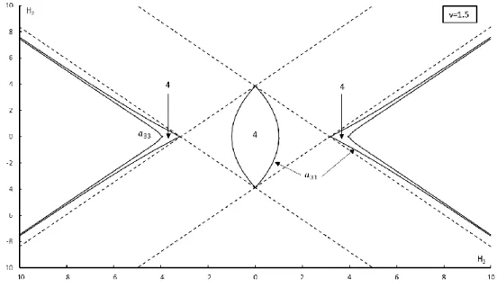
Solving the equations (2.20) and (2.48) in the plane (𝐻3, 𝐻2) represents the equilibria bifurcation for cases (𝑎31= 0, 𝑎32≠ 0 and , 𝑎33≠ 0) and (𝑎31≠ 0 and 𝑎32= 𝑎33= 0), an example for 𝑣 = 1.5 is shown in Figure 3.1. For case (𝑎31≠ 0, 𝑎32≠ 0 and 𝑎33≠ 0) is a more difficult problem because solutions of system (2.11) only correspond to an equilibrium position of the gyrostat when inequalities (2.42) and Δ = 𝑐2_{− 4𝑐 𝑐 ≥ 0 are valid. The regions in the plane (𝐻 , 𝐻 ) in}

30

Figure 3.1 – Bifurcation curves for group of solutions I and III for 𝑣 = 1.5.

Analyzing the Figure 3.1, the curves (2.31) and (2.53) divide the plane (𝐻3, 𝐻2) in three sub-regions. If 𝐻₂2 3⁄

+ 𝐻₃2 3⁄ < (𝑣 + 1)2 3⁄ _{, exits 16 solutions (i.e. equilibrium positions), 8 solutions} for each group of solutions I and III; if (𝑣 + 1)2 3⁄ _{< 𝐻}

2 2 3⁄

+ 𝐻₃2 3⁄ < (4(𝑣 + 1))2 3⁄ , there are 12 solutions, 8 solutions from group of solutions III and 4 solutions of group I; and if 𝐻₂2 3⁄

+ 𝐻₃2 3⁄ > (4(𝑣 + 1))2 3⁄ , there are 8 solutions, 4 solutions from each group of solutions I and III. This result is like the ones found in [8].

As mentioned in [8], inequalities (2.42) needs a closer look since they can be valid either for both signs before the square root or only for one sign, which means the existence of equilibrium positions corresponding to both roots of (2.32) or only one root (𝑥2,1 or 𝑥2,2). The analysis of the regions of validity of inequalities (2.42) for each root of (2.32) at 𝑣 = 1.5, considering that 𝑣 > 0, are presented in Figures 3.3 and Figure 3.4. The dashed lines represent when the discriminant (Δ) (2.34) is equal to zero, which is reflected in more detail in Figure 3.2.

Figure 3.3 – Regions of validity of the conditions 𝑎312 ≥ 0 and 𝑎332 ≥ 0 for the positive root of (2.32) at

𝑣 = 1.5.

Figure 3.4 – Regions of validity of the conditions 𝑎312 ≥ 0 and 𝑎332 ≥ 0 for the negative root of (2.32) at

32

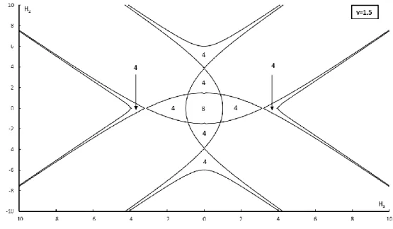
For each case presented in Figures 3.3 and 3.4, the full lines represent when expressions (2.42) are equal to zero. The areas delimited by full lines are regions where the conditions (2.42) are valid for each root of equation (2.32). In each of these regions, there are four solutions of Group II; and beyond their boundaries, there are no solutions, since one or both conditions (2.42) are invalid. Combining results in Figure 3.3 and 3.4, the study of equilibria bifurcation of Group II is achieved in Figure 3.5.

Figure 3.5 – Bifurcation curves for solutions of Group II at 𝑣 = 1.5.

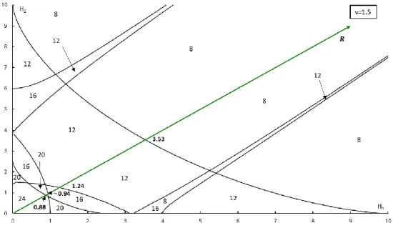
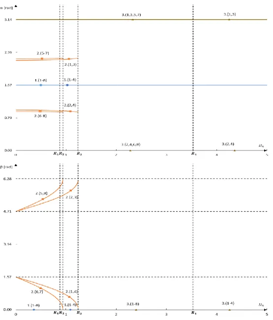
The complete equilibria bifurcation study of the gyrostat at 𝑣 = 1.5, combining the study of bifurcation of solutions of Group I, II and III are presented in Figure 3.6. Notice that the plane (𝐻3, 𝐻2) are portioned into sub-regions, in each of them there are a certain fixed number of equilibrium positions and the curves are symmetric in relation to the origin of the coordinated axes, as mentioned in [14] and [20] by Santos. To help visualize the different conditions of each group I, II and III presented in Figure 3.6, a color notation is used (see table 3.1).