Igor Santos Peretta Evolution of diﬀerential models for concrete systems through Genetic Programming

(1)

UNIVERSIDADE FEDERAL DE UBERLÂNDIA PÓS-GRADUAÇÃO FEELT

Faculdade de Engenharia Elétrica Laboratório de Inteligência Computacional

BRAZIL

UNIVERSITÉ DE STRASBOURG ÉCOLE DOCTORALE 269

Mathématiques, Sciences de l’Information et de l’Ingénieur Laboratoire ICUBE

FRANCE

Joint PhD Thesis

Igor Santos Peretta

Evolution of differential models

for concrete systems through

Genetic Programming

(2)

(3)

UNIVERSIDADE FEDERAL DE UBERLÂNDIA PÓS-GRADUAÇÃO FEELT

Faculdade de Engenharia Elétrica Laboratório de Inteligência Computacional UNIVERSITÉ DE STRASBOURG

ÉCOLE DOCTORALE 269

Mathématiques, Sciences de l’Information et de l’Ingénieur Laboratoire ICUBE

TESE EM COTUTELA

_⋄

THÈSE EN CO-TUTELLE

apresentada por_⋄ présentée par :

Igor Santos Peretta

defesa em _⋄ soutenue le : 21/09/2015

para obtenção do título de : Doutor em Ciências

Área de concentração : Processamento da Informação, Inteligência Artiﬁcial pour obtenir le grade de : Docteur de l’Université de Strasbourg

Discipline/ Spécialité : Informatique

Evolution of differential models for concrete

systems through Genetic Programming

⋄

Evolução de modelos diferenciais para sistemas

concretos por Programação Genética

⋄

Évolution de modèles différentiels de systèmes

concrets par Programmation Génétique

TESE orientada por Prof. Dr. Keiji Yamanaka UFU

⋄ THÈSE dirigée par : Prof. Dr. Pierre Collet, UNISTRA

REVISORES Prof. Dr. Domingos Alves Rade, ITA

⋄ RAPPORTEURS : Prof. Dr. Gilberto Arantes Carrijo, UFU OUTROS MEMBROS DA BANCA Dr. Frederico Gadelha Guimarães, UMFG ⋄ AUTRES MEMBRES DU JURY : Dr. Welsey Pacheco Calixto, IFG

(4)

(5)

Abstract

A system is defined by its entities and their interrelations in an environment which is determined by an arbitrary boundary. Complex systems exhibit emer-gent behaviour without a central controller. Concrete systems designate the ones observable in reality. A model allows us to understand, to control and to predict behaviour of the system. A differential model from a system could be understood as some sort of underlying physical law depicted by either one or a set of differential equations. This work aims to investigate and implement methods to perform computer-automated system modelling. This thesis could be divided into three main stages: (1) developments of a computer-automated numerical solver for linear differential equations, partial or ordinary, based on the matrix formulation for an own customization of the Ritz-Galerkin method; (2) proposition of a fitness evaluation scheme which benefits from the devel-oped numerical solver to guide evolution of differential models for concrete complex systems; (3) preliminary implementations of a genetic programming application to perform computer-automated system modelling. In the first stage, it is shown how the proposed solver uses Jacobi orthogonal polynomials as a complete basis for the Galerkin method and how the solver deals with auxiliary conditions of several types. Polynomial approximate solutions are achieved for several types of linear partial differential equations, including hy-perbolic, parabolic and elliptic problems. In the second stage, the proposed fitness evaluation scheme is developed to exploit some characteristics from the proposed solver and to perform piecewise polynomial approximations in or-der to evaluate differential individuals from a given evolutionary algorithm population. Finally, a preliminary implementation of a genetic programming application is presented and some issues are discussed to enable a better un-derstanding of computer-automated system modelling. Indications for some promising subjects for future continuation researches are also addressed here, as how to expand this work to some classes of non-linear partial differential equations.

(6)

Resumo

Um sistema é definido por suas entidades e respectivas interrelações em um ambiente que é determinado por uma fronteira arbitrária. Sistemas complexos exibem comportamento sem um controlador central. Sistemas concretos é como são designados aqueles que são observáveis nesta realidade. Um modelo permite com que possamos compreender, controlar e predizer o comporta-mento de um sistema. Um modelo diferencial de um sistema pode ser com-preendido como sendo uma lei física subjacente descrita por uma ou mais equações diferenciais. O objetivo desse trabalho é investigar e implementar métodos para possibilitar modelamento de sistemas automatizado por com-putador. Esta tese é dividida em três etapas principais: (1) o desenvolvimento de um solucionador automatizado para equações diferenciais lineares, parci-ais ou ordinárias, baseado na formulação de matriz de uma customização do método de Ritz-Galerkin; (2) a proposição de um esquema de avaliação de aptidão que se beneficie do solucionador numérico desenvolvido para guiar a evolução de modelos diferenciais para sistemas complexos concretos; (3) inves-tigações preliminares de uma aplicação de programação genética para atuar em modelamento de sistemas automatizado por computador. Na primeira etapa, é demonstrado como o solucionador proposto utiza polinômios ortogonais de Jacobi como uma base completa para o método de Galerkin e como o solu-cionador trata condições auxiliares de diversos tipos. Soluções polinomiais aproximadas são obtidas para diversos tipos de equações diferenciais parciais lineares, incluindo problemas hiperbólicos, parabólicos e elípticos. Na segunda etapa, o esquema proposto para avaliação de aptidão é desenvolvido para ex-plorar algumas características do solucionador proposto e para obter aproxi-mações polinomiais por partes a fim de avaliar indivíduos diferenciais de uma população de dado algoritmo evolucionário. Finalmente, uma implementação preliminar de uma aplicação de programação genética é apresentada e algu-mas questões são discutidas para uma melhor compreensão de modelamento de sistemas automatizado por computador. Indicações de assuntos promissores para continuação de futuras pesquisas também são abordadas, bem como a expansão deste trabalho para algumas classes de equações diferenciais parciais não-lineares.

Keywords: Modelamento de Sistemas Automatizado por Computador; Modelos Diferenciais; Equações Diferenciais Ordinárias Lineares; Equações Diferenciais Parciais Lineares; Avaliação de Aptidão; Programação Genética.

(7)

Résumé

Un système est défini par les entités et leurs interrelations dans un environ-nement qui est déterminé par une limite arbitraire. Les systèmes complexes présentent un comportement émergent sans un contrôleur central. Les sys-tèmes concrets désignent ceux qui sont observables dans la réalité. Un modèle nous permet de comprendre, de contrôler et de prédire le comportement du système. Un modèle différentiel à partir d’un système pourrait être compris comme une sorte de loi physique sous-jacent représenté par l’un ou d’un en-semble d’équations différentielles. Ce travail vise à étudier et mettre en œu-vre des méthodes pour effectuer la modélisation des systèmes automatisée par l’ordinateur. Cette thèse pourrait être divisée en trois étapes principales, ainsi: (1) le développement d’un solveur numérique automatisé par l’ordinateur pour les équations différentielles linéaires, partielles ou ordinaires, sur la base de la formulation de matrice pour une personnalisation propre de la méthode Ritz-Galerkin; (2) la proposition d’un schème de score d’adaptation qui bénéficie du solveur numérique développé pour guider l’évolution des modèles différentiels pour les systèmes complexes concrets; (3) une implémentation préliminaire d’une application de programmation génétique pour effectuer la modélisation des systèmes automatisée par l’ordinateur. Dans la première étape, il est mon-tré comment le solveur proposé utilise les polynômes de Jacobi orthogonaux comme base complète pour la méthode de Galerkin et comment le solveur traite des conditions auxiliaires de plusieurs types. Solutions à approximations poly-nomiales sont ensuite réalisés pour plusieurs types des équations différentielles partielles linéaires, y compris les problèmes hyperboliques, paraboliques et el-liptiques. Dans la deuxième étape, le schème de score d’adaptation proposé est conçu pour exploiter certaines caractéristiques du solveur proposé et d’effectuer l’approximation polynômiale par morceaux afin d’évaluer les individus différen-tiels à partir d’une population fournie par l’algorithme évolutionnaire. Enfin, une mise en œuvre préliminaire d’une application GP est présentée et certaines questions sont discutées afin de permettre une meilleure compréhension de la modélisation des systèmes automatisée par l’ordinateur. Indications pour certains sujets prometteurs pour la continuation de futures recherches sont également abordées dans ce travail, y compris la façon d’étendre ce travail à certaines classes d’équations différentielles partielles non-linéaires.

(8)

(9)

Agradecimentos

O processo intenso de realizar uma pesquisa e a posterior redação de uma tese não é um processo individual, mas sim conta com um grande número de pes-soas ligadas direta ou indiretamente. Nessas páginas, gostaria de agradecer a todos aqueles com que me relacionei na minha vida de doutorando no Brasil e os quais, próximos ou distantes, contribuiram para a ﬁnalização dos meus tra-balhos de pesquisa. Infelizmente, esta lista não é conclusiva e não foi possível incluir a todos. Assim, gostaria de exprimir meus agradecimentos ...

À minha esposa Anabela, pela cumplicidade e paciência, e à minha ﬁlha Isis, pela sua subjetiva compreensão, e à ambas pelo amor, apoio em momentos tão difíceis e por estarem sempre ao meu lado me acompanhando em todos os destinos necessários para a conclusão deste trabalho. À minha família, em especial meu pai Vitor, minha mãe Miriam, meus irmãos Érico e Éden, sempre referências em tempos de desorientação, pelo amor, suporte e incentivo incondicionais. À Priscilla, por ajudar a catalizar reﬂexões de doutorado, e à Jussara, pelas conversas sobre rumos de vida. Ao meu sobrinho Iuri, por ter chegado a tempo.

Ao Professor Keiji Yamanaka, meu orientador no Brasil, pela conﬁança em mim depositada, pela presteza em vir ao auxílio, pelas conversas e divisão de angústias, além da grande oportunidade de trabalharmos mais uma vez juntos. Aos Professores Domingos Alves Rade e Gilberto Arantes Carrijo, pela presteza e pontualidade apresentadas para a árdua tarefa de serem pareceristas preliminares desta tese. Ao Professor José Roberto Camacho, pela contagiante paixão, pelo incentivo e pelas muitas discussões. Aos Professores Frederico Guadelha Guimarães e Wesley Pacheco Calixto, pelo entusiasmo e pelo inter-esse demonstrado neste trabalho. A todos inter-esses, obrigado pelas considerações discutidas em tempos de qualiﬁcação e também por aceitarem o convite para participar da banca de defesa.

Ao grande Júlio Cesar Ferreira, por compartilhar angústias, receios e con-hecimentos, além de ter sido um porto seguro em tempos de aventuras além-mar.

(10)

Aos companheiros de laboratório: Juliana Malagoli, Cássio Xavier Rocha, Walter Ragnev, Adelício Maximiano Sobrinho, pelas amizades e pela divisão de saberes e angústias. Aos amigos de UFU, Fábio Henrique “Corleone” Oliveira e Daniel Stefany, pelo suporte e incentivo nas horas mais inusitadas.

Aos técnicos da CAPES: Valdete Lopes e Mailson Gomes de Sousa, que com presteza me auxiliaram no processo de ida e volta da França.

Ao programa de pós-graduação da Faculdade de Engenharia Elétrica, em especial à Cinara Mattos, pela simpatia, presteza e solidariedade mesmo nas situações mais difíceis. Aos professores Alexandre Cardoso, Edgard Afonso Lamounier Júnior, Darizon Alves de Andrade, cada qual ao seu tempo, pela atenção necessária a ﬁm de realizar esta pesquisa.

Aos professores Alfredo Júlio Fernandes Neto e Elmiro Santos Resende, cada qual em seu tempo de Reitor da Universidade Federal de Uberlândia, pela atenção necessária para a realização deste doutorado em cotutela.

Ao casal Fábio Leite e Silvia Maria Cintra da Silva e à Carmen Reis, pela grande amizade e pelo apoio familiar tão importante nesses tempos de doutorado.

Aos amigos da DGA na UNICAMP, pelo importante apoio no começo de minha jornada: Maria Estela Gomes, Pedro Emiliano Paro, Edna Coloma, Lúcia Mansur, Elsa Bifon, Soninha e Pedro Henrique Oliveira.

Aos amigos de Campinas: Carlos Augusto Fernandes Dagnone, Marco Antônio Zanon Prince Rodrigues, Bruno Mascia Daltrini, Daniel Granado, Alexandre Martins, Sérgio Pegado, Alexandre Loregian, João Marcos Dadico e Rodrigo Lício Ortolan. pela longa amizade e pela caminhada que trilhamos juntos. Estaremos sempre próximos, mesmo que distantes.

(11)

Remerciements

Le processus intensif de poursuivre la recherche et la rédaction d’une thèse n’est pas un processus individuel, mais on peut impliquer des nombreuses person-nes, directement ou indirectement. Dans ces pages, je tiens à remercier toutes celles et ceux que j’ai rencontré durant ma vie de doctorant en France et qui, de près ou de loin, ont contribué à la réussite de mes travaux de recherche. Mal-heureusement, cette liste n’est pas exhaustive et ce n’est pas possible d’inclure tout le monde. C’est pourquoi je voudrais exprimer mes remerciements ...

Au Professeur Pierre COLLET, mon directeur de thèse en France, pour avoir établi une conﬁance en moi, les discussions sur le sujet de cette recherche et les indications aﬁn de consulter divers experts. Aussi, pour le soutien continu au niveau académique et personnel. C’était une opportunité exceptionnelle de pouvoir travailler avec vous.

Au Professeur Paul BOURGINE, pour l’intérêt, le soutien, l’attention, mais surtout pour l’accueil et la générosité de partager des enseignements et des idées essentielles à cette recherche.

Au Professeur Jan DUSEK, à bien des discussions sur le sujet de cette thèse, et à Professeure Myriam MAUMY-BERTRAN, tous les deux pour faire partie du comité de suivi de thèse.

Au Professeur Thomas NOËL, en acceptant d’être le rapporteur français de cette thèse.

A mes compagnons « d’armes »: Andrés TROYA-GALVIS, Bruno BE-LARTE, Carlos CATANIA, Clément CHARNAY, Karim EL SOUFI, Manuela YAPOMO, Joseph PALLAMIDESSI, Wei YAN, Chowdhury FARHAN AHMED et tous les stagiaires qui ont été proche de moi pendant cette année en France. Merci pour l’accueil chaleureux, pour les enseignements et pour l’amitié qui restera, bien j’espère longtemps.

À Julie THOMPSON et au Olivier POCH, pour l’accueil sympathique et l’amitié manifestée.

A l’équipe BFO, les MCF Nicholas LACHICHE, Cecilia ZANNI-MERK, Stella MARC-ZWECKER, Pierre PARREND, François de Bertrand DE BEU-VRON et Agnès BRAUD. Aussi, à les Professeurs Pierre GANÇARSKI et Christian MICHEL. C’était un honneur de travailler avec vous.

Aux anciens doctorants Frédéric KRÜGER et OGIER MAITRE, et l’ancienne post-doc Lidia YAMAMOTO, pour le guidage, même que nous ne nous ren-contrâmes pas en personne.

(12)

À Laboratoire ICUBE, je voudrais spécialement remercieer Mme Christelle CHARLES, Mme Anne-Sophie PIMMEL, Mme Anne MULLER, Mme Fabi-enne VIDAL et le directeur Professeur Michel DE MATHELIN, pour l’accueil sympathique et l’attention particulière.

À École Doctorale MSII, en particulier à Mme Nathalie BOSSE, pour le soutien et l’attention toujours manifestés.

À UFR Mathématique-Informatique, je tiens en particulier à remercier Mme Marie Claire HANTSCH, pour l’accueil sympathique et chaleureux.

À Université de Strasbourg, je remercie Mme Isabelle LAPIERRE, pour le soutien et l’attention particulière.

Aux Professeurs Yves REMOND, directeur de l’École Doctorale, et Alain BERETZ, le président de l’Université de Strasbourg, pour l’attention néces-saire à la réalisation de ce doctorat en co-tutelle.

Aux amis en France: Laurent, Anna Lucas et famille KONDRATUK; Caro-line et famille VIRIOT-GOELDEL; Ignacio, Sara et famille GOMEZ MIGUEL; Franck, Karine et famille HAGGIAG GLASSER, pour tous les moments passés ensemble et l’amitié éternelle.

Enﬁn, à Mme Marie Louise KOESSLER, en raison des cours de français donnés et des révisions éventuelles, mes très chaleureux remerciements.

(13)

Acknowledgements

This research was funded by the following Brazilian agencies:

• Conselho Nacional de Desenvolvimento Cientíﬁco e Tecnológico (CNPq), full PhD scholarship category GD, while in Brazil;

(14)

A journey of a thousand miles starts beneath one’s feet.

(15)

List of Figures

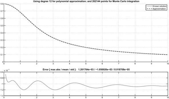
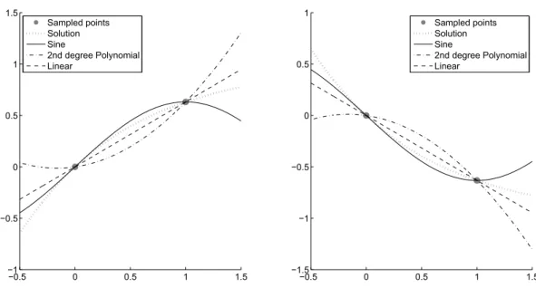
1.1 A situational example where diﬀerent methods for conventional re-gression (linear, piece-wise 5th degree polynomial, spline) fail to ﬁnd a known solution from a not so well behaved randomly sam-pled points. . . 5 1.2 Hypothetical situation, two points sampled from each concrete

sys-tem. (left) Known describing function is f(x) = 1₋e−x_{; (right)} Known describing function is g(x) = e−x₋₁_{. . . .} ₆ 3.1 Monte Carlo integration performance on f(x, y) = exp(₋x) cos(y)

deﬁned in _{0_≤x_≤1; 0_≤y_≤ π₂_} (100 runs). . . 26

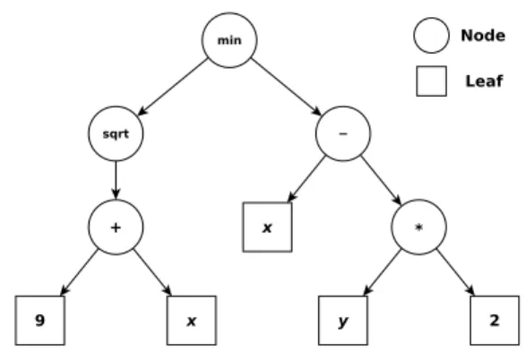
3.2 EA ﬂowchart: each loop iteration is a generation; adapted from [75] 29 3.3 Example of an abstract syntax tree for the computation “min(√9 +x, x₋

2y)”, or, in RPN, (min (sqrt (+ 9 x)) (- x (* 2 y))) . . . 30

3.4 Summary of this simple run (see Table 3.2); darker elements were randomly generated; dashed arrows indicates cut points to mix genes in related crossovers; adapted from [13]. . . 31

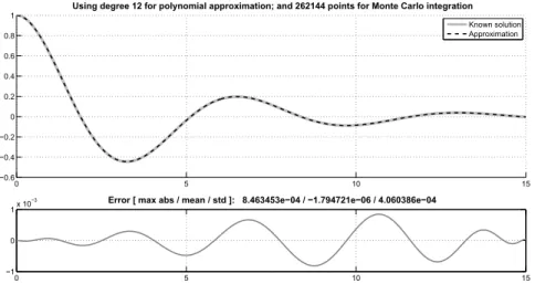
4.1 Solution to an under-damped oscillator problem, polynomial ap-proximation of degree 12. . . 42 4.2 Solution to a Poisson equation for electrostatic subject to a static

spherically symmetric Gaussian charge density, polynomial approx-imation of degree 12. . . 45 4.3 Approximation by the proposed method to the ODE that generated

Figure 1.2, left plot; same diﬀerential as in Figure 4.4, diﬀerent boundary conditions. Solution y(x) = 1₋exp(₋x) approximated

to: yˆ(x) = 5.15 10−3_x5

−3.86 10−2_x4_{+ 1}_._{65 10}−1_x3

−5.00 10−1_x2₊

1.00x. . . 46

4.4 Approximation by the proposed method to the ODE that generated Figure 1.2, right plot; same diﬀerential as in Figure 4.3, diﬀerent boundary conditions. Solution y(x) = exp(₋x)₋1 approximated

to: yˆ(x) =₋5.15 10−3_x5₊₃_._{86 10}−2_x4₋₁_._{65 10}−1_x3₊₅_._{00 10}−1_x2₋

1.00x. . . 46

5.1 Solution to a dynamic one-dimensional wave problem; approximate solution adopts a degree 8 bivariate polynomial. . . 58 5.2 Solution to a homogeneous heat conduction equation with

insu-lated boundary; approximate solution adopts a degree 11 bivariate polynomial. . . 60

(19)

List of Figures

5.3 Solution to a steady-state temperature in a thin plate (Laplace equation); approximate solution adopts a degree 9 bivariate poly-nomial. . . 63

6.1 Preparation steps for the proposed fitness evaluation method; dashed border nodes can benefit from parallelism. . . 67 6.2 Flowchart for the proposed fitness evaluation method; dashed

bor-der nodes can beneﬁt from parallelism. . . 68 6.3 Overlap of solution plot and piecewise approximations for the

under-damped oscillator problem; overall ﬁtness evaluated as4 10−4_{. (top)}

All 13 piecewise domains and approximations. (low left) Approxi-mation over the 2nd considered domain. (low center) Approxima-tion over the 7th considered domain. (low right) ApproximaApproxima-tion over the 11th considered domain. . . 72 6.4 Overlap of solution plot and piecewise approximations for the

Pois-son electrostatics problem, overall ﬁtness evaluated as 7.44 10−6_.

(top) All 13 piecewise domains and approximations. (low left) Ap-proximation over the 2nd considered domain. (low center) Approxi-mation over the 7th considered domain. (low right) ApproxiApproxi-mation over the 11th considered domain. . . 75

7.1 An example of model candidate representation, a vector of AAST’s. This example represents the LPDE[5 cos (πx)]_· ∂2

∂y2u(x, y) + [−2.5]· ∂

∂x ∂

∂yu(x, y)+ [

exp( −y2

)

+x] · ∂

∂yu(x, y)+[1]·u(x, y) = sin (πx) cos (πy) and each coefficient (an AAST) is supposed to be built at random for a deterministic vector which length and element meanings are based on user’s definition of order 2 for differentials regarding a

system whose measurements covers 2 independent variables (x, y). . 77

7.2 Types of binary operators. Shaded elements represent random cho-sen points for operations. (left) Type-I recombination. (center) Type-II recombination. (right) Type-III recombination. . . 78 7.3 Types of unary operations. Shaded elements represent random

cho-sen points for operations. (left) Classic-like mutation. (center) Mu-tation by pruning. (right) MuMu-tation by permuMu-tation. . . 79

8.1 Plot for the best individual ﬁtness through generations. Note that, in this very example, the convergence to the solution is already stabilized by the 25th generation. . . 86 8.2 Overlap of solution plot and piecewise approximations for the

(20)

List of Figures

8.3 White Gaussian noise (WGN) added to signal. (a) Half-period sine signal, no noise added. (b) WGN 100dB added to signal; error distribution with mean e¯ = 4.25 10−7 _{and standard}

devia-tion s = 4.25 10−7_{. (c) WGN 50dB;} _¯_e _{= 8}_._{08 10}−5_, _s _{= 2}_._{24 10}−3_.

(d) WGN 40dB; e¯ = 1.58 10−3_, _s _{= 7}_._{33 10}−3_{. (e) WGN 25dB;}

¯

e = ₋9.21 10−4_, _s _{= 3}_._{81 10}−2_{. (f) WGN 10dB;} _e_¯ ₌ ₋₃_._{34 10}−2_,

s= 2.05 10−1_{. . . 88}

B.1 Example on CUDA C. (left) Standard C Code; (right) Parallel C Code; adapted from website http://www.nvidia.com . . . 95

C.1 Example of EASEA syntax for speciﬁcation of a Genome Evaluator 97

(21)

List of Tables

3.1 Monte Carlo integration applied to f(x, y) = exp(₋x) cos(y)

de-ﬁned in _{0_≤x_≤1; 0 _≤y _≤ π

2 } (100 runs). . . 25

3.2 Preparation step for function approximation; adapted from [13]. . . 30 3.3 Summary of this simple run (see Figure 3.4); note that there is a

match (found solution) in generation 1; adapted from [13] . . . 31

5.1 Types of PDE, adapted from [81]. . . 49 5.2 Examples of integer partition of numbers 0 upto 3 with 2 parts

maximum (Algorithm 2) and 3rd _{degree polynomials or} ₃rd _order derivatives with2variables (Algorithm 3); this should be called the

powers matrix. . . 52

6.1 Example of a data ﬁle with3independent variables and1dependent

variable (quantity of interest representing a scalar ﬁeld). . . 69 6.2 TGE coeﬃcients retrieved for the under-damped oscillator example,

each set related to one of 13 groups of points. . . 73 6.3 TGE coeﬃcients retrieved for the Poisson electrostatics example,

each set related to one of 13 groups of points. . . 74

(22)

List of Algorithms

1 Practical condition test; test if a coeﬃcient matrix is well-conditioned or not. . . 21 2 Integer Partition; enlisted inoutare all unique possibilities of

v summands for the integern, regardless order; adapted from [82] 50

3 Powers Matrix, enlisted inpowsare the multivariate (v

vari-ables) polynomialn-degrees or diﬀerentialn-orders. . . 51

(23)

List of Acronyms

CASM Computer-Automated System Modelling

EA Evolutionary Algorithm

EC Evolutionary Computation

FEM Finite Element Method

GP Genetic Programming

GSE Galerkin System of Equations

LDE Linear Diﬀerential Equation

LODE Linear Ordinary Diﬀerential Equation

LPDE Linear Partial Diﬀerential Equation

ODE Ordinary Diﬀerential Equation

PDE Partial Diﬀerential Equation

SNR Signal-to-Noise Ratio

TGE Truncate Galerkin Expansion

(24)

(25)

Part I

(26)

Chapter 1 Introduction

1.1 Overview

A system is defined by its interrelated parts, also known as entities, surrounded by an environment which is determined by an arbitrary boundary. More in-sights on the definition of a system could be achieved by accessing the work of [1]. This present work considers a system of interest as being concrete (in contrast to abstract) and possibly closed, even when it could be classified as open. The former classification means that the system can exist in this reality. The latter means that every entity has some relations with others, i.e., if an entity is part of a system, that means it can affect and be affected by others, directly or indirectly, and is also responsible in some degree for the overall behaviour that the system presents.

A concrete system could be object of a simplified representation, known as a model, in order to be understood, to explain its behaviour with respect to its entities and to enable simulations and predictions of its behaviour accord-ing to an arbitrary initial state. In reality, it is usual to not totally represent a concrete system due to the great number of constituent entities involved together with a large set of complex interrelations. Normally, to build such representation (known as a model) is to optimize the compromise between sim-plification and accuracy. This work is interested about in silico models which refers to “simulations using mathematical models in computers, thus relying on silicon chips” [2]. The process of building such model to a system, approxi-mately and adequately, needs to rely on its most relevant entities (independent variables) that have influence on the overall system behaviour (represented by one or more dependent variables). This process is widely known as System Modelling. Note that, as stated by [1], the number of significant entities and relations could change depending on the arbitrary determination of a bound-ary.

A representative model could be understood as some sort of underlying physical law [3, 4], or even a descriptor which could fulﬁl the variational prin-ciple of least action1 _{[5, 6]. As stated by [7], “many physical processes in nature} [...] are described by equations that involve physical quantities together with

1

(27)

1.2. Motivation

their spatial and temporal rates of change”. Actually, observations of natu-ral phenomena were responsible to the early developments of the infinitesimal calculus discipline [8]. In other words, due to its properties of establishing connections and interactions between independent and dependent entities (e.g. physical, geometrical, relational), models to systems are expected to be one or a set of differential equations [9]. An ordinary differential equation (ODE), if only one entity is considered responsible for the behaviour of a system, or more commonly a partial differential equation (PDE) can describe how some observable quantities change with respect to others, tracking those changes throughout infinitesimal intervals.

Presenting as a simple example, the vertical trajectory of a cannonball when shot in an ideal scenario could be modelled by the ODE g+ d2

dt2y(t) = 0.

This equation presents the relation between the unknown function y(t) —

the instantaneous height of the cannonball relative to an inertial frame of reference with respect to a relative measure of time t — and the acceleration

of gravity g. Initial state conditions such as d dty(t)

t=0 = V0 and y(0) = H0

eﬀectively lead to the following well known solution: y(t) = H0+V0t−g t

2

2 . This

solution to that differential model describes with ideal precision the cannonball vertical trajectory. If this system can be kept closed to outer entities (e.g., air friction, strong winds), the mentioned differential model would still be the same, no matter the fact that different initial states could lead to different vertical trajectory solutions.

From the point of view of engineering, this work is interested in concrete systems whose entities enable some kind of quantitative measurements for related quantities2_{. If those measurements are taken from the main entities} responsible for the behaviour of the system, then it is fair to suppose that an accurate enough model could be built.

Nowadays, the necessity for models is increasing, once science is dealing with concrete systems that could display a huge dataset of observations (Big Data researches) or even present chaotic behaviour (dynamic or complex sys-tems). This work goes further into this idea and investigates how system modelling could be automated. This thesis is part of a research aimed to miti-gate diﬃculties and propose methods to enable a computer-automated system modelling (CASM) tool to construct models from observed data.

1.2 Motivation

When deﬁning a system of interest, researches intent to describe a great vari-ety of phenomena, from Physics and Chemistry to Biology and Social sciences. Systems modelling have applications to problems of engineering, economics, population growth, the propagation of genes, the physiology of nerves, the regulation of heart-beats, chemical reactions, phase transitions, elastic buck-ling, the onset of turbulence, celestial mechanics, electronic circuits [10], ex-tragalactic pulsation of quasars, ﬂuctuations in sunspot activity on our sun,

2

(28)

1. Introduction

changing outdoor temperatures associated with the four seasons, daily temper-ature ﬂuctuations in our bodies, incidence of infectious diseases, measles to the tumultuous trend of stock price [11], among many others examples. Models are essential to correctly understand, to predict and to control their respective systems. An inaccurate model will fail to do so.

The classic approach for system modelling is to apply regressions techniques of some kind on a set of measurements in order to retrieve a mathematical function that could explain that dataset.

Regression techniques involve developing causal relations (functions) of one or more entities (independent variables) to a sensible eﬀect or behaviour (de-pendent variable of interest). Historically, those techniques have being used to system modelling starting from observed data. There are two main approaches to regression: classic (or conventional) regression and symbolic regression.

Conventional regression starts from a particular model form (a mathemat-ical expression with a known structure) and follows by using some metrics to optimize parameters for a pre-specified model structure supposed to best fit the observed data. A clear disadvantage is that, after parametrized by using ill-behaved data, the chosen model could not be useful at all, or even work just within a limited region of the domain, failing in other regions. A specific difficult dataset example is shown in Figure 1.1. There, different conventional regression techniques fail to rediscover a known function from its randomly sampled sparse points. Note that, to achieve the full potential of those tech-niques, data must be well behaved (e.g., equidistant points) and be available in a sufficient amount.

While conventional regression techniques seek to optimize the parameters for a pre-speciﬁed model structure, symbolic regression avoids imposing prior assumptions, and, instead, infers the model from the data.

Symbolic regression, in the other hand, searches for an appropriate model structure rather than imposing some prior assumptions. Genetic Program-ming (GP) is widely used for this purpose [12, 13]. GP is based on Genetic Algorithms (GA) and belongs to a class of Evolutionary Algorithms (EA) in which ideas from the Darwinian evolution and survival of the fittest are roughly translated into algorithms. Therefore, GP is known to evolve a model struc-ture side-by-side with the respective necessary parameters. Also, there is the theoretical guarantee (in infinite time) that GP will converge to an optimum model3_{able to fit the observed data. As an example, if trigonometric functions} are available as building blocks, Genetic Programming is capable of converging to the function

y(x) = 3 sin(π x)cos(16π x)

which is the correct function subjected to the sampling of points at random back in Figure 1.1.

To understand why this work does not simply use symbolic regression, take a close look at Figure 1.2. Both left and right plots show only two sampled points. Lets imagine this hypothetical situation where there are concrete sys-tems, the “left” one and the “right” one, and from both there are only two

3

(29)

1.2. Motivation

0 0.1 0.2 0.3 0.4 0.5 0.6 0.7 0.8 0.9 1

4 3 2 1 0 1 2 3

4 Solution

Sampled points Linear

Piecewise 5th degree polynomial Spline

Figure 1.1: A situational example where diﬀerent methods for conventional regression (linear, piece-wise 5th degree polynomial, spline) fail to ﬁnd a known solution from a not so well behaved randomly sampled points.

measurements available for each one. The known behaviour of those systems are respectively described by

f(x) = 1₋e−x and g(x) =e−x₋1.

The left plot also presents among other inﬁnite possibilities the following func-tions that pass through the same two sampled points:

(sine) fs(x) = 0.6321 sin(π₂x) (polynomial) fp(x) = 0.4773x2+ 0.1548x (linear) fl(x) = 0.6321x.

The right plot also presents the functions:

(sine) gs(x) =−0.6321 sin(π₂x) (polynomial) gp(x) = −0.4773x2−0.1548x (linear) gl(x) =−0.6321x.

Note that they are one the mirror image of the other (related to the horizontal axis through f(x) = g(x) = 0), but lets move this information aside for a

moment.

Actually, both plots refer to solutions for the same ODE:

d2

dx2y(x) +

d

dxy(x) = 0

with diﬀerent initial values, for the plot on the left:

d dxy(x)

x=0

(30)

1. Introduction

−0.5 0 0.5 1 1.5

−1

−0.5 0 0.5 1 1.5

Sampled points Solution Sine

2nd degree Polynomial Linear

−0.5 0 0.5 1 1.5

−1.5

−1

−0.5 0 0.5 1

Sampled points Solution Sine

2nd degree Polynomial Linear

Figure 1.2: Hypothetical situation, two points sampled from each concrete system. (left) Known describing function is f(x) = 1₋e−x_{; (right) Known} describing function is g(x) =e−x₋₁_.

and, for the plot on the right:

d dxy(x)

x=0

=₋1 and y(0) = 0.

Assuming the differential model for those systems is known, the solution of this ODE not only supplies a reliableinterpolation function between those two points, but a reliable extrapolation function as well. The process of solving a differential model could benefit from measurements to infer initial states or boundaries and the solution would be valid as long as neither involved entities (tracked by independent variables) vanish nor others appear.

This hypothetical situation shows the possibility of the same model rep-resenting either two separate systems or the same system presented in two diﬀerent states. As could be inferred, awareness of the initial state leads the model to present itself as having a unique solution. A purely symbolic regres-sion approach would have two major diﬃculties when considering this very situation here4_{: (a) all enlisted functions —} _f

s(x), fp(x), fl(x), gs(x), gp(x),

gl(x) — would be considered valid solutions, as the same for any of the inﬁ-nite possible functions that pass exactly through those two points; (b) each situation represented by both left and right systems have a high probability of having a diﬀerent function model and, in this case, no relation between them would be uncovered. In other words, symbolic regressionper se would not have enough information to even start to raise questions about similarities between those two systems. One could state that symbolic regression is directed to

4

(31)

1.3. Thesis Statement

model only one “instantiation” of the system (a single possible initial state or adopted boundary) at a time.

Another argument, as known to those dealing with physics and calculus of variations, the action functional (a path integration) is an attribute of a system related to a path, i.e., a trajectory that a system presents between two boundary points in space-time. The principle of least action (also known as the principle of stationary action) states that such system will always present a path over which this action is stationary (an extreme, usually minimal and unique) [6]. This path of least action (the integrand of the action) is often described by a diﬀerential equation and describes the intrinsic relations of a system, the very type of diﬀerential model this work is aimed to look for.

Following this path, it is pretty straightforward to reach the conclusion that a CASM tool should search for differentials whose solutions could explain the observed data. Also, this tool should not keep the search within the domain of mathematical expressions, as done by classic symbolic regression. The domain of search becomes the space of differential equations. In that way, discussions about a possible unification for both left and right aforementioned systems would be possible. Such approach would be concerned about the model of the system itself, whichever “instantiation” (possible initial states or adopted boundary) it has been presented.

Given the domain of search for a model as the space of possible differ-ential equations and concepts behind the principle of least action, this work starts from the idea that every observable concrete system from which some quantitative measurements could be taken is a valid candidate to construct a model. As stated in [14], “the idea of automating aspects of scientific activity dates back to the roots of computer science” and this research is no different. This work intends to investigate a possible way to enable CASM. Looking for-ward, as that work concluded, “human-machine partnering systems [...] can potentially increase the rate of scientific progress dramatically” [14].

1.3 Thesis Statement

One of the essential objectives of this work is to develop a computer-automated numerical solver for linear partial diﬀerential equations in order to assist a Genetic Programming application to evaluate ﬁtness of model candidates. The provided input for the Genetic Programming application should be a dataset containing measurements taken from observations of the system of interest.

Research questions

Some questions have been guiding this research:

• Given a database which contains measurements from an observable con-crete system, is there a more robust way to verify how ﬁt is a theoretical model to this system, relying on those available data?

(32)

1. Introduction

• Would such CASM tool be able to rediscover known models, propose modiﬁcations to them, or even reveal previously unknown models?

This thesis presents answers to the ﬁrst two questions. The third one is partially answered, though. This is an open work in the sense that it points to several branches of possible research to be carried on.

Objectives

In this section, the general and speciﬁc objectives are presented.

General

Achieve a linear diﬀerential equation numerical solver to support a concrete system modelling tool which uses Genetic Programming to evolve sets of partial diﬀerential equations. A dataset of observations must be available.

Specific

• Develop a computer-automated numerical solver for linear partial differ-ential equations with no restrictions besides linearity. The solver must assist the evolutionary search of the Genetic Programming application by enabling fitness evaluation of individuals constituted by linear partial differential equations.

• Develop a syntax tree representation for a candidate solution and a proper module for ﬁtness evaluation in consonance with the proposed solver.

• Run some case studies where the observations dataset is generated through simulation of a known model; provide those simulated data as inputs to the Genetic Programming application with the intention of evolving the model to the known solution, turning this exercise into an inverse prob-lem resolution.

• Evaluate the impact of adding noise to input data regarding the evolu-tion of a previous known model. This should enable discussions about tolerance for measurements related to the system of interest.

• Identify and propose derived branches for future works.

1.4 Contributions

The present work brings the following contributions:

(33)

1.5. Research tools

of systems of linear equations (e.g. using metrics and procedures as rank, condition, pseudoinverse). The achieved solution is a polynomial approximation of the diﬀerential solution.

• A generic scheme to a computer-automated numerical solver for linear partial differential equations (ordinary ones included) using polynomial approximations for the differential solution. Also, the knowledge to ex-pand this solver to some non-linear differential equations is already gath-ered and it is planned for the near future.

• A dynamic ﬁtness evaluation scheme to be plugged into evolutionary al-gorithms to automatically solve linear diﬀerential equations and evaluate model candidates.

This work had to restrict itself to linear differential equations, though, but those models could present any structure inside the linearity restriction. Besides, the same method is used to both ODEs and PDEs. Indeed, the search for differential models has been tried before. Even so, authors have no knowledge of works which could deal with systems in general but the ones where further specifications on the form of the model is required.

1.5 Research tools

Numerical methods

As stated by [7], one of the “most general and efficient tool for the numerical solution of PDEs is the Finite element method (FEM)”. Some limitations do not allow this work to follow this suggested path, though. FEM[15, 16, 17, 7] starts from solving a differential equation (or a set of) in order to present results over a mesh of points throughout the domain. The type of modelling this work is interest on implies in having the actual results of some system on some points over the domain and trying to recover the differential which could explain the behaviour of the system. This is an inverse problem and FEM could not help but to inspire some solutions here presented.

As could be imagined, the method of searching for differential equations must solve at some point those differentials in order to verify the quality of a model candidate. Moreover, integrals should also be useful. The classical and widely used numerical tools to do the job are: (a) using the technique of separating variables to partial differential equations and applying Runge-Kutta methods to approximate solutions for the achieved ordinary differential equations; and (b) Gauss Quadrature methods to perform numerical integra-tions for arbitrary funcintegra-tions [18, 19], multidimensional cases covered by tensor products or sparse grids [20, 21]. Numerical methods designed to directly solve partial differential equations are seldom explored in the literature, due to the success of the aforementioned methods, and the growing need for multidimen-sional integration (cubature) methods keeps it as an open research topic.

(34)

1. Introduction

operations are necessary, especially when dealing with partial differential equa-tions. Parallelism is also desirable, once the entire process has the potential to be an eager customer of computational power. The possibility of trans-forming it into a Linear Algebra problem, as could be seen when dealing with FEM, is also very tempting. After a long period of experimentations and aim-ing for those purposes, this work has finally adopted the followaim-ing numerical methods: (a) the Ritz-Galerkin method [22], specifically an own customiza-tion of the method, to build a system of equacustomiza-tions from differential equacustomiza-tions (ordinary or partial); (b) Monte Carlo integration [23] to perform multivari-ate integrals; and (c) matrix formulations with relmultivari-ated operations to evalumultivari-ate candidate models.

Evolving models

The GP technique is classified under the Evolutionary Computation (EC) re-search area in which, as suggested by its name, covers different algorithms that draw inspiration from the process of natural evolution [24]. GP is, at the most abstract level, a “systematic, domain-independent method for getting comput-ers to solve problems automatically starting from a high-level statement of what needs to be done” [13]. That is an expected quality for evolving models by GP which is known to to find previous unthoughtful solutions for unsolved problems so far [25]. This feature could only be accessed if GP is allowed to build random individuals from a unconstrained search space.

Implementing CASM through GP have been proven the right choice in the literature, specially when modelling functions from data [26, 4, 27, 28]. For a system of interest with available measurements, this works instead aims to evolve a functional (partial diﬀerential equation) whose solution is a function that could explain the available data. Classic GP symbolic regression needs some adjustments to be able to do so.

Computer programming language

The chosen language for programming is C++. Besides high speed perfor-mances [29], C++ language has been listed on the top 5 programming lan-guages rank [30], has support for several programming paradigms (e.g., im-perative, structured, procedural and object-oriented), has a large active com-munity, could beneﬁt from 300+ open source libraries [31] (including 100+ of

boost set of libraries only) and several others freely distributed (e.g. BLAS

and LAPACK5 _{for linear algebra purposes; MPICH2, CUDA and OpenCL for} parallel/concurrency programming), and allows the programmer to take con-trol of every aspect of programming. In the other hand, C++ is strongly plat-form based (code has to be compiled in whatever operational system and/or hardware the executable is needed to run on) and the programmer has to be aware of every aspect of programming (depending on the aimed application, programmer also needs to know about the hardware involved). Those pros and cons were evaluated before this choice, including the need this project has for high performance computation.

5

(35)

1.6. Outline of the text

1.6 Outline of the text

This thesis is divided into three parts. The first one, Background, covers this introduction in Chapter 1. A non comprehensive list of related works that deal with system modelling through Genetic Programming is presented in Chap-ter 2. Related theory in ChapChap-ter 3 are addressed in order to understand the method proposed here: linear differential equations, Hilbert inner product and basis for function spaces, Ritz-Galerkin method, well-possessedness of a differ-ential problem, Jacobi polynomials, linear mappings and change of variables, Monte Carlo integration and Genetic Programming.

The second part refers to the proposed method itself. It starts by explain-ing how the proposed method could be applied to linear ordinary diﬀerential equations in Chapter 4. The extension of those results when applying the method to linear partial diﬀerential equations is shown in Chapter 5.

(36)

Chapter 2 Related Works

2.1 A brief history of the field

Since decades ago, scientists have been trying to build models from observable data. Once datasets of interest starts to increase and underlying model struc-tures became complicated to infer, scientists start thinking about automating the modelling process.

One of the first works that authors could find, the work of Crutchfield and McNamara [32] in 1987 shows the development of a numerical method based on statistics to reconstruct motion equations from dynamic/chaotic time-series data. In a subsequent work, Crutchfield joined Young [33] to address updates to that approach while introducing a metric of complexity for non-linear dy-namic systems.

Still in the 1980’s, some researchers had developed techniques capable of evolving computer programs, like the works of Cramer, Hicklin and Fu-jiko [34, 35, 36], respectively, as an attempt to inspire “creativity” into com-puter machines. These eﬀorts culminate with the advent of Genetic Program-ming with the works of Koza [37, 12] to enable science in the 1990’s to start experiencing computer-automated symbolic regression in the form of mathe-matical expressions constructed from data. In general, all family of Evolution-ary Algorithms [38, 39, 40, 24] could be easily related with system modelling, but GP brought a lot of facilities and powerful tools into the subject [13].

Nevertheless, the work of Schmidt and Lipson [4] published in 2009 is often seen by the scientiﬁc community as a great landmark for computer-automated system modelling due to the broad impact it had on the media at the time it was published (e.g., articles in [41, 42, 43]). Even considering that some relevant issues were raised by Hillar [44], Schmidt and Lipson provided observations from basic lab experiments to a computer and this computer was able, using GP-like techniques, to evolve some underlying physical laws in the form of mathematical expressions with respect to the phenomena addressed in the experiments, using 40 minutes to a few hours to do so, depending on the problem.

(37)

2.2. Early papers

pointed out that “computers with intelligence can design and run experiments, but learning from the results to generate subsequent experiments requires even more intelligence”. This work has the perspective that computer-automated system modelling must be aimed to help scientists to understand, predict and control their object of study.

Therefore, this section is aimed to cover works that are relate to this thesis within the subject of computer-automated system modelling from observable data. Only works that also make use of GP or some other EA are addressed here. Note that the following list is not intent to be comprehensive, but should reﬂect the state of art in this ﬁeld. The list is sorted from the early years to nowadays. When two or more works are from the same year, sort criteria turns to be lexicographic.

2.2 Early papers

before 2000

Gray et al. [26] uses GP to identify numerical parameters within parts of the non-linear differential equations that describes a dynamic system, starting from measured input-output response data. The proposed method is applied to model the fluid flow through pipes in a coupled water tank system.

2000 up to 2004

Cao et al.[45] describes an approach to the evolutionary modelling problem of ordinary differential equations including systems of ordinary differential equa-tions and higher-order differential equaequa-tions. They propose some hybrid evo-lutionary modelling algorithms (genetic algorithm embed in genetic program-ming) to implement the automatic modelling of one and multi-dimensional dynamic systems respectively. GP is employed to discover and optimize the structure of a model, while GA is employed to optimize its parameters.

Kumon et al. [46] present an evolutionary system identiﬁcation method based on genetic algorithms for mechatronics systems which include various non-linearities. The proposed method can determine the structure of linear and non-linear elements of the system simultaneously, enabling combinatorial optimization of those variables.

Chen and Ely [47] compare the use of artificial neural networks (ANN), ge-netic programming, and mechanistic modelling of complex biological processes. They found these techniques to be effective means of simulation. They used Monte Carlo simulation to generate sufficient volumes of datasets. ANN and GP models provided predictions without prior knowledge of the underlying phenomenological physical properties of the system.

Banks [48] presents a prior approach to model Lyapunov functions. He has implemented a GP, in Mathematica_⃝R, which searches for a Lyapunov function

(38)

2. Related Works

Leung and Varadan [49] propose a variant to GP in order to demonstrate its ability to design complex systems that attempts to reconstruct the functional form of a non-linear dynamical system from its noisy time series measurements. They did diﬀerent tests on chaotic systems and real-life radar sea scattered signals. Then they apply GP to the reverse problem of constructing optimal systems for generating speciﬁc sequences called spreading codes in CDMA communications. Based on computer simulations, they have shown improved performance of the GP-generated maps.

Hinchliﬀe and Willis [50] uses multi-objective GP to evolve dynamic process models. He uses GP ability to automatically discover the appropriate time history of model terms required to build an accurate model.

Xiong and Wang [51] propose both a new GP representation and algorithm that can be applied to both continuous and discontinuous functions regression applied to complex systems modelling. Their approach is able to identify both structure and discontinuity points of functions.

2005 up to 2009

Beligiannis et al. [52] adopts a GP-based technique to model the non-linear system identification problem of complex biomedical data. Simulation results show that the proposed algorithm identifies the true model and the true values of the unknown parameters for each different model structure, assisting the GP technique to converge more quickly to the (near) optimal model structure.

Bongard and Lipson [53], states that uncovering the underlying diﬀerential equations directly from observations poses a challenging task when dealing with complex non-linear dynamics. Aiming to symbolically model complex networked systems, they introduce a method that can automatically generate symbolic equations for a non-linear coupled dynamical system directly from time series data. They state that their method is applicable to any system that can be described using sets of ordinary non-linear diﬀerential equations and have an observable time series of all independent variables.

Iba [54] presents an evolutionary method for identifying models from time series data, adopting a model as a system of ordinary diﬀerential equations. Genetic programming and the least mean square were used to infer the systems of ODEs.

2.3 Contemporary papers, 2010+

(39)

2.4. Discussion

Gandomi and Alavi [56], propose a new multi-stage GP strategy for mod-elling non-linear systems. Based on both incorporation of each predictor vari-able individual eﬀect and the interactions among them, their strategy was vari-able to provide more accurate simulations.

Edited by Soto [27], a book about GP that has several chapters dedicated to examples of GP usage in system modelling.

Stanislawskaet al.[28] use genetic programming to build interpretable mod-els of global mean temperature as a function of natural and anthropogenic forcings. Each model deﬁned is a multiple input, single output arithmetic expression built of a predeﬁned set of elementary components.

Finally, Gaucelet al.[57] propose a new approach using symbolic regression to obtain a set of first-order Eulerian approximations of differential equations, and mathematical properties of the approximation are then exploited to recon-struct the original differential equations. Some highlighted advantages include the decoupling of systems of differential equations to be learned independently and the possibility of exploiting widely known techniques for standard sym-bolic regression.

2.4 Discussion

In general, a model is referred as a mathematical expression that translate abstract functions supposed to generate experimental observed data. Besides discussion in Section 1.2, this widely adopted point of view is of greater use in science. Nevertheless, this work aims to built “diﬀerential models” from observable data, i.e., a diﬀerential equation with the potential of unveiling interrelations, physical quantities and energy transformations that could be obscure due to the complexity of available data.

In this section some related works are enlisted, related mainly to system modelling from data. From those, there are some who favoured the discussion similarly to this present thesis,e.g., Gray [26], Cao [45], Bongard [53], Iba [54], and Gaucel [57],i.e., they are also dealing with diﬀerential models within their works. While the work of Gray deals with structured non-linear diﬀerential equations, the others attacked the problem by assuming models as systems of ordinary equations. Both [53] and [57] stand out for given contributions. Bongard achieved symbolic equations as models, and Gaucel realizes some mathematical identities that are really relevant for the overall performance of CASM.

(40)

Chapter 3 Theory

In this Section, some key subjects to understand contributions from this work are presented, as linear diﬀerential equations, Hilbert inner product space, Galerkin’s method, well posed problems, Jacobi polynomials, linear mappings, change of variables, Monte Carlo integration, and Genetic Programming.

3.1 Linear differential equations

Linear diﬀerential equations (LDE) could be described basically by a linear operator _L which operates a function u(⃗x)— the unknown or the solution —

and results in a source functions(⃗x). LDEs are in the form_L[u(⃗x)] = s(⃗x). A

simple deﬁnition of a linear diﬀerential operator _L of order Qwith respect to

each of D variables is shown in Equation (3.1).

L[u(⃗x)] =

Q⋆₋₁

∑

q=0

kq(⃗x) [_D₋₁

∏

i=0

∂γq,i

∂xγq,i

i ]

u(⃗x). (3.1)

where ⃗x = (x0, x1, . . . xD−1)T; γq,i is the order of the partial derivative with respect to ith _{variable designed by the}_qth _{case from the} _Q⋆ _possible combina-torial orders (see Chapter 5 for details); kq(⃗x) refers to each term coeﬃcient and could be a function itself, including constant, linear and even non-linear ones; and u(⃗x) is the multivariate function operand to the functional _L. Note

that the deﬁnition ∂0 ∂x0

iu(⃗x)≡u(⃗x) has been adopted here.

Using deﬁnition of _L, multivariate LDEs could be written in the form of Equation (3.2):

L[u(⃗x)] =s(⃗x)

Q⋆₋₁

∑

q=0

kq(⃗x) [_D₋₁

∏

i=0

∂γq,i

∂xγq,i

i ]

u(⃗x) = s(⃗x) (3.2)

whereu(⃗x)is the unknown function (dependent variable) which is the solution

to the diﬀerential equation; ands(⃗x)is the source function, sometimes referred

(41)

3.2. Hilbert inner product and basis for function space

or even non-linear functions with respect to independent variables addressed by⃗x.

Related to this definition, this work considers that: (a) kq(⃗x) coefficients are real functions (constant, linear or non-linear), i.e., _∀x, kq(⃗x) ∈ R; (b) the unknown function u(⃗x) refers to a scalar field; (c) the source function

reﬂects either homogeneous — s(⃗x) = 0 — or inhomogeneous — s(⃗x)_̸= 0 —

diﬀerential equations.

An univariate_L, also known as a linear ordinary diﬀerential operator, could be deﬁned as in Equation (3.3):

L[u(x)] =

Q ∑

q=0

kq(x)

dq

dxqf(x) (3.3)

where Q is the order of the linear diﬀerential operator_L; kq(x) are the Q+ 1 coeﬃcients from respective terms, with the restriction that kQ(x) ̸= 0; u(x) is the operand for _L and is assumed to be a function of the only independent variable x. Note that_L contains a dependent variableu(x)and its derivatives

with respect to the independent x.

Using deﬁnition of _L, univariate LDEs could be written in the form of Equation (3.4):

L[u(x)] =s(x)

Q ∑

q=0

kq(x)

dq

dxqu(x) =s(x) (3.4) whereu(x)is the unknown function (dependent variable) which is the solution

to the diﬀerential equation; ands(x)is the source function, sometimes referred

to as the source term. Note that both kq(x) and s(x) could be constants, linear functions themselves or even non-linear functions with respect to the independent variable x.

Distinct from LDEs, non-linear diﬀerential equations have at least one term which is a power of the dependent variable and/or a product of its derivatives. An example for the former is the inviscid Burgers equation:

∂

∂tu(x, t) = −u(x, t) ∂

∂xu(x, t). Other example for the latter could be formu-late by any diﬀerential equation which has term with ( _∂

∂xu(x, t) )k

or even ( _∂

∂xu(x, t) )

·(_∂

∂tu(x, t)

)_{. Note that terms as} _∂ ∂x

∂

∂tu(x, t) are still linear. For now, non-linear diﬀerential equations are not object of this thesis.

3.2 Hilbert inner product and basis for

function space

An inner product for functions can be deﬁned as in Equation (3.5):

⟨f(x), g(x)_⟩=

b ∫

(42)

3. Theory

where f(x) and g(x) are operands; a and b the domain interval for the

inde-pendent variable x; and w(x) is known as the weight function.

A Hilbert inner product space is then deﬁned when choosing the interval

[a, b]and weight functionw(x), in order to satisfy the properties of conjugate

symmetry, linearity in the ﬁrst operand, and positive-deﬁniteness [58, pp.203]. Note that, when in R, the inner product is symmetric and also linear with

respect to both operands.

Two functions fn(x) and fm(x) are then considered orthogonal to each other in respect to a Hilbert space by the deﬁnition present in Equation (3.6):

⟨fn(x), fm(x)⟩=hnδnm = {

0 if n_̸=m hn if n=m

(3.6)

wherehn is a constant dependent on⟨fn(x), fn(x)⟩; andδnm is the Kronecker delta.

Following Equations(3.5) and (3.6), implication in Equation (3.7) is then valid:

∀w(x), _⟨w(x), f(x)_⟩= 0 =_⇒ f(x)_≡0. (3.7)

A complete basis for a function space _F is a set of linear independent functions _B = _{ϕn(x)}∞n=0, i.e., a set of orthogonal basis functions. An

arbi-trary function f(x)could then be projected into this function space as a linear

combination of those basis functions, as shown in Equation (3.8):

∀f(x)_{∈ F} =_⇒ f(x) =

∞ ∑

n=0

cnϕn(x) (3.8) As an example, if _F is deﬁned as the set of all polynomials functions and power series, a complete basis should be _B = _{xi

}∞

i=0, where it comes that

f(x) = ∑∞ j=0

cjxj.

Finally, from Equations (3.7) and (3.8), the implication in Equation (3.9) follows:

∀ϕ(x)_{∈ B}, _∀f(x)_{∈ F}, _⟨ϕ(x), f(x)_⟩= 0 =_⇒ f(x)_≡0. (3.9)

3.3 Galerkin method

The Ritz-Galerkin method, widely known as the Galerkin method [22], is one of the most fundamental tools of modern computing. Russian mathematician Boris G. Galerkin generalised the method whose authorship he assigned to Walther Ritz and showed that it could be used to approximate solve many interesting and diﬃcult elliptic problems arising from applications [59]. The method is also a powerful tool in the solution of diﬀerential equations and function approximations when dealing with elliptic problems [7, 60].

(43)

3.3. Galerkin method

the foundation of many numerical methods such as FEM, spectral methods, ﬁnite volume method, and boundary element method [61]. A non-exhaustive and interesting historical perspective for the development of the method can be found in [59].

As a class of spectral methods from the family of weighted residual meth-ods, Galerkin method could be deﬁned as a numerical scheme to approximate solve diﬀerential equations. Weighted residual methods in general are approx-imation techniques in which a functional named residual R[u(x)], also known

as the approximation error and deﬁned in Equation (3.10), is supposed to be minimized [61].

R[u(x)] =_L[u(x)]₋s(x)_≈0 (3.10)

Note that R[u(x)] is also known as the residual form of the diﬀerential

equation. The idea is to have a feasible approximation uˆ(x) to the solution

u(x)in order to force R[u(x)]_≈0. This approximation is built as a projection

on the space deﬁned by a proper chosen ﬁnite basis _B = _{ϕn(x)}N_n₌₀ with a span of N + 1 functions. The approximation uˆ(x) has the form present in

Equation (3.11):

ˆ

u(x) =

N ∑

n=0

˜

unϕn(x), (3.11)

where u˜n are the unknown coeﬃcients of this weighted sum. The approxi-mation uˆ(x) is also known as the truncated Galerkin expansion (TGE) for a

ﬁnite N. In the literature, the form uˆ(x) = ˜u0+∑Nn=1u˜nϕn(x) is also found. However, this thesis adopts the requirement that ϕ0(x)≡1instead.

Galerkin’s approach states that when the residualR[u(x)]operates the

ap-proximation uˆ(x) instead of the solution u(x), this residual is required to be

orthogonal to each one of the chosen basis functions in _B. This is accom-plish by starting from both Equations (3.9) and (3.10) and can be seen in Equation (3.12):

∀ϕ(x)_{∈ B}, _⟨ϕn(x), R[ˆu(x)]⟩= 0, n = 0. . . N (3.12) Then, the method requires to solve thoseN+1equations in order to ﬁnd an

unique approximate solution of the diﬀerential equation described by R[u(x)]

with respect to the chosen basis_B. Note that all basis functionsϕ(x)_{∈ B}must

satisfy some auxiliary conditions known a priori (usually linear homogeneous boundary conditions) to enable a well posed problem.

(44)

3. Theory

⟨ϕn(x), R[ˆu(x)]⟩| N n=0 = 0

⇒ ⟨ϕn(x), L[ˆu(x)]−s(x)⟩|N_n₌₀ = 0 ⇒

[⟨

ϕn(x),L[ N ∑

m=0

˜

umϕm(x)] ⟩

− ⟨ϕn(x), s(x)⟩ ]N n=0 = 0 ⇒ [ _N ∑ m=0 ˜

um⟨ϕn(x),L[ϕm(x)]⟩=⟨ϕn(x), s(x)⟩ ]N

n=0

(3.13)

Solving the system of equations in Equation (3.13) for N + 1 unknown

coefficients u˜m and afterwards substituting them into Equation (3.11), an ap-proximate solution to the differential equation is finally achieved.

According to [62], Galerkin’s method “is not just a numerical scheme for approximating solutions to a diﬀerential or integral equations. By passing to the limit, we can even prove some existence results”. More information on proofs to the bounded error and convergence of Galerkin method for elliptic problems could be found in [7, pg. 46–51]. Note the importance of choosing the right basis for the approximating ﬁnite dimensional subspaces. The work of [62] also emphasises the utilization of Galerkin methods with orthogonal or orthonormal basis functions, i.e., a complete basis.

Note that using the identity in Equation (3.14), it is pretty straightforward to convert summations to a matrix form.

M ∑

j=0

(aj·fi,j) N i=0 =   

f0,0 . . . f0,M ... ... ...

fN,0 . . . fN,M   ·    a0 ... aM    (3.14)

Therefore, a GSE could be written in matrix formulation. From Equa-tions (3.13) and (3.14), follows Equation (3.15) in the form:

G_·u˜=s_⇒ 

 

⟨φ0(x),L[φ0(x)]⟩ · · · ⟨φ0(x),L[φN(x)]⟩ ..

. . .. ...

⟨φN(x),L[φ0(x)]⟩ · · · ⟨φN(x),L[φN(x)]⟩

  ·    ˜ u0 .. . ˜ uN   =   

⟨φ0(x), s(x)⟩

.. . ⟨φN(x), s(x)⟩



 

(3.15) whereGis known as the coeﬃcient (stiﬀness and mass) square matrix;u˜is the

unknown (displacements) column vector; and s is the source (forces) column

vector. Names inside parenthesis are used by FEM.

Igor Santos Peretta Evolution of diﬀerential models for concrete systems through Genetic Programming

Joint PhD Thesis

Igor Santos Peretta

Evolution of differential models

for concrete systems through

Genetic Programming

TESE EM COTUTELA

⋄

THÈSE EN CO-TUTELLE

Igor Santos Peretta

Evolution of differential models for concrete

systems through Genetic Programming

Evolução de modelos diferenciais para sistemas

concretos por Programação Genética

Évolution de modèles différentiels de systèmes

concrets par Programmation Génétique

Abstract

Resumo

Résumé

Agradecimentos

Remerciements

Acknowledgements

Contents

I

Background

1

II

Proposed Method

34

III System Modelling

65

List of Figures

List of Tables

List of Algorithms

List of Acronyms

Part I

Chapter 1

Introduction

1.1 Overview

1.2 Motivation

1.3 Thesis Statement

Research questions

Objectives

1.4 Contributions

1.5 Research tools

Numerical methods

Evolving models

Computer programming language

1.6 Outline of the text

Chapter 2

Related Works

2.1 A brief history of the field

2.2 Early papers

2.3 Contemporary papers, 2010+

2.4 Discussion

Chapter 3

Theory

3.1 Linear differential equations

3.2 Hilbert inner product and basis for

function space

3.3 Galerkin method

3.4 Well-posed problems

_⋄