www.scielo.br/rbg
FILTERING OUT CLOUDS OVER BRAZIL USING SATELLITE DATA
Nelson Jesus Ferreira
1, Jo˜ao Carlos Carvalho
2and Fernando Manuel Ramos
3Recebido em 30 janeiro, 2004 / Aceito em 12 julho, 2004 Received January 30, 2004 / Accepted July 12, 2004
ABSTRACT.The main purpose of this study is to evaluate a technique for filtering out clouds in order to obtain vertical temperature and moisture profiles over Brazil using Advanced TIROS Operational Vertical Sounder (ATOVS). This evaluation consists of a sequence of tests using Advanced Very High Resolution Radiometer (AVHRR) infrared images and the Mask AVHRR for Inversion ATOVS (MAIA) algorithm. Two distinct versions of this algorithm were used, namely, forecast (F) and climatology (C). Precipitable water (PW) and surface temperature data as forecast by a global numerical weather prediction model were used in the former case, while a climatological atlas of PW was used in the other. In both cases PW was estimated using Advanced Microwave Sensor Unit (AMSU) data over ocean areas. The results show that MAIA does evidence coherence between the areas classified as cloudy and those ones sorted as cloudy according to a visual (subjective) comparison of images. The two versions of the cloud mask algorithm yielded similar results mainly over the southwest Atlantic Ocean. However, over continental areas it was observed a small increase in areas given as clear when the F version was used. Furthermore, it was also observed that the cloud mask is highly sensitive to changes in the threshold values based on the brightness temperature standard deviation in oceanic areas.
Keywords: satellite sounding; cloud mask; infrared.
RESUMO.Este trabalho apresenta resultados de uma t´ecnica de filtragem de nuvens para inferˆencia de perfis verticais de temperatura e umidade via Advanced TIROS Operational Vertical Sounder (ATOVS). As an´alises basearam-se em uma seq¨uˆencia de testes com imagens infravermelhas do imageador Advanced Very High Resolution Radiometer (AVHRR) sobre o Brasil e o uso do algoritmo Mask AVHRR for Inversion ATOVS (MAIA). Duas vers˜oes distintas deste algoritmo foram avaliadas: previs˜ao (P) e climatol´ogica (C). No primeiro caso utilizaram-se dados de ´agua precipit´avel (AP) e temperatura da superf´ıcie terrestre proveniente de um modelo global de previs˜ao num´erica de tempo, enquanto, no segundo experimento, utilizaram-se os dados de um “atlas climatol ´ogico” fornecido pelo pr´oprio modelo. Em ambos os casos, sobre o oceano, a AP foi estimada utilizando-se dados do Advanced Microwave Sensor Unit (AMSU). Os resultados obtidos mostraram que o MAIA apresentou coer ˆencia entre as ´areas classificadas como nubladas e as indicadas como sendo nubladas, segundo um crit´erio de comparac¸˜ao visual das imagens. De modo geral, as duas vers˜oes do algoritmo de m´ascara de nuvens produziram resultados semelhantes, sobretudo sobre o oceano Atlˆantico. Sobre o continente, verificou-se um pequeno aumento na ´area de cobertura classificada como limpo quando se usou a vers˜ao “P”. Al´em disso, verificou-se que o resultado final da m´ascara de nuvens sofre bastante influˆencia de alterac¸˜oes no valor do limite do teste baseado no c´alculo do desvio padr˜ao da temperatura de brilho sobre o oceano.
Palavras-chave: sondagem remota; m´ascara de nuvens; infravermelho.
1Instituto Nacional de Pesquisas Espaciais, INPE – Av. dos Astronautas, 1758, Jardim da Granja, 12.227-010 S˜ao Jos´e dos Campos, SP – Tel: +55 12 39456643, Fax: +55 12 39456488, E-mail: [email protected]
2Instituto Nacional de Pesquisas Espaciais, INPE – Av. dos Astronautas, 1758, Jardim da Granja, 12.227-010 S˜ao Jos´e dos Campos, SP – Tel: +55 12 39456643, Fax: +55 12 39456488, E-mail: [email protected]
3Instituto Nacional de Pesquisas Espaciais, INPE – Av. dos Astronautas, 1758, Jardim da Granja, 12.227-010 S˜ao Jos´e dos Campos, SP – Tel: +55 12 39456643, Fax: +55 12 39456488, E-mail: [email protected]
INTRODUCTION
One of the difficulties in retrieving temperature and moisture pro-files in the atmosphere is the presence of clouds (Smith et al., 1985; Lavanant et al., 1997; Chaboureau et al., 1998; Carvalho et al., 1999). This is particularly true in the tropics where cloud cover is relatively high. The ATOVS system on board of NOAA satellites has a large potential to improve the quality of the soun-dings in these regions because it uses a large number of channels operating in the microwave spectral region (Smith, 1991).
Despite the technological advances in sensor development, it is deemed imperative that new techniques and models be cre-ated aiming at more accurate moisture and temperature profi-les. For instance, the impact of cloudiness and precipitation (En-glish et al., 1999, Stubenrauch et al., 1999a-b, Carvalho, 2002) on the brightness temperature, as observed in high resolution channels is considerable; therefore, more elaborated models for cloud/precipitation detection should be used. However, to explore its entire usefulness in improving the quality of the soundings is necessary a judicious choice and correct use of such models. Smith et al. (1993) proposed the use of the Advanced Very High Resolution Radiometer (AVHRR) system in remote soundings, due to its high spatial resolution, which helps obtaining a better dis-tinction between cloud coverage and surface temperature. No-gueira (1998) studied the impact of AVHRR on International TOVS Processing Package –5.0 (ITPP-5.0) used to obtain vertical tem-perature and moisture profiles over Brazil. He showed that im-proved estimates are obtained when AVHRR images are used to filter out clouds. The mentioned studies also indicated that the use of AVHRR images, in conjunction with High-Resolution In-frared Radiation Sounder (HIRS) channels, allows for a superior detection and classification of clouds. However, this approach is far from being final and in some situations yields erroneous cloud classification.
Cloudiness over the Earth does not show a homogeneous pattern but is characterized by a large space and time variability. Therefore, a detailed analysis of the products provided by cloud masks is necessary to ensure their use by the inversion methods and, at the same time, identify possible failures and limitations of this technique. Thus the main objective of this work is to evaluate a methodology that enables the use of ancillary information such as precipitable water, surface temperature and climatological data to filter out clouds using the Mask AVHRR for Inversion ATOVS (MAIA) (Lavanant et al., 1999). Since these data are usually avai-lable at operational weather forecast centers, their potential to im-prove cloud mask techniques and, subsequently, the retrieval of
vertical temperature and moisture profiles can not be overlooked. One of the difficulties in the validation process of cloud detec-tion algorithms is the establishment of an objective comparison criterion since most of cloud related information stems from satel-lites and are subjected to the same errors and inaccuracy. In this study, a subjective analysis was chosen instead, where the vali-dation process is made via visual comparison between the cloud mask MAIA generated data and satellite images from the AVHRR sensor in its full resolution. It is worth mentioning that this proach has been successfully used in middle latitudes but its ap-plication in the tropics, where cloud coverage is much larger, still calls for some refinements.
METHODS AND MATERIALS Satellite Data
NOAA – 15 satellite images in High Resolution Picture Transmis-sion (HRPT) format received by the National Institute for Space Re-search (INPE) ground station (23.179◦S, 45.887◦W) were used
in the present study. The AAPP-2.0 model (AAPP Documentation, 1999) was used to transform HRPT data archives into brightness temperatures. Full resolution (approximately 1 km) AVHRR satel-lite images were also used for the days 23/02/2000 at 10:02 UTC and 02/03/2000 at 22:26 UTC. Although this study comprised the analyses of a number of images, it was deemed appropriate to dis-cuss only two representative situations of the austral summer.
Cloud Masks
The decrease in brightness temperature values in the presence of high and medium level clouds covering a pixel is quite large and can easily be evidenced out by using simple quality control tests on the results of the inversion methods. However, when either the area formed by clouds is just one small fraction of the pixel or low level clouds are present, the measured brightness temperatures are quite close to those that would be obtained under clear sky conditions. This impairs the identification of clouds in the pixel and constitutes a serious problem for inversion methods.
The main function of the used model MAIA is to identify and quantify cloud coverage within each pixel using HIRS´s field of view (FOV) as reference for temperature and moisture profiles trievals in the atmosphere. This is quite useful information re-garding the choice of the most adequate channels to be used in the inversion process (Carvalho, 2002). For example, if a pixel is classified as cloudy, the largest portion of the infrared channel must be left out in the inversion process, thus avoiding the er-roneous processing of this information. However, the inversion
process does not require a detailed identification or a classifica-tion of different cloud types existing in the image.
The MAIA algorithm involves a sequence of tests that are ap-plied to all AVHRR pixels mapped within the FOV HIRS for various channels combinations. The test series and their corresponding limits applied to each pixel depend on several factors such as sur-face type (land, ocean or shore line), zenith angle (which determi-nes the day period as day-time, night-time or twilight) the pre-sence or not of sunlight. The tests may be performed using either one channel (mono-spectral) or a channel combination (multis-pectral tests). One pixel is classified as cloudy if one of the tests is not satisfied (MAIA Documentation 1999). The main tests used in this study are:
T1) The 11.0µm channel brightness temperature (AVHRR channel 4) is compared against the observed temperature: if Tb11.0µm – Tbsup exceeds a pre-established threshold, the pixel is sorted out as cloudy. This test permits the identification (with high accuracy) of medium and high-level clouds, but it has a small efficiency regarding low-level clouds because the temperatures of the tops of these clouds and the surface temperatures are smaller than the previously defined threshold;
T2) Estimates of night-time temperature difference between
3.7µm and 12.0µm (Tb3.7µm– Tb12.0µm). This procedure is used to detect semitransparent clouds with ice crystals and sub pixels with cold clouds. Its efficiency is based on the premise that the contribution to the soil (relatively warmer) brightness temperature is larger at 3.7µm than at 12.0µm because the cloud ice transmittance is smaller and also due to the high non-linearity of the Planck func-tion at 3.7µm. This difference is a funcfunc-tion of the cloud height, depth (for cirrus clouds) and cloudiness; T3) The difference in brightness temperatures at 11µm and
3.7µm (Tb11.0 – Tb3.7) is analysed during night-time hours. This test is used to detect low-level clouds com-posed of water droplets and its efficiency is warranted by the spectral variability of the emissivity of clouds with res-pect to liquid water, which is smaller at 3.7µm than in
11.0µm (Eyre et al., 1984). This difference in brightness
temperature is larger for clouds with minute water droplets since continental and oceanic surfaces (except sandy de-serts) have similar brightness temperature in the two chan-nels. This test depends on the PW amount and is applied only for night-time hours because the 3.7µm channel is contaminated by solar radiation during day-time;
T4) The local spatial variability (standard deviation) of the
11.0µm brightness temperature is analysed in order to
detect small cumulus and cirrus clouds;
T5) Cirrus clouds are searched using the difference in bright-ness temperature at 11.0µm and 12.0µm (Tb11.0 – Tb12.0). The brightness temperature difference of these channels is larger in the presence of cirrus clouds relati-vely to cloud free regions due to different behaviour of the emissivity of the two targets (Earth’s surface and clouds);
T6-T7) The detection of low-level clouds is made using the
0.6µm visible channel (A1) or the 0.9µm near infrared
channel (A2). These tests take advantage of the larger flectance observed over areas contaminated by clouds re-latively to cloud free regions (over continents and oceans as well). A1 is used over land while A2 over the oceans, because the latter has less scattering effect than the visible channel.
Most of the results obtained with the described tests are to some extension sensitive to climatic conditions of the region. Therefore, in order to have more accurate results, it becomes ne-cessary to ajust the threshold values and the tests to the prevai-ling climatic conditions. MAIA model, in its original version, here namely climatological version (C), used the same parameters for the tests independently of the region being observed. The other version, namely forecast version (F) uses distinct set of parameter, suitable for given climatic conditions, was used in MAIA´s second version (MAIA-2.0). The latter contains a dynamic adaptation ba-sed on the response of multispectral tests to differents PW. The use of this variable and surface temperature requires some anci-alliary data, which can be supplied by either numerical weather prediction (NWP) models, climatology or calculated by specific algorithms This version of MAIA. In the current study, the PW over ocean was estimated using microwave AMSU-A sensor following Grody et al. (1999). Over land, an atlas of monthly mean PW was available, but superior estimates were used with NWP out-puts. The latter choice presents a disavantage in the sense that is necessary to have the forecast archives in due time to initialize the model. There was also a monthly climatological atlas for the surface temperature, although it introduces large errors over con-tinental regions. When NWP data are not available, the tests based on the radiometric temperature at 11µm yielded better results.
Tables 1 and 2 show test sequences used by the cloud iden-tification algorithm for two different satellite orbits representing day-time and night conditions, respectively. It is noticeable that
the sequence and test types depend on the surface type. Other tests and sequences (not shown) are also used in dawn hours and specular reflection situations. Initially, a sea ice and snow (over continent) detection algoritms should be applied before any cloud detection test is employed, although for most of the cases consi-dered in this study this procedure was not necessary. The need (or not) of using 3.7µm channel is based on the following bright-ness temperature test: If TB 3.7µm ≥ 180 K then use 3.7µm channel.
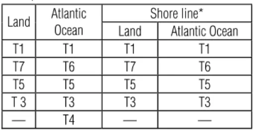
Table 1 – Types of cloud identification tests during day time period.
Tabela 1 –Tipos de testes para identificac¸˜ao de nuvens du-rante o per´ıodo diurno.
Shore line* Land Atlantic
Ocean Land Atlantic Ocean
T1 T1 T1 T1
T7 T6 T7 T6
T5 T5 T5 T5
T 3 T3 T3 T3
— T4 — —
*The identification of the pixel’s surface coverage (land, ocean) is determined by a test using AVHRR channels 1 and 2.
Table 2 – Types of cloud identification tests during night time period. Tabela 2 –Tipos de testes para identificac¸˜ao de nuvens durante o per´ıodo no-turno.
Atlantic Ocean Land and Shore line Without 3.7 µm channel With 3.7µm channel Without 3.7 µm channel With 3.7 µm channel T1 T1 T1 T1 T4 T2 T5 T2 T5 T3 — T3 .or. Within desert — T4 — Desert .or. T3 (desert’s limit) .or. T5 (Desert´s limit) — T5 — T5 RESULTS
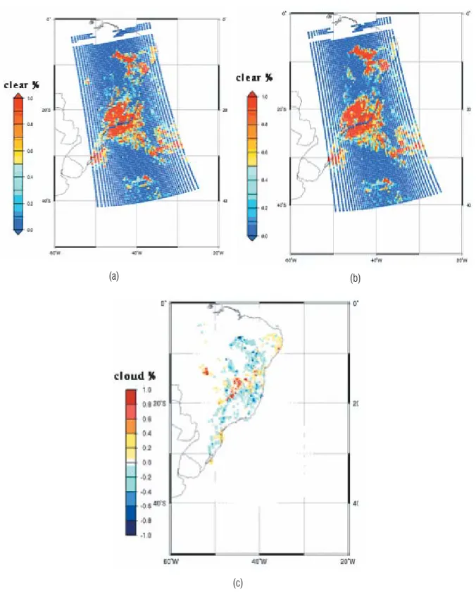
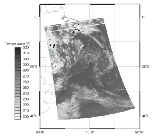
Figures 1a-b show the cloud coverage fraction from the NOAA-15 image on March 02, 2000 (night time) using the cloud mask algorithm. The pixels associated with cloud free sky are shown in red and those associated with overcast sky, in blue. The com-parison between the cloud masks algorithms (Figures 1a-b) and the corresponding 12.0µm infrared cloud cover image (Figure 2) showed a good agreement. The areas identified as cloud free by the cloud masks corresponded very well to those with high bright-ness temperature values in the 12.0µm image. On the other hand, the areas considered cloudy corresponded to the relatively low brightness temperature values.
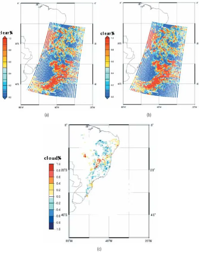
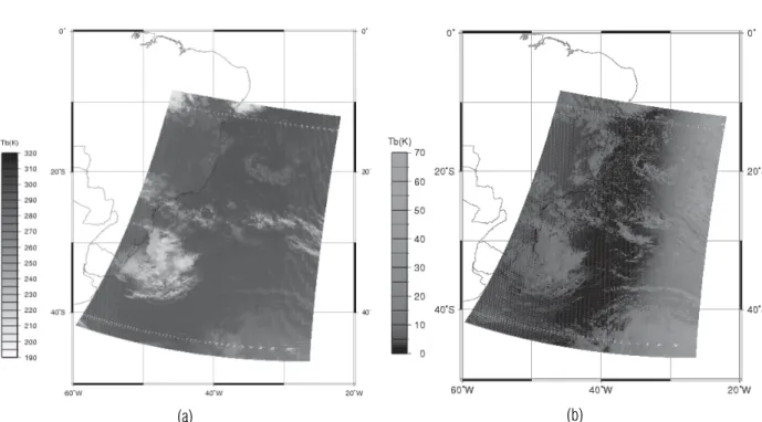
Figures 3a-b show the cloud masks for the February 23, day-time image, and Figure 4a, the corresponding infrared image. In this case, the visible image (Figure 4b) may be used to help the validation process for the cloud mask once the albedo values, as-sociated with different types of targets in the image, are known. Clouds normally have higher reflectivity indices, relatively to the typical Earth’s surface albedo and, therefore, areas with high al-bedo values must be associated with pixels total or partially con-taminated by clouds. On the other hand, areas with low albedo values are associated with pixels related to short wave radiation reflected by the surface, that is, cloud free regions. It is worth mentioning that for, some targets such as snow or sand covered (deserts) areas, the albedo is also very high and caution should be taken to avoid erroneously interpret them as clouds. In general, a good agreement was observed between the cloud masks and the infrared and visible images.
For the two cases analysed, the comparison between the re-sults obtained by the two versions of MAIA model indicated that regions identified as cloud free are practically the same in both versions and the differences between them are small, with the F version being slightly more inflexible; as a consequence, a large number of pixels were considered cloudy. This feature can also be observed in Figures 1c and 3c, that show the differences between F and C data versions, respectively for February 22 and March 02, 2000. Both versions show similar results over ocean areas, but they appear to overestimate cloud pixels, that is, some clear pixels may be being classified as cloud pixels.
Tables 3 and 4 show the fraction of pixels considered cloudy in each test used for cloud identification for the two cases previ-ously discussed. Only AVHRR pixels located within the bounds of an ellipsis formed by the HIRS FOV pixels were taken into ac-count in the calculations. A noticeable fraction difference in the pixel considered cloudy by the two versions was observed over land.
The use of forecast surface temperature allows for a more re-alistic threshold for the 11.0µm brightness temperature, above which a pixel is considered cloud. However, this threshold va-lue should be as small as possible, but large enough to take into account factors such as forecast errors, differences between the air temperature near the surface and surface radiometric tempera-ture, radiative cooling (night-time) or heating (day-time), surface emissivity, time differences between AVHRR observations and fo-recast times. In this study, for comparison purposes between C and F data versions, a threshold of 11K and 9K were adopted for the night and day time passages, respectively. It was also noti-ced that, when the forecast surface temperature version was used,
(a) (b)
(c)
Figure 1 – Fraction (%) of cloud coverage within HIRS FOV from NOAA-15 image of March 02, 2000 at 22:26 UTC: (a) F version (b) C version and (c) F - C. Figura 1 –Frac¸˜ao (%) da cobertura de nuvens dentro do FOV do HIRS da imagem do sat´elite NOAA-15, dia 02 de Marc¸o de 2000 `as 22:26 UTC: (a) vers˜ao F, (b) vers˜ao C e (c) F-C.
Figure 2 – Brightness temperature (K) derived from 12µm AVHRR infrared channel, on March 02, 2000 at 22:26 UTC. Figura 2– Temperatura de Brilho (K) derivada do canal infravermelho(12µm)AVHRR, dia 02 de marc¸o de 2000, `as 22:26 UTC.
a larger number of pixels was classified as cloudy over land ac-cording to T1 (not shown). However, over ocean areas the use of forecasted surface temperature did not influence the percent of pi-xels considered cloudy, or in other words, a climatological atlas of sea surface temperature could alternatively be used. This is pro-bably due to the smaller variability of the sea surface temperature, relatively to continental surfaces. Regarding other tests, the only difference between F and C data versions was in the amount of precipitable water. The use of climatological PW may yield large errors mainly the tropics where the moisture content in general is highly variable. On the other hand, the tests showed little sensi-tivity regarding the PW fields, except for T5, which presented a large percent reduction in cloudy pixels in the F data version. The results remained unchanged over ocean areas because the PW variable was the same in both versions.
It was also verified that the classical test for the temperature threshold (test T1) was the most reliable in identifying pixels sor-ted out as cloudy according to MAIA algorithm, although a con-siderable portion of these pixels was also identified by the other
tests. Regarding the night-time orbits, in addition to the threshold test T1, other tests (which classify a large number of pixels) were deemed important, such as test T4 (spatial coherence technique) and 2 (Tb3.7µm- Tb12µm). On the other hand, regarding the day-time passages, the most significant tests were T4 and T7 (not shown). Test T5 thatper seclassified a large amount of cloudy pixels hardly affects the final result of the cloud masks, that is, it was practically redundant for the analysed cases.
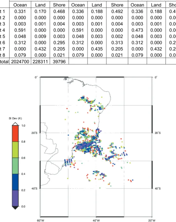
Test T4, as mentioned before, is based on the calculation of the brightness temperature standard deviation using pixels within a 3× 3 pixel “box”. A threshold of 0.2K is used as the maximum value allowed for the standard deviation in order to classify a pixel as cloud free. However, a more detailed analysis of the results for ocean areas showed that this value is not adequate for the region under consideration and that higher values, about 0.5K, could be used without compromising the reliability of the algorithm (pre-venting that cloud pixels be classified as cloud free ones). Figures 5 and 6 show the standard deviation average values for each HIRS pixel.
(a) (b)
(c)
Figure 3 – As in Figure 1, except for February 23, 2000 and 10:02 UTC. Figura 3 –Igual `a Figura 1,exceto para 23 de Fevereiro de 2000 e 10:02 UTC.
(a) (b)
Figure 4 – NOAA-15 AVHRR images on February 23, 2000 at 10:02 UTC: (a) brightness temperature (K), at 12.0µm (b) albedo at 0.6 µm. Figura 4 –Imagens NOAA-15 AVHRR para 23 de Fevereiro de 2000, `as 10:02 UTC: (a) temperatura de brilho (K) em 12.0µm (b) albedo em 0.6µm.
Table 3 – Fraction of pixels identified as cloudy by each test used by the cloud mask algorithm, for day 02/03/2000 at 22:26 UTC.
Tabela 3– Frac¸˜ao de pixels identificados como nublados por cada teste usado pelo algoritmo de m´ascara de nuvens para o dia 02/03/2000 `as 22:26 UTC.
C version F version STDEV version
Ocean Land Shore Ocean Land Shore Ocean Land Shore
Test 1 0.585 0.530 0.290 0.583 0.639 0.426 0.583 0.639 0.426 Test 2 0.399 0.669 0.367 0.399 0.619 0.343 0.399 0.619 0.343 Test 3 0.024 0.000 0.000 0.024 0.000 0.000 0.024 0.000 0.000 Test 4 0.798 0.000 0.000 0.798 0.000 0.000 0.713 0.000 0.000 Test 5 0.118 0.409 0.144 0.118 0.238 0.144 0.118 0.238 0.144 Pixel total 1340582 989214 54183
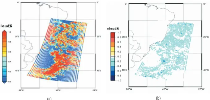
Franc¸a and Cracknell (1995) in their study on the Brazilian Northeast used for the standard deviation method a value of 0.4K, below which the pixel was classified as cloud free. This value was tested for the above-presented cases and the results are shown in Figures 7a and 8a. When the “STDEV” version of the cloud masks is checked against the forecast data version (Figures 1a and 3a), it is clear that the number of pixels given as cloudy is significan-tly reduced. This can also be seen in the graph that depicts the difference between the two versions (Figures 7b e 8b). The per-centage reduction in cloud pixels over the Atlantic Ocean occurred practically all over the image, with values ranging from 0 to 40%. Table 5 shows the pixel percent (with respect to the total image
pixel) that were considered cloud free according to test T4 and the final percent of these pixels (after the application of the sequence of tests) for the forecast data version as well for the version that utilizes the value of 0.4K for the standard deviation. In both cases a considerable reduction in cloud pixels was evident according to T4, which ended up also influencing the final cloud masks results.
CONCLUDING REMARKS
The results of this study show that the application of the cloud mask algorithm MAIA over Brazil showed that both versions of the algorithm (forecast and climatological data) produced similar results for the region under consideration, mainly over the ocean,
Table 4 – As Table 1, except for day 23/02/2000 and 10:02 UTC. Tabela 4– Igual `a Tabela 1,exceto para o dia 23/02/2000 e 10:02 UTC.
C version F version STDEV version
Ocean Land Shore Ocean Land Shore Ocean Land Shore Test 1 0.331 0.170 0.468 0.336 0.188 0.492 0.336 0.188 0.492 Test 2 0.000 0.000 0.000 0.000 0.000 0.000 0.000 0.000 0.000 Test 3 0.003 0.001 0.004 0.003 0.001 0.004 0.003 0.001 0.004 Test 4 0.591 0.000 0.000 0.591 0.000 0.000 0.473 0.000 0.000 Test 5 0.048 0.009 0.003 0.048 0.003 0.002 0.048 0.003 0.002 Test 6 0.312 0.000 0.295 0.312 0.000 0.313 0.312 0.000 0.295 Test 7 0.000 0.432 0.205 0.000 0.435 0.205 0.000 0.432 0.205 Test 8 0.079 0.000 0.021 0.079 0.000 0.021 0.079 0.000 0.021 Pixel total 2024700 228311 39796
Figure 5 – Standard deviation estimates (test T4) for each area within a 3× 3 pixel from NOAA 15 image on March 02, 2000 at 22:26 UTC.
Figura 5– Estimativas do desvio padr˜ao (teste T4) para cada ´area dentro de um pixel3× 3da imagem NOAA 15 do dia 02 de marc¸o de 2000 `as 22:26 UTC.
where they were identical, suggesting that the utilization of fore-cast data is not an impairment to a satisfactory classification using the cloud mask technique. However, this technique is sensitive to the value used in calculating the standard deviation for the
bright-ness temperature over the ocean, where a more appropriate value of 0.4K is suggested. It is important to mention that the compari-son problem, using outputs of cloud mask algorithm, is very dif-ficult because some types of clouds may be transparent in certain
Figure 6 – Standard deviation estimates (test T4) for each area within a 3× 3 pixel from NOAA 15 image on February 23, 2000 at 10:02 UTC. Figura 6– Igual `a Figura 5, exceto para dia 23 de Fevereiro de 2000 `as 10:02 UTC.
Table 5 – Pixel percent (with respect to the total image pixel) that were considered cloud free according to test T4 and the final percent of these pixels (after the application of the sequence of tests) for the F and STDEV version.
Tabela 5– Porcentagem de pixels (com relac¸˜ao ao total) que foram considerados como n˜ao nublados de acordo com o teste T4 e a porcentagem final desses pixels (ap´os a aplicac¸˜ao da seq¨uˆencia de testes) utilizando-se as vers˜oes F e STDEV.
F version
STDEV version
Analysed cases
Free cloud pixels
(Test T4)
Free cloud pixels
(Total)
Free cloud pixels
(Test T4)
Free cloud pixels
(Total)
02/03/2000 20.2%
17.9%
28.7%
23.1%
(a) (b)
Figure 7 – Fraction (%) of cloud coverage within HIRS field of view from NOAA-15 image of February 23, 2000 at 10:02 UTC: (a) using F version data with a new threshold for T4. (b) F-STDEV.
Figura 7 –Frac¸˜ao de cobertura de nuvens dentro do campo de visada do sensor HIRS processada a partir da imagem recebida do NOAA-15, dia 23/02/2000 `as 10:02 UTC: (a) utilizando dados de Previs˜ao com o novo limite para o teste T4; (b) diferenc¸a entre as vers˜oes Previs˜ao e STDEV.
(a) (b)
Figure 8 – As in Figure 7, but for March 02, 2000 at 22:26 UTC.
channels and the associated image may not reveal where these clouds are present. Also the current analyses focused only typical austral summer cases, thus, the obtained results are not definitive and complete.
REFERENCES
AAPP DOCUMENTATION. 1999. General specifications for the AAPP pre-processing package related to NOAA polar orbiting weather satellites. Scientific Part.
CARVALHO JC, RAMOS FM, FERREIRA NJ & CAMPOS VELHO HF. 1999. Retrieval of vertical temperature profiles in the atmosphere. Third Interna-tional Conference on Inverse Problems in Engineering, Port Ludlow, USA. CARVALHO JC. 2002. Modelagem e an´alise de sondagens remotas sobre o Brasil utilizando-se o sistema ICI. 0. 218.f: (Doutorado em Meteorolo-gia), Instituto Nacional de Pesquisas Espaciais, S˜ao Jos´e dos Campos, Brasil.
CHABOUREAU JP, CH´EDIN A & SCOTT NA. 1998. Remote sensing of the vertical distribution of the atmospheric water vapor from the TOVS observations: Method and validation. J. Geophys. Res., Washington, 103: 8743–8752.
EYRE JR, BROWNSCOMBE JL & ALLAM RJ. 1984. Detection of fog at night using advanced very high resolution radiometer (AVHRR) imagery. Meteor. Magazine, 113: 266–275.
ENGLISH SJ, JONES DC, DIBBEN PC, RENSHAW RJ & EYRE JR. 1999. The impact of cloud and precipitation on ATOVS soundings. ECMWF Report.
FRANC¸A GB & CRACKNELL AP. 1995. AVHRR daytime data masking approach using NOAA AVHRR daytime data for tropical areas. Int. J. R. Sens., 16(9): 1697–1705.
GRODY N, WENG F & FERRARO R. 1999. Application of AMSU for obtai-ning water vapour, cloud liquid water, precipitation, snow cover and sea ice concentration. Technical Proceedings of the Tenth International TOVS Study Conference, Boulder, Colorado.
LAVANANT L, BRUNEL P, ROCHARD G, LABROT T & POCHIC D. 1997. Current Status for the ICI Retrieval Scheme. Technical Proceedings of the Ninth International TOVS Study Conference, Igls, Austria, Feb.
LAVANANT L et al. (07 co-authors). 1999. AVHRR Cloud Mask for Soun-ding Applications. ITSC-10 proceeSoun-dings.
MAIA DOCUMENTATION. 1999. Mask AVHRR for inversion ATOVS. Sci-entific Part.
NOGUEIRA JLM. 1998. Impacto das imagens AVHRR na classificac¸˜ao de padr˜oes de nebulosidade utilizando o modelo ITPP5. 0. 75.f: (Mestrado em sensoriamento remoto), Instituto Nacional de Pesquisas Espaciais, S˜ao Jos´e dos Campos, Brasil.
SMITH WL, WOOLF HM & SCHRIENER AJ. 1985. Simultaneous retrie-val of surface and atmospheric parameters: a physical analytically direct approach. Advances in Remote Sensing, A. Deepak, H. E. Fleming and M. T. Chahine (Eds.), 7: 221–232.
SMITH WL. 1991. Atmospheric Soundings from satellite – false expec-tation or the key to improved weather prediction? Q.J.R. Meteorol. Soc., 117: 267–297.
SMITH WL, WOOLF HM, NIEMAN SJ & ACTHOR TH. 1993. ITPP-5 – the use of AVHRR and TIGR in TOVS data processing. Technical Procee-dings of the Seventh International TOVS Study Conference, Igls, Austria, Feb.
STUBENRAUCH CJ, ROSSOW WB, CH´ERUY F, CH´EDIN A & SCOTT NA. 1999a. Clouds as seen by satellite sounders (3I) and imagers (ISCCP). Part I: Evaluation of Cloud Parameters. J. Clim., Boston, 12(8): 2189– 2213.
STUBENRAUCH CJ, CH´EDIN A, ARMANTE R, SCOTT NA. 1999b. Clouds as seen by satellite sounders (3I) and imagers (ISCCP). Part II: A New Ap-proach for Cloud Parameter Determination in the 3I Algorithms. J. Clim., Boston, 12(8): 2214–2223.
NOTES ABOUT THE AUTHORS
Nelson Jesus Ferreira is a Senior Researcher of the Centro de Previs˜ao de Tempos e Estudos Clim´aticos (CPTEC), at Instituto Nacional de Pesquisas Espaciais-INPE, S˜ao Jos´e dos Campos, SP, Brazil. He has a degree in Physics and a MSc in Meteorology from INPE and a PhD in Meteorology from the University of Wisconsin-Madison, EUA. His research interests are Remote Sensing of the Atmosphere and Synoptic Meteorology.
Jo˜ao Carlos Carvalho has a degree in Physics from the Universidade Federal de S˜ao Carlos, UFSCar and a MSc and Doctor degree in Meteorology from the Instituto Nacional de Pesquisas Espaciais, INPE. Currently he is working for the Hidrology Team of the Remote Sensing Division, INPE.
Fernando Manuel Ramos is a Senior Researcher of Computation and Aplied Matematics Laboratory, at Instituto Nacional de Pesquisas Espaciais-INPE, S˜ao Jos´e dos Campos, SP, Brazil. He has a degree in Mechanical-Aeronautical Engineering from the Instituto Tecnol´ogico de Aeron´autica, ITA and a MSc in Space Sciences from INPE and a PhD in Fluid Mechanics from the ENSAE, France. His research interests are inverse and ill-posed problems, numerical heat transfer, spacecraft thermal testing and design and applied meteorology.