Characterization of the sulphate mineral coquimbite, a secondary iron sulphate from Javier Ortega mine, Lucanas Province, Peru – Using infrared, Raman spectroscopy and thermogravimetry

(1)

Characterization of the sulphate mineral coquimbite, a secondary iron

sulphate from Javier Ortega mine, Lucanas Province, Peru – Using

infrared, Raman spectroscopy and thermogravimetry

Ray L. Frost

a,_⇑

_{, Zˇeljka Zˇigovecˇki Gobac}

b

_{, Andrés López}

a

_{, Yunfei Xi}

a

_{, Ricardo Scholz}

c

_{, Cristiano Lana}

c

_,

Rosa Malena Fernandes Lima

d

a_{School of Chemistry, Physics and Mechanical Engineering, Science and Engineering Faculty, Queensland University of Technology, GPO Box 2434, Brisbane, Queensland 4001, Australia} b

Institute of Mineralogy and Petrography, Department of Geology, Faculty of Science, University of Zagreb, Horvatovac 95, 10000 Zagreb, Croatia c

Geology Department, School of Mines, Federal University of Ouro Preto, Campus Morro do Cruzeiro, Ouro Preto, MG 35400-00, Brazil d

Mining Engineering Department, School of Mines, Federal University of Ouro Preto, Campus Morro do Cruzeiro, Ouro Preto, MG 35400-00, Brazil

h i g h l i g h t s

We have studied the mineral coquimbite.

Using SEM with EDX, thermal analytical techniques and Raman and infrared spectroscopy. Chemical formula was determined asðFe3þ

1:37;Al0:63ÞP2:00ðSO4Þ39H2O.

Thermal analysis showed a total mass loss of73.4% on heating to 1000°C.

a r t i c l e

i n f o

Article history:

Received 19 November 2013

Received in revised form 30 January 2014 Accepted 30 January 2014

Available online 3 February 2014

Keywords:

Coquimbite Amarantite Raman spectroscopy Sulphate

Infrared spectroscopy

a b s t r a c t

The mineral coquimbite has been analysed using a range of techniques including SEM with EDX, thermal analytical techniques and Raman and infrared spectroscopy. The mineral originated from the Javier Ortega mine, Lucanas Province, Peru. The chemical formula was determined asðFe3þ

1:37;Al0:63ÞP_2:00ðSO4Þ₃9H2O. Thermal analysis showed a total mass loss of73.4% on heating to 1000°C. A mass loss of 30.43% at

641.4°C is attributed to the loss of SO3. Observed Raman and infrared bands were assigned to the stretching and bending vibrations of sulphate tetrahedra, aluminium oxide/hydroxide octahedra, water molecules and hydroxyl ions. The Raman spectrum shows well resolved bands at 2994, 3176, 3327, 3422 and 3580 cm1_{attributed to water stretching vibrations. Vibrational spectroscopy combined with} thermal analysis provides insight into the structure of coquimbite.

1. Introduction

Coquimbite is an iron (III) sulphate mineral of ideal formula Fe3þ

2 ðSO4Þ39H2O, which derives its name from the Coquimbo re-gion, Chile[1]. Coquimbite is found as secondary mineral devel-oped in the oxidized portions of weathering iron sulphide deposits in arid regions, although it could be also found associated with fumarolic activity[1]. The mineral was first described from Tierra Amarilla near Copiapó, Chile[2–5], and other occurrences were reported in Quetena, Chuquicamata, Alcaparrosa, Chile; Con-cepción mine, Huelva, Spain; Skouriotisa, Cyprus; Rammelsberg, Hartz, Germany, among others[1,3,6–8].

Coquimbite was recently found in Peru, at the Javier Ortega mine, Lucanas Province, Departmento Ayacucho[9]. Main ore min-eral in Javier Ortega mine is chalcopyrite and secondary ore miner-als are sphalerite and galena[9]. Coquimbite occurs in the oxidized portions of this iron sulphide deposit, together with other second-ary sulphate minerals like alunogen, chalcanthite, copiapite, halo-trichite, jarosite, krausite, römerite and with sulphur. Coquimbite in Javier Ortega mine occurs in well developed violet crystals up to 5 cm long[9].

Coquimbite is a hexagonal mineral[10,11]witha= 10.922(9), c= 17.084(14) Å, space groupP31 c andZ= 4 [12]. Ideal formula of this mineral is Fe3þ

2 ðSO4Þ39H2O, but there is often a replace-ment of Fe3+_{by Al}3+_{, so the formula of this mineral should be} writ-ten Fe3þ

2xAlxðSO4Þ39H2O [6,12]. There are three outstanding features of the coquimbite structure. The dominant structural

⇑ Corresponding author. Tel.: +61 731382407; fax: +61 731381804.

E-mail address:r.frost@qut.edu.au(R.L. Frost).

Contents lists available atScienceDirect

Journal of Molecular Structure

(2)

feature is a discontinuous chain, composed of alternating Fe octa-hedra and S tetraocta-hedra, parallel to, and approximately one-half the length of, thecaxis. The symmetry causes the chain to be repeated in the upper one-half of the cell. The individual chain segments (i.e. two centrosymmetrically related clusters of six SO4tetrahedra and three Fe octahedra in each unit cell) are linked through hydrogen bonds only. The second structural feature is the geometrical arrangement of these chains which gives rise to ‘‘channels’’, paral-leling thea1anda2axes, which are occupied by water molecules

linked to the chains by hydrogen bonds. The third structural fea-ture are independent (Al, Fe) octahedra located at the origin and at the centre of thecedges surrounded by six H2O molecules. There are three crystallographically different iron atoms octahedrally coordinated to six O and/or Ow (= oxygen atom of an H2O mole-cule) forming Fe1O46, Fe2O33Ow33, and Fe3Ow16octahedra. Two of in total three crystallographically independent H2O molecules, Ow1 and Ow3 are bonded to one iron atom, whereas Ow2 is not bonded to any cation. The meanhFe–Oidistance of Fe3 site differ

from distances of Fe1 and Fe2 sites, and such a difference in aver-age bond distance can be attributed to the partial Fe3 site occupa-tion also by Al atoms. So, the crystal structure of coquimbite could be described as a [Fe4(H2O)12(SO4)6]0 _{framework consisting of} [Fe1Fe22(H2O)6(SO4)6]3_{clusters and isolated [Fe3(H2O)6]}3+ octa-hedra connected to each other only by hydrogen bonds. Ow1 and Ow3 atoms are engaged in the further interconnection of the [Fe3-Ow36(SO4)6] clusters and [FeOw16] octahedra. And Ow2 atoms which build hydrogen-network-bonded H2O molecules (H2Ow2) which are placed in channels running parallel to thea axis (in cages made by channel’s intersection) occupy positions which can be compared to the corners of a flattened octahedron and there can be distinguished two bonding-scheme types for this Ow2 atoms, i.e. two hydrogen-bonded network variants around the H2Ow2 molecules[13].

Rietveld refinement of the coquimbite structure[14]on a sam-ple from the Richmond mine, Redding, California, proved that there is, together with the Al-for-Fe substitution on Fe3 site, also a minor Al-for-Fe substitution on the Fe1 site. Although there is a possibil-ity of a wide range of continuous replacement of the Fe3+_{by other} ions of similar radius, such as especially aluminium, without modifying the structural type, on increasing the Al content beyond a certain limit, a structural rearrangement of the phase occurs, leading to the new mineral species aluminocoquimbite AlFe3+_(SO4)3

9H2O[15–17]. Mineral coquimbite is polytypic with

paracoquimbite, a rhombohedral mineral (space group R3) [18]. These two minerals, i.e. two layer-like crystal structures differ in layer stacking sequences, with a repeat distance of 8.5 Å between structurally identical but spatially transposed layers.

Approximately 370 sulphate-mineral species are known to exist in nature and they are found in a variety of geological settings, including volcanic, hydrothermal, evaporitic, and chemical-weath-ering environments[19]. A problem in identification of such min-erals with techniques like an X-ray diffraction arrives when closely related minerals are found in paragenetic relationship [20]. So, vibrational spectroscopic techniques are applicable in identifica-tion of such paragenetically related minerals.

2. Experimental procedure

2.1. Samples description and preparation

The mineral coquimbite studied in this work was obtained from the collection of the Geology Department of the Federal University of Ouro Preto, Minas Gerais, Brazil, with sample code SAB-101. The sample is from the Javier Ortega mine, Lucanas Province, Peru.

The sample was gently crushed and the associated minerals were removed under a stereomicroscope Leica MZ4. The coquim-bite sample was phase analysed by X-ray diffraction. Scanning electron microscopy (SEM) was applied to support the mineralog-ical chemmineralog-ical.

2.2. Scanning electron microscopy (SEM)

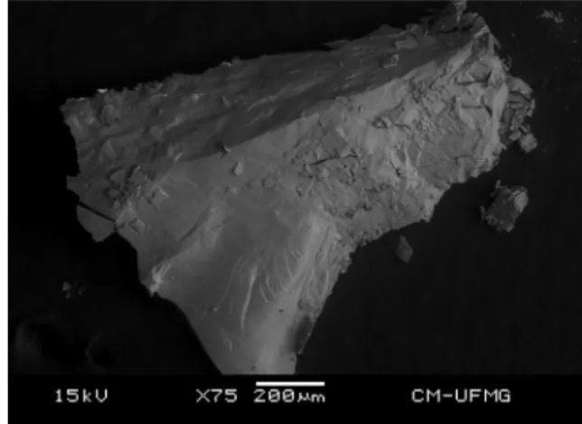
Coquimbite cleavage fragments were coated with a 5 nm layer of evaporated Au. Secondary Electron and Backscattering Electron

Fig. 1.Backscattered electron image (BSI) of a coquimbite crystal aggregate up to 0.5 mm in length.

Fig. 2.EDS analysis of coquimbite.

(3)

images were obtained using a JEOL JSM-6360LV equipment. Qual-itative and semi-quantQual-itative chemical analyses in the EDS mode were performed with a ThermoNORAN spectrometer model Quest and were applied to support the mineral characterization.

2.3. Thermogravimetric analysis – TG/DTG

Thermogravimetric analysis of the coquimbite mineral were ob-tained by using TA Instruments Inc. Q50 high-resolution TGA oper-ating at a 10°C/min ramp with data sample interval of 0.50 s/pt from room temperature to 1000°C in a high-purity flowing nitro-gen atmosphere (100 cm3_{/min). A mass of about 28.0 mg of finely} ground dried sample was heated in an open platinum crucible.

2.4. Raman spectroscopy

Crystals of coquimbite were placed on a polished metal surface on the stage of an Olympus BHSM microscope, which is equipped with 10, 20, and 50 objectives. The microscope is part of a Renishaw 1000 Raman microscope system, which also includes a monochromator, a filter system and a CCD detector (1024 pixels). The Raman spectra were excited by a Spectra-Physics model 127 He–Ne laser producing highly polarised light at 633 nm and col-lected at a nominal resolution of 2 cm1 _{and a precision of}

Fig. 4.(a) Raman spectrum of coquimbite (upper spectrum) over the 100–4000 cm1_{spectral range and (b) infrared spectrum of coquimbite (lower spectrum) over the 500–}

4000 cm1_{spectral range.}

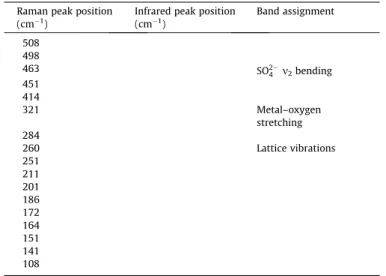
Table 1

Table of the Raman and infrared bands and their assignments.

Raman peak position (cm1₎

Infrared peak position (cm1₎

Band assignment

3580 3678 OH stretching

3422 3536

3327 3424 Water stretching

3176 3288

2994 3096

1661 1651 Water bending

1201 1172 SO2

4 m₃

1165 1161 Antisymmetric

stretching

1113 1100

1095 1060

1037

1025 1024 SO2

4 m₁symmetric

stretching

1015 1011

1002

942 Water librational 828

673 701

620 668

599

525 SO2

4 m₄bending

(4)

±1 cm1_{in the range between 200 and 4000 cm}1_{. Repeated} acqui-sitions on the crystals using the highest magnification (50) were

accumulated to improve the signal to noise ratio of the spectra. Raman Spectra were calibrated using the 520.5 cm1 _{line of a}

silicon wafer. The Raman spectrum of at least 10 crystals was collected to ensure the consistency of the spectra.

2.5. Infrared spectroscopy

Infrared spectra were obtained using a Nicolet Nexus 870 FTIR spectrometer with a smart endurance single bounce diamond ATR cell. Spectra over the 4000–525 cm1 _{range were obtained} by the co-addition of 128 scans with a resolution of 4 cm1_{and a} mirror velocity of 0.6329 cm/s. Spectra were co-added to improve the signal to noise ratio.

Spectral manipulation such as baseline correction/adjustment and smoothing were performed using the Spectracalc software package GRAMS (Galactic Industries Corporation, NH, USA). Band component analysis was undertaken using the Jandel ‘Peakfit’ soft-ware package that enabled the type of fitting function to be se-lected and allows specific parameters to be fixed or varied accordingly. Band fitting was done using a Lorentzian-Gaussian cross-product function with the minimum number of component bands used for the fitting process. The Gaussian–Lorentzian ratio was maintained at values greater than 0.7 and fitting was under-taken until reproducible results were obtained with squared corre-lations ofr2greater than 0.995.

Fig. 5.(a) Raman spectrum of coquimbite (upper spectrum) in the 800–1300 cm1_{spectral range and (b) infrared spectrum of coquimbite (lower spectrum) in the 500–}

Table 1(continued)

Raman peak position (cm1₎

Infrared peak position (cm1₎

Band assignment

508 498

463 SO2

4 m₂bending

451 414

321 Metal–oxygen

stretching 284

260 Lattice vibrations

251 211 201 186 172 164 151 141 108

(5)

3. Results and discussion

3.1. Chemical characterization

The BSI image of coquimbite sample studied in this work is shown inFig. 1. Qualitative and semi-quantitative chemical com-position shows a Fe and Al sulphate phase. The chemical analysis is represented as an EDS spectrum in Fig. 2. On the basis of semiquantitative chemical analyses the chemical formula was calculated asðFe3þ

1:37;Al0:63ÞP2

:00ðSO4Þ39H2O.

3.2. Thermal analysis

The thermal analysis of coquimbite is illustrated in Fig. 3. To date, there have been no thermal analytical studies of coquimbite and related minerals[21,22]. There have been some differential thermal analysis study of a very wide range of sulphates from some years past[23]. The TG curve shows a total mass loss of73.4% on heating to 1000°C and is in agreement with the stoichiometric content of H2O and SO3that correspond to 74.0 wt%. A significant number of decomposition steps are observed according to the DTG curve in Fig. 3. Small mass loss steps are found at 37, 48 and 94°C. These mass los steps may be attributed to the loss of

adsorbed water. Further mass loss steps are observed at 135, 161, 254 and 262°C. These mass loss steps are assigned to the loss of water in stages. Two minor mass losses are found at 393 and 546°C. A very large mass loss occurs at 695°C and is assigned to the mass loss of SO3due to sulphate decomposition. The total mass loss of water according to the given formula is 34.76% and the mass loss of sulphate as SO3 equals 34.73%. Thus the theoretical total mass loss is 69.5%. Thus the difference between the theoretical mass loss and the observed mass loss is 3.9% which is attributed to the loss of adsorbed water.

In the temperature range of 25–100°C, is observed a mass loss of about 5.2%. The accepted formula by the IMA is Fe3þ

2 ðSO4Þ39H2O. This mass loss is attributed to the loss of ad-sorbed water, according to the equation:

Fe3þ

2 ðSO4Þ39H2O!Fe

3þ

2 ðSO4Þ39H2OþH2O

In the temperature range of 500–700°C a mass loss of 30.43%. A strong exothermic reaction is observed at 641.4°C. This mass loss is attributed to the loss of sulphate.

Fe3+_(SO4)3

?Fe2O3+ SO3. According to this reaction the mass loss of 36% would be predicted based upon the formula Fe3þ

2 ðSO4Þ39H2O. A mass loss of 30.43% is observed for this step.

Fig. 6.(a) Raman spectrum of coquimbite (upper spectrum) in the 300–800 cm1_{spectral range and (b) Raman spectrum of coquimbite (lower spectrum) in the 100–}

(6)

3.3. Vibrational spectroscopy

Coquimbite as well as other iron sulphate minerals, were al-ready investigated using NIR spectroscopy[20]and mid-infrared emission spectroscopy [24]. For NIR 6400–7400 cm1 _spectral region, spectrum of mineral coquimbite was characterized by overlap of the first HOH fundamentals and the HOH combination bands, and mineral showed intense bands at 6918 and 6646 cm1_{. In NIR 4000–5500 cm}1 _{spectral region, bands were} observed for coquimbite at 5214, 5144, 5066, 5010 and 4838 cm1_{. In the high wavenumber region (7500–1100 cm}1₎ iron (III) minerals, and so did coquimbite, showed no bands[20]. Early mid-infrared spectroscopic studies have shown that the aqueous sulphate anion (SO4)2_{produces four infrared absorption} features at1105,983,611, and450 cm1_{(corresponding to} the antisymmetric stretch,

m

3; symmetric stretch,

m

1; asymmetric bend,

m

4; symmetric bend

m

2, respectively) of which only

m

₃and

m

₄are infrared active[24,25]. These vibrations are modified when the sulphate anion is present within a solid-state medium, such as a mineral with a repeating molecular order, resulting in the poten-tial appearance of all four sulphate vibrational modes in the spec-trum [24]. In mid-infrared emission spectroscopy investigations, spectra of sample containing both, coquimbite and paracoquimbite showed two clear

m

₃features at 1180 and 1100 cm1; where the

shape of the 1100 cm1_{band suggested that there may be another} weaker

m

₃ band at slightly lower frequency. There were also a strong

m

₁feature present at 1013 cm1, three bands at 685, 650, and 975 cm1_{, and two}

_m

2 features at 480 and 443 cm1, with strong lattice modes occurring at <350 cm1_[24]_.

The Raman spectrum of coquimbite over the 100–4000 cm1 spectral range is reported inFig. 4a. This figure shows the position and relative intensity of each Raman band. The spectrum may be subdivided into sections depending upon the type of vibration being analysed. The infrared spectrum of coquimbite in the 500– 4000 cm1_{spectral region is illustrated in}_{Fig. 4}_{b. This spectrum} shows the position and relative intensity of the infrared bands. This spectrum may be subdivided into subsections based upon the vibrational spectroscopic region. The results of the Raman spectro-scopic analysis are summarised inTable 1. This Table shows the peak positions of the Raman and infrared bands and their assignment.

3.4. Raman spectroscopy in the 800–1400 cm1_{spectral range}

The Raman spectrum of coquimbite over the 800–1300 cm1 spectral range is provided inFig. 5a. The spectrum is dominated by an intense Raman band at 1025 cm1 _{and is assigned to the} SO2

4

m

1 symmetric stretching mode. Two shoulder bands are

(7)

observed at 1015 and 1037 cm1_{. Four low intensity bands} observed at 1095, 1113, 1165 and 1201 cm1 _{are attributed to} the SO2

4

m

3antisymmetric stretching modes.

3.5. Infrared spectroscopy in the 500–1300 cm1

spectral range

The infrared spectrum of coquimbite in the 500–1300 cm1 spectral range is given inFig. 5b. The spectrum shows complexity with a significant number of overlapping bands. The infrared bands recognised at 1060, 1100, 1161 and 1172 cm1_{are assigned to the} SO2

4

m

₃ antisymmetric stretching modes. The infrared bands at 1011 and 1024 cm1 _{are attributed to the SO}2

4

m

1 symmetric stretching mode.

3.6. Raman spectroscopy in the 300–800 cm1_{and in 100–300 cm}1

spectral ranges

The Raman spectrum of coquimbite in the 300–800 cm1 spec-tral range is shown inFig. 6a. The Raman spectrum in the 100– 300 cm1_{spectral range is provided in}_{Fig. 6}_{b. The complexity of} the antisymmetric stretching region is reflected in the spectra of the

m

₂bending region. A very intense Raman band is observed at 508 cm1 _{with additional Raman bands at 414, 451, 463 and}

498 cm1_{. These bands are assigned to the}

_m

2bending modes. Mul-tiple bands are observed in the 400–500 cm1 _{region for many} minerals and are attributed to the

m

₂bending modes. These multi-ple bands in this

m

₂spectral region are in harmony with the multi-ple bands observed in the

m

₃spectral region. These multiple bands may occur for several reasons one of which is the reduction of sym-metry of the sulphate anion and secondly the fact that not all the sulphate anions are equivalent in the coquimbite structure. A com-parison may be made with other sulphate bearing minerals. Bands are observed at 479, 443 and 408 cm1_{for cyanotrichite, at 450} and 430 cm1_{for devilline, 498 and 471 cm}1_{for glaucocerinite,} at 475, 445 and 421 cm1_{for serpierite and at 475 and 449 for} ktenasite. For the mineral amarantite, a very intense Raman band is observed at 409 cm1 _{with additional bands at 399, 451 and} 491 cm1_.

The Raman bands at 599, 621 and 673 cm1_{are assigned to the} sulphate

m

₄bending modes. The observation of multiple bands in this spectral region is in accordance with a reduction in symmetry of the sulphate anion in the coquimbite structure. A comparison may be made with the vibrational spectra of amarantite. A series of low intensity Raman bands for amarantite found at 543, 602, 622 and 650 cm1 _{are assigned to the}

_m

4 bending modes. The Raman spectrum of ktenasite shows a single peak in the

m

₄region

(8)

at 604 cm1_{. The Raman spectrum of devilline shows two low} intensity bands at 668 and 617 cm1_{; cynaotrichite two} overlap-ping bands at 594 and 530 cm1_{; the Raman spectrum of} glauco-cerinite shows two bands at 694, 613 and 555 cm1_{. The} complexity of the symmetric and antisymmetric bending region shows a reduction in symmetry for these complex sulphate minerals. Raman spectra of the mineral phases for this region are different, and each phase has its own characteristic spectrum. The observation of multiple bands supports the concept of a reduc-tion in symmetry of sulphate in the coquimbite structure. The Ra-man spectrum in the far low wavenumber region is shown in

Fig. 6b. An intense Raman band at 284 cm1_{is assigned to FeO} stretching vibrations. Other bands in this spectral region are sim-ply described as lattice vibrations.

The Raman spectrum of coquimbite over the 2600–3800 cm1 spectral range is displayed inFig. 7a. The infrared spectrum over this spectral range is given inFig. 7b. Both spectra are broad with several overlapping bands. The Raman spectrum shows well re-solved Raman bands at 2994, 3176, 3327, 3422 and 3580 cm1_. These bands are assigned to the water stretching vibrations. The bands are less well resolved in the infrared spectrum. Infrared bands are noted at 2758, 2924, 3096, 3288, 3424, 3536 and 3678 cm1_{. It is likely that the sharp Raman band at 3580 cm}1 is attributable to OH stretching vibrations.

The Raman spectrum of coquimbite over the 1300–2000 cm1 spectral range is shown inFig. 8a. This spectrum shows a broad Ra-man band at 1661 cm1_{. This band is assigned to the water} bend-ing mode. The position of this band supports the concept of very strongly hydrogen bonded water in the coquimbite structure. The position of the water bands in both the Raman and infrared spectra shows that water is strongly hydrogen bonded in the coquimbite structure. Raman and infrared bands below say 4000 cm1 _are indicative of strongly hydrogen bonded water. Bands above 3400 cm1 _{are indicative of weakly hydrogen bonded water in} the coquimbite structure.

4. Conclusions

The techniques of electron microscopy, thermogravimetry and vibrational spectroscopy have been combined to determine the chemistry of the mineral coquimbite. Chemical analysis using an electron probe shows qualitatively that only Fe and S are present. On the basis of semiquantitative chemical analyses, the chemical formula was calculated as (Fe3+_{1.37, Al0.63)}_P

2.00(SO4)39H2O. The TG curve shows a total mass loss of73.4% on heating to

1000°C in agreement with the stoichiometric content of H2O and SO3that correspond to 74.0 wt%.

Thermogravimetry proves the thermal decomposition of coquimbite takes place in a series of four major steps at 135,

161, 254 and 262°C. A very large mass loss occurs at 695°C and is assigned to the mass loss of SO3due to sulphate decomposition. Raman spectroscopy is a very powerful tool for the study of sul-phate minerals. In this work we have used vibrational spectroscopy to study the mineral coquimbite, a mineral found in evaporate deposits and land surfaces with extreme aridity. Multiple antisym-metric stretching bands are observed as well as multiple bending modes suggesting a reduction in symmetry of the sulphate in the coquimbite structure.

Acknowledgments

The financial and infra-structure support of the Queensland University of Technology, School of Chemistry, Physics and Mechanical Engineering is gratefully acknowledged. The Australian Research Council (ARC) is thanked for funding the instrumentation. The authors would like to acknowledge the Center of Microscopy at the Universidade Federal de Minas Gerais (http://www.microscopia. ufmg.br) for providing the equipment and technical support for experiments involving electron microscopy. R. Scholz thanks to CNPq – Conselho Nacional de Desenvolvimento Científico e Tecnológico (Grant No. 306287/2012-9 and No. 402852/2012-5). Zˇ. Zˇigovecˇki Gobac thanks to Ministry of Science, Education and Sports of the Republic of Croatia, under Grant No. 119-0000000-1158.

References

[1]J.W. Anthony, R.A. Bideaux, K.W. Bladh, M.C. Nichols, Handbook of Mineralogy,, vol. V, Borates, Carbonates, Sulfates., Mineral Data Publishing, Tucson, 2003. [2]H. Rose, Annal. Phys. Chem. 27 (1833) 309–319.

[3]J.F.A. Breithaupt, Arnoldische Buchhandlung, Dresden and Leipzig, 1841. [4]A. Arzruni, Zeit. Kryst. Min. 3 (1879) 516–524.

[5]G. Linck, Zeit. Kryst. Min. 15 (1889) 1–28.

[6] C. Palache, H. Berman, C. Frondel, Dana’s system of mineralogy, 7th edition ed., 1951.

[7]A. Kovacs, Foldtani Kozlony 127 (1998) 353–370. [8]J.H. Bernard, J. Hyršl, Granit, Prague, 2006. [9]J. Hyršl, Miner. Welt 3 (2010) 68–71.

[10]D.M.C. Huminicki, F.C. Hawthorne, Can. Min. 38 (2000) 1425–1432. [11]M. Mrose, D.E. Appleman, Zeit. Kryst. Min. 117 (1962) 16–36. [12]J.-H. Fang, P.D. Robinson, Am. Min. 55 (1970) 1534–1539.

[13]C. Giacovazzo, S. Menchetti, F. Scordari, Rendiconti 49 (1970) 129–140. [14]J. Majzlan, A. Navrotsky, R.B. McCleskey, C.N. Alpers, Eur. J. Min. 18 (2006)

175–186.

[15]F. Demartin, C. Castellano, C.M. Gramaccioli, I. Campostrini, Can. Min. 48 (2010) 323–333.

[16]F. Demartin, C. Castellano, C.M. Gramaccioli, I. Campostrini, Can. Min. 48 (2010) 1465–1468.

[17]F. Demartin, C. Castellano, C.M. Gramaccioli, I. Campostrini, Min. Mag. 74 (2010) 375–377.

[18]P.D. Robinson, J.H. Fang, Am. Min. 56 (1971) 1567–1572.

[19]F.C. Hawthorne, S.V. Krivovichev, P.C. Burns, The Crystal Chemistry of Sulfate Minerals, Sulfate Minerals: Crystallography, Geochemistry, and Environmental, significance ed., Mineralogical Society of America, Chantilly, Virginia, 2000.

[20]R.L. Frost, R.-A. Wills, W. Martens, M. Weier, B.J. Reddy, Spectrochim. Acta 62A (2005) 42–50.

[21]R. Scharizer, Zeit. Kryst. Min. 56 (1921) 353–385. [22]R. Scharizer, Zeit. Kryst. Min. 65 (1927) 335–360. [23]G. Cocco, Periodico di Min. 21 (1952) 103–138. [24]M.D. Lane, Am. Min. 92 (2007) 1–18.

[25]K. Nakamoto, Infrared and Raman Spectra of Inorganic and Coordination Compounds, Wiley & Sons, New York, 1986.