Universidade de Brasília
Instituto de Ciências ExatasDepartamento de Ciência da Computação
Characterization of Implied Scenarios as Families of
Common Behavior
Caio Batista de Melo
Dissertação apresentada como requisito parcial para conclusão do Mestrado em Informática
Orientadora
Prof.a Dr.a Genaína Nunes Rodrigues
Brasília
2018
Universidade de Brasília
Instituto de Ciências ExatasDepartamento de Ciência da Computação
Characterization of Implied Scenarios as Families of
Common Behavior
Caio Batista de Melo
Dissertação apresentada como requisito parcial para conclusão do Mestrado em Informática
Prof.a Dr.a Genaína Nunes Rodrigues (Orientadora) CIC/UnB
Prof. Dr. André Cançado Prof. Dr. George Teodoro
EST/UnB CIC/UnB
Prof. Dr. Bruno Luiggi Macchiavello Espinoza
Coordenador do Programa de Pós-graduação em Informática
Dedicatória
Dedico este trabalho a você que está lendo. Espero que este lhe ajude em seus próprios trabalhos e estudos, assim como muitos outros ajudaram para que este fosse concluído.
Agradecimentos
Aos meus professores, que me propiciaram a oportunidade de chegar até aqui, sempre contribuindo para o meu crescimento pessoal e profissional. Também aos meus amigos, que me acompanharam nesta caminhada onde criamos alegres lembranças. E principalmente à minha família, pelo constante apoio e por me colocar no caminho de grandes conquistas.
Resumo
Sistemas concorrentes enfrentam uma ameaça à sua confiabilidade em comportamentos emergentes, os quais não são incluídos na especificação, mas podem acontecer durante o tempo de execução. Quando sistemas concorrentes são modelados a base de cenários, é possível detectar estes comportamentos emergentes como cenários implícitos que, analo-gamente, são cenários inesperados que podem acontecer devido à natureza concorrente do sistema. Até agora, o processo de lidar com cenários implícitos pode exigir tempo e esforço significativos do usuário, pois eles são detectados e tratados um a um. Nesta dissertação, uma nova metodologia é proposta para lidar com vários cenários implícitos de cada vez, encontrando comportamentos comuns entre eles. Além disso, propomos uma nova maneira de agrupar estes comportamentos em famílias utilizando uma técnica de agrupamento usando o algoritmo de Smith-Waterman como uma medida de similaridade. Desta forma, permitimos a remoção de vários cenários implícitos com uma única correção, diminuindo o tempo e o esforço necessários para alcançar maior confiabilidade do sistema. Um total de 1798 cenários implícitos foram coletados em sete estudos de caso, dos quais 14 famílias de comportamentos comuns foram definidas. Consequentemente, apenas 14 restrições foram necessárias para resolver todos os cenários implícitos coletados coletados, aplicando nossa abordagem. Estes resultados suportam a validade e eficácia da nossa metodologia.
Palavras-chave: dependabilidade, cenários implícitos, sistemas concorrentes, LTSA,
Abstract
Concurrent systems face a threat to their reliability in emergent behaviors, which are not included in the specification but can happen during runtime. When concurrent systems are modeled in a scenario-based manner, it is possible to detect emergent behaviors as implied scenarios (ISs) which, analogously, are unexpected scenarios that can happen due to the concurrent nature of the system. Until now, the process of dealing with ISs can demand significant time and effort from the user, as they are detected and dealt with in a one by one basis. In this paper, a new methodology is proposed to deal with various ISs at a time, by finding Common Behaviors (CBs) among them. Additionally, we propose a novel way to group CBs into families utilizing a clustering technique using the Smith-Waterman algorithm as a similarity measure. Thus allowing the removal of multiple ISs with a single fix, decreasing the time and effort required to achieve higher system reliability. A total of 1798 ISs were collected across seven case studies, from which 14 families of CBs were defined. Consequently, only 14 constraints were needed to resolve all collected ISs, applying our approach. These results support the validity and effectiveness of our methodology.
Keywords: dependability, implied scenarios, concurrent systems, LTSA, Smith-Waterman,
Contents
1 Introduction 1
1.1 Context . . . 1
1.2 Problem . . . 2
1.3 Research Questions and Contributions . . . 2
1.4 Outline . . . 4
2 Background 5 2.1 Scenarios . . . 5
2.1.1 Message Sequence Chart . . . 6
2.1.2 Labeled Transition System . . . 8
Finite State Process Notation . . . 10
2.1.3 Implied Scenarios . . . 11 2.2 Clustering . . . 13 2.2.1 Hierarchical Clustering . . . 14 2.3 Smith-Waterman Algorithm . . . 17 3 Related Work 20 4 Methodology 24 4.1 Overview . . . 24 4.2 Detailed Steps . . . 26
4.2.1 Detecting Common Behaviors . . . 26
4.2.2 Classifying Families of Common Behaviors . . . 29
4.2.3 Treating Families of Common Behaviors . . . 30
4.3 Example . . . 34
4.3.1 Collecting Implied Scenarios . . . 34
4.3.2 Detecting Common Behaviors . . . 34
4.3.3 Classifying Families of Common Behaviors . . . 37
5 Evaluation 42
5.1 Setup . . . 42
5.2 Case Studies . . . 43
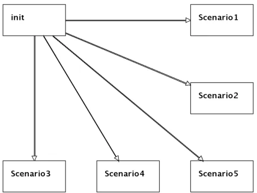
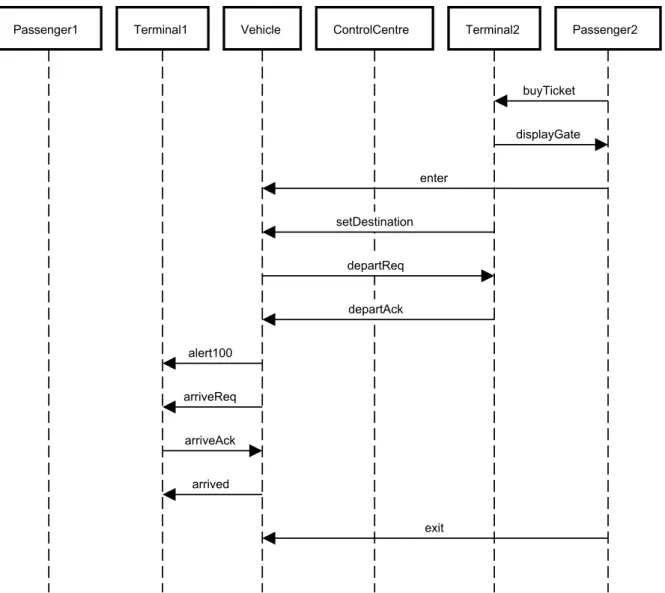
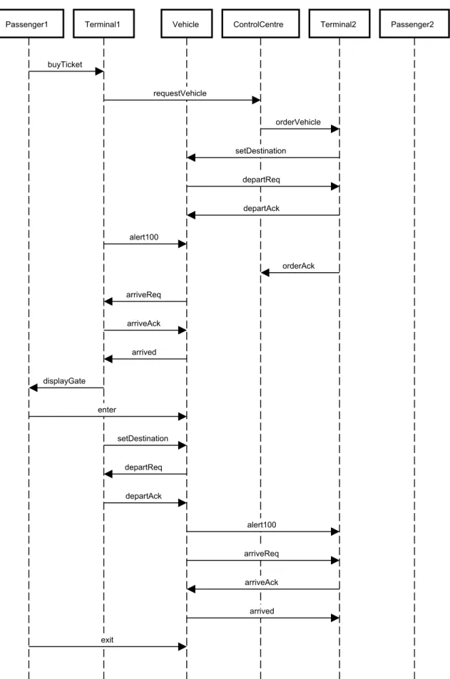
5.2.1 Case Study 1: A Passenger Transportation System . . . 43
System Description . . . 43
Analysis . . . 43
Summary . . . 48
5.2.2 Case Study 2: Boiler System . . . 49
System Description . . . 49
Analysis . . . 49
Summary . . . 51
5.2.3 Case Study 3: Cruise Control System . . . 51
System Description . . . 51
Analysis . . . 52
Summary . . . 59
5.2.4 Case Study 4: Distributed Smart Camera System . . . 60
System Description . . . 60
Analysis . . . 60
Summary . . . 66
5.2.5 Case Study 5: eB2B System . . . 67
System Description . . . 67
Analysis . . . 67
Summary . . . 71
5.2.6 Case Study 6: Global System for Mobile Mobility Management System 73 System Description . . . 73
Analysis . . . 75
Summary . . . 80
5.2.7 Case Study 7: Semantic Search Multi-Agent System . . . 80
System Description . . . 80
Analysis . . . 81
Summary . . . 84
5.3 Discussion . . . 86
5.3.1 Threats to Validity . . . 89
6 Conclusion & Future Work 91
Appendix 96
A Systems Scenarios 97
A.1 A Passenger Transportation System (APTS) . . . 97
A.2 Boiler . . . 100
A.3 Cruise Control (Cruiser) . . . 103
A.4 Distributed Smart Camera (SmartCam) . . . 107
A.5 eB2B . . . 117
A.6 Global System for Mobile Mobility Management (GSM) . . . 123
List of Figures
2.1 bMSCs representing the Boiler’s scenarios. . . 6
2.2 hMSC of the Boiler system specification. . . 8
2.3 Each Boiler component’s LTS representing the messages exchanged. . . 9
2.4 Resulting LTS of the parallel composition of the LTSs in ?? 2.3. . . 10
2.5 Each Boiler component’s FSP. . . 11
2.6 An implied scenario from the boiler system. . . 12
2.7 Example of a clustering technique, taken from [1]. . . 13
2.8 Plot of example datapoints. . . 15
2.9 Dendrogram showing the order of grouping. . . 16
2.10 Example results for the Smith-Waterman algorithm. . . 18
4.1 Steps of the proposed methodology. . . 25
4.2 Boiler model opened in the LTSA-MSC tool. . . 35
4.3 Dialogs of start and finish of IS collection process. . . 35
4.4 The collected ISs for the Boiler example. . . 36
4.5 Example of a common behavior detection. . . 36
4.6 Second CB for the Boiler system. . . 36
4.7 Smith-Waterman applied to Boiler’s common behaviors. . . 37
4.8 Dendrogram for the Boiler example. . . 37
4.9 LTS of the constraint used to treat Boiler’s first common behavior. . . 38
4.10 LTS of the Boiler constrained architecture model. . . 39
4.11 Traces reached in the Boiler original model. . . 40
4.12 Traces reached in the Boiler constrained model. . . 41
5.1 hMSC for APTS specification. . . 43
5.2 ISs collected for APTS. . . 44
5.3 Traces reached in APTS original model. . . 44
5.4 Dendrogram for APTS. . . 45
5.5 First constraint for APTS. . . 45
5.7 Second constraint for APTS. . . 46
5.8 Traces reached in APTS second constrained model. . . 47
5.9 Third constraint for APTS. . . 47
5.10 Traces reached in APTS third constrained model. . . 48
5.11 Traces reached in Boiler original model. . . 50
5.12 Traces reached in Boiler first constrained model. . . 50
5.13 Second constraint for Boiler. . . 51
5.14 Traces reached in Boiler second constrained model. . . 51
5.15 hMSC for Cruiser specification. . . 52
5.16 CBs detected for Cruiser. . . 53
5.17 Traces reached in Cruiser original model. . . 54
5.18 Dendrogram for Cruiser. . . 54
5.19 First constraint for Cruiser. . . 55
5.20 Traces reached in Cruiser first constrained model. . . 56
5.21 Second constraint for Cruiser. . . 57
5.22 Traces reached in Cruiser second constrained model. . . 58
5.23 Third constraint for Cruiser. . . 58
5.24 Traces reached in Cruiser third constrained model. . . 59
5.25 hMSC for SmartCam specification. . . 60
5.26 ISs collected for SmartCam. . . 61
5.27 Traces reached in the SmartCam original model. . . 62
5.28 Dendrogram for SmartCam. . . 62
5.29 First constraint for SmartCam. . . 63
5.30 Traces reached in SmartCam first constrained model. . . 64
5.31 Second constraint for SmartCam. . . 64
5.32 Traces reached in SmartCam second constrained model. . . 65
5.33 Third constraint for SmartCam. . . 66
5.34 Traces reached in SmartCam third constrained model. . . 66
5.35 hMSC for eB2B specification. . . 68
5.36 Traces reached in the eB2B original model. . . 69
5.37 CBs detected for eB2B. . . 70
5.38 Dendrogram for eB2B. . . 71
5.39 Constraint for eB2B. . . 71
5.40 Traces reached in eB2B constrained model. . . 72
5.41 GSM hMSC. . . 74
5.42 CBs detected for GSM. . . 76
5.44 Dendrogram for GSM. . . 77
5.45 LTS of GSM’s constraint. . . 79
5.46 Traces reached in GSM constrained model. . . 79
5.47 hMSC of S.S. MAS. . . 80
5.48 Collected ISs for S.S. MAS. . . 81
5.49 Traces reached in S.S. MAS original model. . . 82
5.50 Dendrogram for S.S. MAS. . . 82
5.51 Initial constraint for S.S. MAS. . . 83
5.52 Traces reached in S.S. MAS first constrained model. . . 83
5.53 Altered constraint for S.S. MAS. . . 84
5.54 Traces reached in S.S. MAS second constrained model. . . 85
A.1 APTS’s hMSC. . . 97
A.2 bMSC for APTS’s VehicleAtTerminal scenario. . . 98
A.3 bMSC for APTS’s VehicleNotAtTerminal scenario. . . 99
A.4 Boiler’s hMSC. . . 100
A.5 bMSC for Boiler’s Analysis scenario. . . 101
A.6 bMSC for Boiler’s Initialise scenario. . . 101
A.7 bMSC for Boiler’s Register scenario. . . 101
A.8 bMSC for Boiler’s Terminate scenario. . . 102
A.9 Cruiser’s hMSC. . . 103
A.10 bMSC for Cruiser’s Scen1. . . 104
A.11 bMSC for Cruiser’s Scen2. . . 105
A.12 bMSC for Cruiser’s Scen3. . . 105
A.13 bMSC for Cruiser’s Scen4. . . 106
A.14 SmartCam’s hMSC. . . 107
A.15 bMSC for SmartCam’s Scenario1. . . 108
A.16 Trajectory depicted in SmartCam’s Scenario1, taken from [2]. . . 109
A.17 bMSC for SmartCam’s Scenario2. . . 110
A.18 Trajectory depicted in SmartCam’s Scenario2, taken from [2]. . . 111
A.19 bMSC for SmartCam’s Scenario3. . . 111
A.20 Trajectory depicted in SmartCam’s Scenario3, taken from [2]. . . 112
A.21 bMSC for SmartCam’s Scenario4. . . 113
A.22 Trajectory depicted in SmartCam’s Scenario4, taken from [2]. . . 114
A.23 bMSC for SmartCam’s Scenario5. . . 115
A.24 Trajectory depicted in SmartCam’s Scenario5, taken from [2]. . . 116
A.25 eB2B’s hMSC. . . 117
A.27 bMSC for eB2B’s Criteria scenario. . . 118
A.28 bMSC for eB2B’s DetailsView scenario. . . 119
A.29 bMSC for eB2B’s FailedLogin scenario. . . 119
A.30 bMSC for eB2B’s HeaderView scenario. . . 120
A.31 bMSC for eB2B’s ItemDetails scenario. . . 120
A.32 bMSC for eB2B’s Login scenario. . . 121
A.33 bMSC for eB2B’s Logout scenario. . . 121
A.34 bMSC for eB2B’s ShutDown scenario. . . 122
A.35 bMSC for eB2B’s StartUp scenario. . . 122
A.36 GSM’s hMSC. . . 123
A.37 bMSC for GSM’s Accept1, Accept2, Accept3 scenarios. . . 124
A.38 bMSC for GSM’s Authenticate1, Authenticate2, and Authenticate3 sce-narios. . . 124
A.39 bMSC for GSM’s CallSetupReq scenario. . . 125
A.40 bMSC for GSM’s ConnReq scenario. . . 125
A.41 bMSC for GSM’s Encrypt1, Encrypt2, and Encrypt3 scenarios. . . 126
A.42 bMSC for GSM’s Identify1, Identify2, and Identify3 scenarios. . . 126
A.43 bMSC for GSM’s LocationUpd scenario. . . 127
A.44 bMSC for GSM’s LocUpdReq scenario. . . 127
A.45 bMSC for GSM’s MobileOrCR scenario. . . 128
A.46 bMSC for GSM’s MobileOrCS scenario. . . 129
A.47 bMSC for GSM’s MobileTrCR scenario. . . 130
A.48 bMSC for GSM’s MobileTrCS scenario. . . 131
A.49 bMSC for GSM’s PagingResp scenario. . . 132
A.50 bMSC for GSM’s Reject1, Reject2, and Reject3 scenarios. . . 132
A.51 S.S. MAS’s hMSC. . . 133
A.52 bMSC for S.S. MAS’s MSC1 . . . 134
List of Tables
2.1 Coordinates of example datapoints in x and y axis. . . 15
2.2 Euclidean distances between example datapoints. . . 15
2.3 Euclidean distances after first recursion. . . 16
3.1 Related work comparison . . . 23
5.1 Time spent and # of CBs per ISs for Boiler . . . 49
5.2 Time spent and # of CBs per ISs for Cruiser . . . 52
5.3 Time spent and # of CBs per ISs for eB2B . . . 67
5.4 Time spent and # of CBs per ISs for GSM . . . 75
5.5 Summary of results across all systems studied . . . 86
5.6 Number of CBs detected per number of ISs collected . . . 87
5.7 Time (h:m:s) to collect n implied scenarios . . . 87
Chapter 1
Introduction
1.1 Context
A useful way to model distributed systems’ specifications is to use scenarios. A scenario depicts how different components interact to achieve a common goal. Message Sequence Charts [3] and UML sequence diagrams [4] are two commonly used methods to design and display these scenarios. Both of these techniques use the idea of components that send each other messages, that is, two different components that need to work together to achieve a goal can interact synchronously or asynchronously with each other through message passing.
Although widely used, a scenario specification can describe only partial behaviors of a system, while its implementation has full behaviors [5]. Such limitations can lead to a common fault in scenario specifications, which are implied scenarios. Implied scenarios are unexpected behaviors that can emerge at runtime due to components’ interactions that are implied in the specification [5]. That is, different components believe they are behaving correctly on its own, but the composition of all their actions together is not included in the original specification. More formally, “implied scenarios indicate gaps in a scenario-based specification that are the result of specifying the behavior of a system from a global perspective yet expecting the behavior to be provided in a local component-wise fashion by independent entities with a local view of the system” [6].
Even though implied scenarios can lead to unexpected behaviors, they are not al-ways unacceptable behaviors [7]. An implied scenario can be a positive scenario that was overlooked in the original specification or be indeed an unacceptable behavior. For the for-mer, it can be simply included in the specification, while the latter has to be constrained. Therefore, implied scenarios should be detected and validated with stakeholders [8] to de-fine how to deal with them. If left untreated these scenarios can cause damage if they lead to unwanted behaviors [9]. Particularly, implied scenarios can affect the reliability [10,11]
and security [12] of a system. Thus, it is desirable to deal with these implied scenarios before the system is up and running to prevent unwanted behavior. However, the pro-cess of detecting implied scenarios has been proved to be undecidable by Chakraborty et al. [13], meaning that there is no guarantee that the detection of all implied scenarios of a given system will ever stop in polynomial time.
1.2 Problem
Several approaches to detect implied scenarios have been devised (e.g., [5–7,14–16]). Most of them, however, do not go further on the process of dealing with implied scenarios, that is, they stop their methodologies after detecting implied scenarios. In other words, they neither suggest a solution nor try to find the root of the underlying cause. By doing so, it can lead the user to spend a lot of time analyzing a large number of implied scenarios. Some exceptions, such as Uchitel et al. [6], Song et al. [5], and Moshirpour et al. [16], show the cause to the user and suggest solutions for the problem to be fixed. However, these approaches can still output a large number of implied scenarios, which can be cumbersome to the user. Since these approaches do not further investigate the correlation between the implied scenarios, they could misguide the user on how to deal with such implied scenarios at large.
1.3 Research Questions and Contributions
Based on these problems, three research questions are raised, which motivates the contri-butions of the dissertation.
Research Question 1 Can we provide a heuristic to restrict the problem space
of implied scenarios analysis?
To answer this first question, a new methodology is proposed to fill in the literature gap, which is achieved by finding common behaviors among implied scenarios that lead the system to unexpected behavior. The process of detecting the common behaviors consists of two major steps: (i) collect multiple implied scenarios and (ii) detect common behaviors among them. For the first step, we extend the approach by Uchitel et al. [6], where we automated the process of collecting implied scenarios, that is, instead of detecting a single IS, our approach iteratively collects multiple distinct ISs without the need of user interaction. From these collected implied scenarios, their underlying core common behaviors are extracted. By these means, we restrict the problem space of the
undecidability of implied scenario detection by treating the implied scenarios as a group, instead of individually. Therefore, we answer Research Question 1, as we successfully restricted the problem space that the user needs to analyze.
Research Question 2 Can we semantically group the common behaviors in a sound manner?
Following, we group the common behaviors that were detected. This is achieved by hierarchically clustering them, and in order to calculate the distance among the common behaviors we use one of the several string matching algorithms that exist in the litera-ture: the Smith-Waterman algorithm [17], widely used in bioinformatics research. This algorithm is used to identify the best local alignment between genetic sequences, that is, it tries to find which parts of the two DNA sequences have the most in common. Thus, it can be successfully used to find the underlying sequences that are shared among common behaviors. By using this algorithm, we were able to find semantically defined groups of common behaviors, which helps the user analysis of the system. Therefore, by these means we are able to semantically group the common behaviors, answering Research Question 2. Furthermore, we compare the clustering results with the ones obtained using the Levenshtein distance [18], in order to support the choice for the Smith-Waterman algorithm.
Research Question 3 Is it possible to state there is an underlying cause among
the groups of common behaviors?
Next, a manual analysis of the groups is required. By doing so, it is possible to identify underlying causes among common behaviors by looking at the alignments obtained with the Smith-Waterman algorithm. Therefore, it is possible to define groups of common behaviors that share the same underlying cause. We call such groups families of common
behaviors. If the underlying cause of a family is undesirable, that is, it deviates from the
wanted behavior of the system, it is a fault. Thus, if it is not treated, it may lead to system failures. As a proof of concept, all underlying causes were considered to be faults. After that, each family of common behaviors was dealt with in a single fix. In other words, we were able to resolve all common behaviors in the family, by constraining their underlying cause and not each one individually. By these means, we are able to success-fully identify the underlying cause among a family of common behaviors. As a result, we contribute to answering both Research Question 3 and a research question previously raised by Uchitel et al. [8]: “should the entire implied scenario be constrained or is the
unaccepted situation due to a specific subsequence of actions that appear in the implied scenario?” In fact, our results explicitly show that it is possible to prevent unaccepted
situations by constraining specific underlying causes of common behaviors, which we can detect by characterizing families.
Finally, in order to evaluate the proposed methodology, we performed seven case stud-ies with system specifications reported in the literature. Throughout these case studstud-ies, we collected a total of 1798 implied scenarios, which demanded nearly 37 hours of exe-cution. From these implied scenarios, our methodology was able to come up with only 14 families of common behaviors, where each family required a single constraint and each system specification required at most three constraints to prevent all collected implied scenarios. Additionally, our methodology shows that the same 14 families could have been found with 424 collected implied scenarios instead of the original 1798. This would reduce the timespan of the detection process from nearly 37 hours to under 24 minutes. Thus, the main contribution of this dissertation is the methodology which facilitates the analysis of multiple implied scenarios.
1.4 Outline
The rest of this dissertation is structured as follows: Chapter 2 introduces and details technical concepts used in the methodology; Chapter 3 discusses the related work in the literature; Chapter 4 explains the proposed methodology in further details and uses an example system to illustrate the approach; Chapter 5 shows and discusses the results obtained through seven case studies; finally, Chapter 6 summarizes the contributions from this dissertation and introduces some ideas for future work.
Chapter 2
Background
In this chapter, definitions and technical concepts that are used throughout this disserta-tion will be laid out and explained with examples, where applicable.
2.1 Scenarios
“Scenarios describe how system components, the environment and users work concurrently and interact in order to provide system level functionality” [6]. Simply put, a scenario is a description of a system’s action. It describes what the user expects from the system when interacting with it. We can model entire systems based solely on scenarios that it needs to execute, this is called a positive scenario-based model by Uchitel et al. [6].
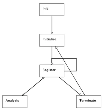
The Boiler System [6] will be used as a running example. The Boiler System is a system that controls the temperature inside a boiler, according to the measured pressure by its sensor. It has the following components:
Actuator variates the temperature inside the boiler;
Control tells the actuator to act according to the last pressure measured; Database stores the measured pressures;
Sensor measures the pressure inside the boiler.
This system performs four scenarios, and these are all accomplished by interactions between the components. Below these scenarios are shown and the interactions between the system’s components are described:
Initialise
Sensor Database Control Actuator
on
Register
Sensor Database Control Actuator
pressure
Analysis
Sensor Database Control Actuator
query data
command
Terminate
Sensor Database Control Actuator
off
Figure 2.1: bMSCs representing the Boiler’s scenarios.
Register : Sensor sends Database the current pressure so it is stored and can be queried
later on;
Analysis : Control queries Database for the latest pressure and tells Actuator to alter
the boiler’s temperature accordingly.
By implementing these four scenarios, we have a system that was modeled on a scenario-based way.
2.1.1 Message Sequence Chart
A message sequence chart (MSC) is a simple and intuitive graphical representation of a scenario [3]. It explicitly shows the interactions between components, by showing each one of those as a message sent from one component to another. We can use MSCs to show the Boiler System’s scenarios described above as in Figure 2.1. As it can be seen, it is a convenient way to exemplify the interactions that happen for a scenario to be achieved.
The MSCs shown in Figure 2.1 are said to be basic message sequence charts (bMSCs), which describe a finite interaction between a set of components [6]. In the Initialize sce-nario for instance, the Control instance is sending the message on to the Sensor instance. A bMSC does not necessarily convey an order to the messages. However, in our case, there is only one bMSC with more than one message. Therefore, the other ones have only one possible order of execution, which is sending their only message.
For the Analyse bMSC however, there are three messages that could lead to more possible orders of execution. In this case, it is important to note that an instance of a bMSC has to follow the order on which the messages are sent or received. For instance, the Database instance can only send the data message after the query message is received. Hence, this scenario only has one possible order as well. Formally, Definition 1 shows how bMSCs are defined by Uchitel et al. [6].
Definition 1 [Basic Message Sequence Chart] A basic message sequence chart
(bMSC) is a structure b = (E, L, I, M, instance, label, order) where: E is a countable set of events that can be partitioned into a set of send and receive events that we denote send(E) and receive(E). L is a set of message labels. We use –(b) to denote L.
I is a set of instance names. M : send(E) æ receive(E) is a bijection that pairs send
and receive events. We refer to the pairs in M as messages. The function instance:
E æ I maps every event to the instance on which the event occurs. Given i œ I, we denote {e œ E|instance(e) = i} as i(E). The function label: E æ L maps events to labels. We require for all (e, eÕ) œ M that label(e) = label(eÕ), and if (v, vÕ) œ M and
label(e) = label(v), then instance(e) = instance(v) and instance(eÕ) = instance(vÕ).
order is a set of total orders Æi™ i(E) ◊ i(E) with i œ I and Æi corresponding to
the top-down ordering of events on instance i.
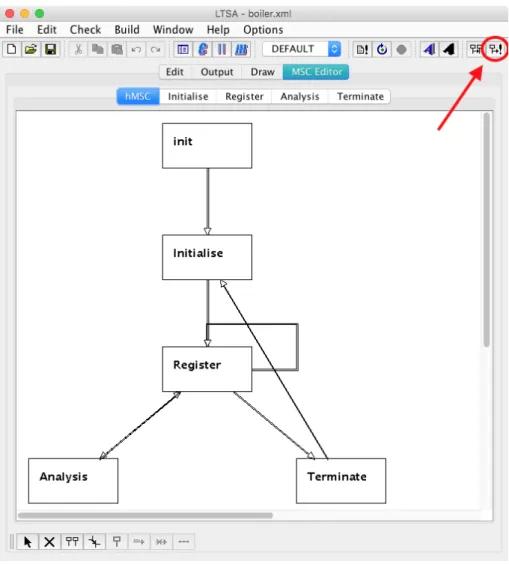
An extension of bMSCs are high-level message sequence charts (hMSCs), which pro-vides the means for composing bMSCs [6]. These can be used to show the possible paths of execution of a system, that is, the possible continuations after each bMSC, in a way that it is visually and easily understood. As an example, in Figure 2.2 the hMSC for the
Boiler System is shown. It is possible to observe that the scenarios are ordered in a way
that the system delivers correct service. The formal definition of hMSCs by Uchitel et al. [6] is presented in Definition 2.
Definition 2 [High-Level Message Sequence Charts] A high-level message sequence
chart (hMSC) is a graph of the form (N, E, s0) where N is a set of nodes, E ™ (N◊N)
is a set of edges, and s0 œ N is the initial node. We say that n is adjacent to nÕ if
(n, nÕ) œ E. A (possibly infinite) sequence of nodes w = n0, n1, ...is a path if n0 = s0,
and ni is adjacent to ni+1 for 0 Æ i < |w|. We say a path is maximal if it is not a
proper prefix of any other path.
Finally, the hMSC depicted in Figure 2.2 is a special kind of hMSC, which is called a Positive Specification (PSpec). Simply put, a PSpec contains an hMSC, a set of bMSCc, and a bijective function that maps one node from the hMSC to a single bMSC. The formal
Figure 2.2: hMSC of the Boiler system specification. definition by Uchitel et al. [6] is presented in Definition 3.
Definition 3 [Positive Message Sequence Chart Specification] A positive message
sequence chart (MSC) specification is a structure P Spec = (B, H, f) where B is a set of bMSCs, H = (N, A, s0) is a hMSC, and f : N æ B is a bijective function that
maps hMSC nodes to bMSCs. We use –(P Spec) = {l|÷b œ B.l œ –(b)} to denote the alphabet of the specification.
2.1.2 Labeled Transition System
A labeled transition system (LTS) is a finite state machine that has an intuitive easily grasped semantics and a simple representation [19]. They can be used to represent the expected order of messages exchanged by each component of a distributed system.
An LTS is a directed graph, with nodes and edges, where each node represents a state of the system, and each edge a transition from one state to another. Edges are labeled with the message(s) that are exchanged for that transition to happen. Finally, there is a unique node that represents the initial state of the system (state 0), which will be denoted in red. More formally, Definition 4 shows the definition of LTSs by Uchitel et al. [6].
Definition 4 [Labeled Transition Systems] Let States be the universal set of states
where state fi is the error state. Let Labels be the universal set of message labels and Labels· = Labels fi · where · denotes an internal component action that is
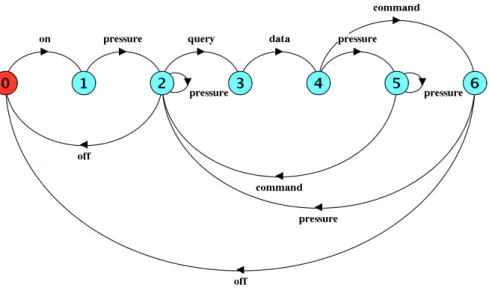
Figure 2.3: Each Boiler component’s LTS representing the messages exchanged. unobservable to other components. An LTS P is a structure (S, L, —, q) where S ™
States is a finite set of states, L = –(P ) fi ·, –(P) ™ Labels is a set of labels that
denotes the communicating alphabet of P , — ™ (S\{fi} ◊ L ◊ S) defines the labeled transitions between states, and q œ S is the initial state. We use s l
æ sÕ to denote
(s, l, sÕ) œ — . In addition,we say that an LTS P is deterministic if s æ s1 andl
s æ s2 implies s1 = s2.l
Figure 2.3 shows the LTS for each component of the Boiler system. For instance, the LTS for the Sensor shows that this component, the first message to be exchanged must be
on, then pressure, and so on. Note that each LTS contains only the messages exchanged
by that component (e.g., the LTS for the Actuator has only one state and one transition, because that component only exchanges one message throughout all scenarios).
Finally, it is possible to combine different LTSs by doing a parallel composition of them. The resulting LTS represents the expected order of messages in the entire system. Figure 2.4 shows the resulting LTS of the parallel composition of the LTSs in Figure 2.3. Formally, the definition of parallel composition by Uchitel et al. [6] is presented in Def-inition 5. The only exceptions to the rules presented are that state fi is used instead of states (x, fi) and (fi, x) for all x œ States.
Definition 5 [Parallel Composition of LTS] Let P1 and P2 be LTSs where Pi =
(Si, Li,—i, qi). Their parallel composition is denoted P1||P2and is an LTS (S, L, —, q)
where S = S1◊ S2fi {fi, ‘}, L = L1fi L2, q= (q1, q2), and — is the smallest relation in
(S\{fi})◊L◊S that satisfies the following rules where x a
æi ydenotes (x, a, y) œ —i:
s æa1 t
(s, sÕ)æ (t, sa Õ)(a /œ –(L2)),
sæa2 t
Figure 2.4: Resulting LTS of the parallel composition of the LTSs in Figure 2.3.
sæa1 tsÕ æa2 tÕ
(s, sÕ)æ (t, ta Õ)(a /œ (–(L1) fl –(L2))\{·}).
Finite State Process Notation
The Finite State Process (FSP) is a notation used to specify the behavior of concurrent systems to the Labelled Transition System Analyzer (LTSA) tool1 [?]. A FSP specification
generates LTSs, such as the ones in Figures 2.3 and 2.4. FSP specifications contain two sorts of definitions: primitive processes (e.g., individual components) and composite processes (e.g., parallel compositions).
For primitive processes, only the notion of states, action prefix, and choice will be used. A state represents a state in an LTS, and is named Qi (i = 0,1,2...). It is denoted by Qi = (a), where a is either an action prefix or a choice and represents the existing transitions that leave this state. The action prefix represents a transition in an LTS, and is denoted by a -> b, where a is a message and b is either a message or a state. It indicates that after a is exchanged, the LTS will either change to state b or wait for message b to be exchanged. Finally, choice is denoted by a | b, where a is an action prefix and b is either an action prefix or a choice . It indicates that more than one transition exist leaving that state. Figure 2.5 shows the FSPs that generates the corresponding LTSs in Figure 2.3.
Finally, the only composite process used in this dissertation will be parallel composi-tion. It is analogous to the parallel composition of LTSs, and it is detonated by (a||b), where a is a primitive process, and b is either a primitive process or a parallel
Control = Q0, Q0 = (on -> Q1), Q1 = (off -> Q0 |query -> Q2), Q2 = (data -> Q3), Q3 = (command -> Q1). Database = Q0, Q0 = (pressure -> Q1), Q1 = (pressure -> Q1 |query -> Q2), Q2 = (data -> Q0). Actuator = Q0, Q0 = (command -> Q0). Sensor = Q0, Q0 = (on -> Q1), Q1 = (pressure -> Q2), Q2 = (off -> Q0 |pressure -> Q2).
Figure 2.5: Each Boiler component’s FSP.
position. The FSP corresponding to the parallel composition of the Boiler components (Boiler = (Control||Database||Actuator||Sensor)) generates the LTS in Figure 2.4.
2.1.3 Implied Scenarios
An implied scenario (IS) is a scenario that was not included in the system’s specifica-tion, but it occurs in every implementation of the specification [20]. It is a result from implementing actions that are global to the system, in a local level to the components that executes them. Because of this implementation, a component might not have enough information locally to decide whether or not the action should be prevented, therefore it is always performed.
An implied scenario can be classified as positive or negative [6]. A positive implied scenario is one that although it was not included in the system specification and its behavior was not expected, it has a desired behavior. Thus, a positive IS represents an unexpected but acceptable behavior. In this case, the system’s specification is usually extended with this new scenario. On the other hand, a negative implied scenario is a scenario that was not expected and its observed behavior is harmful to the system’s execution. That is, the system is not performing the correct service, or in other words, performing a failure. Thus, a negative IS represents an unexpected unacceptable behavior. However, in the present work, this distinction will be disregarded, and therefore all ISs will be treated as a failure for simplicity since the characterization of a positive IS requires domain-expert knowledge. Although this can introduce an unnecessary cost to the system, as we might add constraints to the system in order to restrict behaviors that could instead be included, this analysis is not in the scope of this work, as our goal is to demonstrate the possibility of resolving various ISs at once.
Because of the nature of concurrent systems, implied scenarios may not happen in every system run, as messages are not synchronized and traces of execution (order of the
Figure 2.6: An implied scenario from the boiler system.
messages on the MSC) could be different, even though the same course of action is sought. As an example, in Figure 2.6 an implied scenario in the Boiler System is presented. The unexpected part, that is, the cause of the implied scenario, is that Control tries to execute the Analysis scenario before a pressure from the current system run is registered. Therefore, it will tell the Actuator to variate the temperature according to a pressure that does not represent the system’s current state.
Finally, to formally define what is an implied scenario, we use Definitions 6 to 10 from Uchitel et al. [6]. These definitions show that an implied scenario is a system execution that is not modeled in P Spec but arises in every architecture model of P Spec. That is, it is an unexpected execution that happens in all implementations of P Spec.
Definition 6 [Execution] Let P = (S, L, —, q) be a LTS. An execution of P is a
sequence w = q0l0q1l1...of states qi and labels li œ L such that q0 = q and qi li
æ qi+1
for all 0 Æ i < |w/2|. An execution is maximal if it cannot be extended to still be an execution of the LTS. We also define ex(P ) = {w | w is an execution of P }.
Definition 7 [Projection] Let w be a word w0w1w2w3... and A an alphabet. The
projection of w onto A, which we denote w|A, is the result of eliminating from the word w all elements wi in A.
Definition 8 [Trace and Maximal Trace] Let P be a LTS. A word w over the
alphabet –(P ) is a (maximal) trace of P if there is an (maximal) execution e œ ex(P) such that w = e|–(P). We use tr(e) to denote the projection of an execution on the
alphabet of a LTS. We also define tr(P ) = {w | w is a trace of P } and L(P ) = {w|w is a maximal trace of P }.
Definition 9 [Architecture Models] Let P Spec = (B, H, f) be a positive MSC
specification with instances I, and let Ai with i œ I be LTSs. We say that an LTS
A is an architecture model of P Spec only if A = (A1|| ... ||An), –(Ai) = –(i), and
L(P Spec) ™ L(A).
Definition 10 [Implied Scenarios] Given a positive MSC specification P Spec, a
trace w /œ L(PSpec) is an implied scenario of PSpec if for all trace y and for all architecture model A of P spec, w.y œ L(A) implies w.y /œ L(PSpec).
2.2 Clustering
Another important background required in this work is the one regarding the notion of clustering. Clustering is a data-mining technique used to group datapoints in a dataset. In other words, it is a method to group elements in an unsupervised way. After obtaining the separate groups, the user still has to analyze the results and figure out why those elements were clustered together. A simple definition of the clustering process is given in Matteucci [1]: "the process of organizing objects into groups whose members are similar in some way".
A good clustering result is such that the cluster elements are very similar to each other, and very dissimilar to other clusters’ elements. This way a good separation between clusters is observed and the elements within a cluster are clearly similar.
In Figure 2.7 a simple clustering process is shown, where on the left side of the image the elements are all separate, and on the right side, after clustering, four clusters can be clearly seen.
2.2.1 Hierarchical Clustering
As defined by Ward [21], Hierarchical Grouping – later called Hierarchical Clustering by Johnson [22] – is “a procedure for forming hierarchical groups of mutually exclusive
subsets, each of which has members that are maximally similar with respect to specified characteristic”. There are two types of hierarchical clustering [23]: agglomerative and
divisive. The former starts with N clusters, containing 1 element each, and groups clusters one by one until there is only one cluster. The latter starts with 1 cluster, containing all N elements, and splits the existing clusters until there are N clusters, containing 1 element each.
The agglomerative hierarchical clustering is a method where members of a dataset (datapoints) are grouped hierarchically, with the most similar datapoints (or groups of datapoints) being merged before the less similar ones. This similarity is often measured by a distance metric, which means that the lower the score between two datapoints, the more similar they are.
This process is recursive [22] and consists of four steps: (i) calculate the similarity (or distance) between all members of the current dataset; (ii) find the most similar pair between those members; (iii) replace those two members with a new one, which merely is the two grouped together; (iv) go to (i) if there is more than one member in the current dataset. In the end, there will be a single member of the dataset, which is a group containing all individual datapoints that made up the original dataset. The interesting result, however, is being able to see the step-by-step grouping of members, which facilitates the detection of subgroups in the dataset.
The divisive hierarchical clustering is a method where all members start in the same cluster, and then are split into smaller clusters until each member is in a cluster by itself. One possible way to achieve this is by using the DIvisive ANAlysis Clustering (DIANA) [24], where the largest cluster is broken down in every step. First, the element
e that is most dissimilar to the other ones is selected and removed from that cluster;
Then, the remaining elements that are more similar to e than to the other remaining ones are also moved to that new cluster. This process is repeated until all elements have been separated.
However, because the initial merges of small-size clusters in the agglomerative ap-proach correspond to high degrees of similarity, its results are more understandable than the ones obtained by the divisive approach [25]. Therefore, as the clustering results will serve as a reference to the user in our methodology, it is essential that its results be un-derstandable and help the user to analyze the elements grouped. Thus, the agglomerative approach is used and from here on hierarchical clustering will be used to refer to the agglomerative approach.
Coordinates of example datapoints in x and y axis.
A B C D E
x 1 0 2 4.5 6
y 2 1 1 6 6
Figure 2.8: Plot of example datapoints.
As an example, let us consider five datapoints in a 2-dimensional plot. These points are represented in Figure 2.8 and their coordinates are shown in Table 2.1. To apply the algorithm, it is required to have the similarity between the elements. Table 2.2 shows the Euclidean distance between these points. With this information, the first pair to be grouped could be either A and B or A and C, as they have the smallest distance between them with 1.41. Without loss of generality, A and B will be the first elements to be grouped.
The question now is how to calculate the similarity between a group of datapoints ({A, B}) and other datapoints. In fact, there are multiple ways to achieve this, such as: (i) complete linkage clustering [26], which calculates the distance between a group of elements E and another element eÕ as the maximum possible distance of e œ E and eÕ;
(ii) single linkage clustering [26], where the distance between a group of elements E and another element eÕ is the minimum possible distance of e œ E and eÕ; and (iii) Ward’s
Euclidean distances between example datapoints.
A B C D E A 0 B 1.41 0 C 1.41 2.0 0 D 5.32 6.73 5.59 0 E 6.40 7.81 6.40 1.5 0
Euclidean distances after first recursion. {A ,B} C D E {A, B} 0 C 2.0 0 D 6.73 5.59 0 E 7.81 6.40 1.50 0
Figure 2.9: Dendrogram showing the order of grouping.
method [21], which calculates the increase in variance if two clusters were merged. The
method used to exemplify will be the “complete linkage clustering” [26].
By using the complete linkage method, the highest distance between a member of the group and another member is kept, that is, the distance between {A, B} and C will be 2.0, as that is the maximum value between 1.41 (dist(A, C)) and 2.0 (dist(B, C)). This way, the distances after the first recursion are shown in Table 2.3. The process is then repeated with these new distances, and the next members to be grouped will be D and E, as these datapoints have a distance of 1.50, which is the lowest distance on this current dataset.
The final result of the whole process is shown in Figure 2.9. This kind of graph is called a dendrogram, which provides a useful visual way to analyze hierarchical clusters, allowing a different analysis of the dataset. For instance, on this example, it is clear that two groups are formed, as A, B, and C are much closer to one another than they are to D and E. Similarly, D and E are more similar to each other than to the other 3 points.
2.3 Smith-Waterman Algorithm
The Smith-Waterman algorithm (SW), first introduced by Smith & Waterman in [17], proposes to “find a pair of segments, one from each of two long sequences, such that there
is no other pair of segments with greater similarity” [17]. In other words, SW tries to find
the best local alignment between two sequences, local in the sense that this alignment can be shorter than the sequences, that is, it might find only a small part of the sequences where they are most similar. It is widely used in bioinformatics research to calculate the similarity between genetic sequences.
The algorithm can be broken down into two steps: (i) calculate the scoring matrix; and (ii) traceback the best alignment from the highest value in the matrix.
Therefore, firstly it is needed to calculate the scoring matrix (SM). The SM is a (n+1) by (m + 1) matrix, where n and m are the lengths of the sequences to be compared. The first column and row are filled with zeros, while the rest of the matrix is filled according to the recurrence equation shown in Equation (2.1), where, A and B are the sequences being compared, and s(Ai, Bj) checks if Ai and Bj are the same element. If they are it returns
M AT CH, if not it returns MISMAT CH. Lastly, GAP , MAT CH, and MISMAT CH
are defined by the user.
SMi,j = max Y _ _ _ _ _ _ _ _ ] _ _ _ _ _ _ _ _ [ SMi≠1,j+ GAP SMi,j≠1+ GAP SMi≠1,j≠1+ s(Ai, Bj) 0 (2.1)
Simply put, each cell SMi,j is calculated with basis on previously calculated values
– SMi≠1,j, SMi≠1,j≠1, and SMi,j≠1 – but only one of these values is used at most. If
the upper-left diagonal value (SMi≠1,j≠1) is used, then it indicates that both sequences
are reading their elements (i.e., Ai, Bj); thus, it is considered whether Ai = Bj, and a
value (MAT CH or MISMAT CH) is used to calculate SMi,j accordingly. However, if
the upper value (SMi≠1,j) is used, only A is reading its element, as it goes from Ai≠1 to
Ai while Bj is constant. Analogously, for the left value (SMi,j≠1) Ai is constant and Bj≠1
changes to Bj. For these two last cases, a penalty (GAP ) for not considering elements
from both sequences is used to calculate SMi,j.
After the whole SM has been populated, we can find the best local alignment. This is achieved by doing a traceback from the highest value found in the SM, which is the score of the best alignment. First, we have to find the highest value in SM, which represents the end of the best alignment. Let us assume (k, l) is such position. Starting from this
G C T C G 0 0 0 0 0 0 A 0 0 0 0 0 0 C 0 0 3 1 3 1 T 0 0 1 G 0 3 1 A 0 1 0 2
(a) single cell calculation
G C T C G 0 0 0 0 0 0 A 0 0 0 0 0 0 C 0 0 3 1 3 1 T 0 0 1 6 4 2 G 0 3 1 4 3 7 A 0 1 0 2 1 5 1 (b) scoring matrix Best Alignment: C T — G C T C G Score: 7
(c) alignment and score
Figure 2.10: Example results for the Smith-Waterman algorithm.
and SMk,l≠1. The cell with the highest value among those is a part of the alignment,
and thus it is included in the traceback. This procedure is repeated with each new cell included until the next new cell has a value of zero. Finally, the alignment is the reversed sequence of cells included (as the first cell represents the end of the alignment), where movements in the horizontal consider only one sequence, vertical movements consider the other sequence, and diagonal movements consider both sequences.
As an example, let A = ACTGA, B = GCTCG, MAT CH = 3, MISMAT CH = -3, and GAP = -2. Figure 2.10a shows the calculation for a single cell, in this case, SM4,4.
The arrows represent which neighbors cells that can help to fill this one. From the left (SM4,3) and above (SM3,4) cells, the GAP penalty would apply, so both send a value of
1+(-2). For the diagonal cell (SM3,3), we need to check if Ai is equal to Bj. In this case,
both are ‘T’, and thus, we would use the MAT CH value. Therefore, this cell would send 3+3. Now that we have calculated all possible values using the neighbors, we pick the maximum from {-1, -1, 6, 0} and update this cell.
The whole scoring matrix is shown in Figure 2.10b. The highlighted cell is the highest value calculated. Thus we start from that position (4,5). From there on, we find the highest values among the top, left, and upper-left neighbors and do so until we get to a cell filled with 0. The arrows demonstrate this process until the last non-zero value is found.
After this traceback, we can find the best alignment and score. The score is merely the highest value in the scoring matrix, which is 7 in this case. To find the alignment, we reverse the traceback found and add the positions read from A and B. Note that if the move is either horizontal or vertical, then a GAP must be added. Figure 2.10c shows both the score and the best alignment found.
Although in this dissertation SW will be used to find similar sequences of messages instead of genetic ones, no adjustments are required from the original algorithm. For instance, two sequences of messages from AÕ and BÕ the Boiler System could be aligned
Chapter 3
Related Work
The work that originally introduced Implied Scenarios (ISs) was done by Alur et al. [27]. They proposed a method to detect a single IS given a set of basic message sequence charts (bMSCs) but did not support high-level message sequence charts (hMSCs), thus eliminating the analysis of infinite system behaviors. After an IS was detected, the user has to adjust the system specification and can do a new search for ISs. One of the main differences from our approach is that we allow the user to use hMSCs, which allows the user to specify infinite system behaviors. Also, our approach can collect multiple scenarios at once, which is not possible with their approach. Finally, our approach goes into further analysis regarding the implied scenarios by trying to find common behaviors among them. By these means, we can reduce the problem space that the user has to analyze.
Uchitel et al. [6, 8, 20, 28, 29] later extended the work by Alur et al. [27]. Their work used hMSCs to accommodate loops and compositions of bMSCs, allowing infinite system behaviors. The detection process also detected only one IS at a time, but allowed the user to include or remove the detected IS automatically, if the user classifies it as positive or negative. Their work, however, may suffer from state explosion problem. Although our proposed methodology extends the detection process of the works by Uchitel et al. for the first steps, we further advance on the analysis process by finding common behaviors among multiple implied scenarios.
Letier et al. [30] continue Uchitel et al. work with the notion of Input-Output implied
scenarios (I/O ISs). I/O ISs are a particular kind of ISs, where components are restricting
messages that were supposed to be only monitored. According to [30], however, they cannot do so. Because this approach is based on Uchitel et al. [6], it shares the same drawbacks when compared to our proposal. Our work goes further on the analysis process by finding common behaviors among multiple implied scenarios, besides being able to collect multiple implied scenarios automatically. However, they detect a special kind of implied scenarios that we do not; the I/O implied scenarios.
Muccini [7] proposes a different method to detect ISs, by analyzing non-local choices. Succinctly, non-local choices are points in an MSC specification where a component is not sure about which message to send, as it does not have the necessary information. His approach does not suffer from state explosion, because it applies a structural, syn-tactic, analysis of the specifications as opposed to the behavioral, model-based analysis by Uchitel et al. [6]. He also claims to discover and display all the implied scenarios in the system specification with a single execution. However, all ISs detected are due to non-local choices, and since “non-local choices are special cases of implied scenarios” [29], not all implied scenarios might have been found. Furthermore, he does not go into fur-ther analysis, whereas our approach searches for common behaviors among the implied scenarios, which can lead to a considerable reduction in the problem space.
Castejón and Braek [31] propose a different method to detect ISs, by using UML 2.0 collaborations [4]. In such collaborations, components can be offered roles to execute actions. However, each component only plays ideally one role at a time. Their approach analyses the collaboration diagrams, searching for points where components are offered roles while they are already busy playing another. Therefore, these points represent ISs in the specification. However, their approach also detects only one IS at a time and does not further analyze the results obtained.
Chakraborty et al. [13] proposes a similar method to detect ISs as Uchitel et al. [6]. The difference lies in that they extend the traces of execution (i.e., sequences of messages exchanged) until the end of the system execution, whereas in the approach by Uchitel et al. the traces are stopped at the message an IS is detected. However, their approach only detects ISs, as it does not further analyses the result nor suggests solutions. Finally, it is proved in this work that “the problem of detecting implied scenarios for general MSG’s is undecidable”, where a Message Sequence Graph (MSG) is merely an hMSC.
The work by Song et al. [5] proposes a method to not only detect ISs but also find which point in the specification leads to them. It supports different kinds of communication between components, unlike all the above works which use synchronous communication, and also supports I/O implied scenarios. They propose a method to detect ISs by using graphs that represent the required order of messages for each component. Thus, when inconsistencies are found, they represent ISs, and edges that make such inconsistencies are pointed as the causes. Therefore, this approach can point the user to the fault underlying the implied scenarios. However, their work does not find similarity among the implied scenarios. Thus, it does not allow the user to reduce the problem space that has to be analyzed.
Moshirpour et al. [16, 32] propose another method to detect ISs. They model states for each agent (i.e., component) that represents their local views during each step of the
execution – “let the current state of the agent to be defined by the messages that the agent needs in order to perform the messages that come after its current states” [32]. Then, they analyze all modeled states to find special states where “the agent becomes confused as to what course of action to take” [16]. These special states are similar to non-local choices, where an agent does not have enough local information to decide the correct action. Therefore, ISs occur when there exist such special states. Their approach detects one IS at a time, does not suggest solutions to detected ISs, and does not go into further analysis after ISs are successfully detected.
Fard et al. [33] propose a different method to detect ISs. They cluster the interactions between components to find points in the specification where a lack of information might happen. Also, this is the first work in the literature that classifies implied scenarios into different categories, and they use such classifications to propose a generic architecture refinement method for them. Their approach also points to the probable cause of ISs, similarly to Song et al. [5]. However, their work does not find similarity among the implied scenarios; thus it does not allow the user to reduce the problem space that has to be analyzed.
Reis [34] proposes a method to generate test cases based on detected implied scenarios of a system. Similarly to our methodology, their methodology uses the approach by Uchitel et al. to detect the implied scenarios and tries to group the implied scenarios in order to generate fewer test cases than one for each implied scenario. This grouping is achieved by converting graphs of the exchanged messages to basic regular expressions, that is, the graphs are converted into sequences where the loops are annotated, so it is possible to find implied scenarios that differ from each other because of loops. However, the implied scenarios are detected and analyzed on a one-by-one basis, which does not restrict the problem space the user needs to analyze. Furthermore, no solutions are suggested to resolve the implied scenarios.
Table 3.1 shows the key points of comparison among existing approaches and our proposal. Most of these works focus on the detection of ISs; however, few of them do a further analysis after the detection of the ISs. Taking this into consideration, our methodology does not introduce a novel method to detect ISs, as there are many works with this goal that can be used. Its focus lies on the analysis after detecting the ISs, which can be improved to require less time and effort from the user to achieve better results.
Table 3.1: Related work comparison
Research Year Type of
detected errors Modeling
Solutions suggested
Restrict problem space analysis Alur et al. 1996 implied scenario State Machine x x
Muccini 2003 various implied scenarios
due to non-local choices Modeling NL choice x x
Uchitel et al. 2004 implied scenario FSP + LTS arch. refinement,
FSP constraint x
Letier et al. 2005 implied scenario FSP + LTS arch. refinement,
FSP constraint x
Castejón and Braek 2006 implied scenario Sub-role sequences x x
Chakraborty et al. 2010 implied scenario State Machine x x
Song et al. 2011 implied scenario Graph comparison provides reasons x
Moshirpour et al. 2012 implied scenario State Machine x x
Fard and Far 2014 async. concatenation,
various implied scenarios Interaction Modeling
generic arch.
refinement x
Reis 2015 implied scenario FSP + LTS x x
Our Work 2018 various implied scenarios,
common behaviors among ISs FSP + LTS
characterization, arch. refinement,
FSP constraint
Chapter 4
Methodology
In this chapter, our proposed methodology will be laid out and explained in details. First, in Section 4.1 an overview of the entire methodology is presented, including step-by-step details. In Section 4.2, the steps that require more in-depth explanations are thoroughly detailed. Finally, in Section 4.3 one guiding example is used to exemplify our approach.
4.1 Overview
Our proposed methodology consists of seven steps, which are shown in Figure 4.1. The methodology starts at step 1, where the user models the scenarios of the system. This step requires user interaction, as he/she needs to use their domain expertise to model such scenarios correctly. As a proof of concept, we used the LTSA-MSC tool [28] to allow the user to perform this step. After the system is modeled, it is possible to detect implied scenarios (ISs) in the specification, which is also achieved by using the LTSA-MSC tool through Uchitel et al. [6] approach.
However, in order to detect various ISs without the need of user input after each one, the detection process of the LTSA-MSC tool was adapted 1. The adapted version keeps
the original detection process of the LTSA-MSC tool. However, instead of interacting with the user after each IS is detected, as it happens with the original tool, the adapted version iteratively collects various ISs and exports all detected ISs to a file, without the need of user input throughout this process.
Therefore, in step 2, various ISs are collected from the system specification and ex-ported. After this process completes and exports the ISs, the next step (3) is to detect common behaviors (CBs) among the ISs. Nonetheless, it is possible that no IS is detected in the system modeled by the user. If that is the case, and no ISs were collected, the process finishes, as there are no elements to be analyzed.
collected. ISs? yes wanted. behavior? no unresolved CBs? no no build architecture
model and detect implied scenarios (ISs) detect common behaviors (CBs) among ISs build new constrained architecture model model system scenarios yes yes create behavior constraint classify families of CBs
If there were collected ISs, in step 3 the CBs among the ISs are detected. The CBs are groups of ISs share common traces among them. Because the LTSA-MSC tool produces the implied scenarios in the form of error traces [5], that is, sequences of exchanged messages until an error occurs, the CBs are defined as shared sequences of messages among various ISs. This step is further explained in Section 4.2.1.
Next, step 4 first finds the similarities between the detected CBs. Because the CBs are sequences of messages, the SW algorithm will be used to find the most similar CBs. After finding the similarity, the CBs are hierarchically clustered to find groups of similar CBs; thus facilitating the manual user analysis. Following, the user manually analyses the results. The similarities and clustering of the CBs allow he/she to classify families of CBs that have the same cause and thus can be resolved together. Section 4.2.2 further explains the process of finding similarities among CBs and the classification of families of CBs.
After the user manages to classify a family of CBs, he/she needs to analyze if that family contains positive or negative CBs, that is, if the behavior the family represents is wanted or unwanted. If it is a positive behavior, then the ISs of the CBs were wanted scenarios that were overlooked [8] during system modeling. Thus, the user needs to go back to the modeling (step 1) and add new scenarios that represent the family of CBs. However, if the family represents a negative behavior, then he/she needs to remove the CBs from the system, which is achieved by creating constraints [6] in step 5, which are added to a list of constraints. This treatment process is repeated while there are CBs that have not been resolved. That is, there are CBs that have not been included in the specification nor prevented with constraints. The treatment of families of CBs is further explained in Section 4.2.3.
Finally, after all families of CBs have been dealt with, a new architectural model is generated in step 6, which no longer contains the detected families of CBs, by conducting a parallel composition of the architectural behavior LTS with the LTS for the constraints created. This results in a constrained architectural model, which does not allow for the previously collected ISs to happen.
4.2 Detailed Steps
In this section, the novel steps that require further explanations are presented.
4.2.1 Detecting Common Behaviors
The detection of common behaviors (CBs) is based on the hypothesis that whenever the same message is exchanged, the system reaches a same abstract state of correctness (a
non-error state). In other words, if a message m is exchanged more than once, it did not take the system to different abstract states, unless it led the system to an error in one of its occurrences. Consequently, other messages that were exchanged between the different occurrences of m did not impact the system considerably, as the system was able to reach the same abstract state again.
These assumptions are made because LTSA-MSC produces the implied scenarios in the form of error traces [5]. That is, the tool used to collect ISs detects them as sequences of exchanged messages until an error occurs, which means that the last message caused the IS. This last message is called the proscribed message [29]. Therefore, the messages exchanged before the proscribed message do not lead the system to an error state, and thus their repetition is not relevant for finding the common behavior of an IS, because they keep the system in an abstract non-error state.
Hence, the messages that happen between repeated messages in the common behavior are removed, which results in the removal of loops of messages. That is, each message appears at most once in a common behavior. The single exception to this is the proscribed message, which is added without checking for repetitions. With that in mind, a common behavior is defined in Definition 11.
Definition 11 [Common Behavior] Given a set of Implied Scenarios S, if there is
a minimal trace of execution (that includes the initial state of L(Spec)) c, where ’s œ S, c ´ s and c ”œ L(Spec), c is said to be the common behavior among elements of S.
The detection of CBs among ISs is performed by mean of Algorithm 1. The algorithm takes as input a list of ISs and outputs a list of CBs. In line 2, an empty list CBs is initialized, which will store the detected CBs. Line 3 starts a loop that will be executed for each IS in the list that was taken as input. Therefore, for each IS, an empty behavior
current_behavior is created in line 4.
Next, as i is a sequence of messages, it starts a loop over the messages of IS in line 5. In line 6 it is checked if each message message has been already included in
current_behavior. If it has not been included yet, that is, message is a new message,
then it is added to the end of current_behavior in line 15. If message is already included in current_behavior, then in line 7 it is checked if message is the last message of the IS (i.e., the proscribed message). If message is the proscribed message, it is added to the end of current_behavior in line 8. However, if message has already been included in current_behavior and is not the proscribed message, the loop in lines 10-12 removes all messages between the current occurrence of message and the previous one, which is achieved by removing the last message of current_behavior until the last message is
ALGORITHM 1: Common behaviors detection process 1 findCBs (ISs)
input : ISs – a list of implied scenarios output: CBs – a list of common behaviors
2 CBs= [];
3 foreach IS œ ISs do 4 current_behavior = [];
5 foreach message œ IS do
6 if message œ current_behavior then 7 if message = IS.last_message() then
8 current_behavior.append(message)
9 else
10 while current_behavior.last() ”= message do
11 current_behavior.remove_last() 12 end 13 end 14 else 15 current_behavior.append(message) 16 end 17 end 18 if current_behavior ”œ CBs then 19 CBs.append(current_behavior) 20 end 21 end 22 return CBs