Reinforcement design of concrete sections based on the arc-length method Dimensionamento de seções de concreto armado baseado no processo do arco cilíndrico

(1)

Reinforcement design of concrete sections

based on the arc-length method

Dimensionamento de seções de concreto armado

baseado no processo do arco cilíndrico

a _{Fluminense Federal University, Department of Civil Engineering, Niterói, RJ, Brazil.}

Received: 19 Apr 2017 • Accepted: 12 Jun 2018 • Available Online: 23 Nov 2018

J. N. KABENJABU a

joelkabenjabu@id.uff.br M. SCHULZ a

mschulz@id.uff.br

Abstract

Resumo

The reinforcement design of concrete cross-sections with the parabola-rectangle diagram is a well-established model. A global limit analysis, considering geometrical and material nonlinear behavior, demands a constitutive relationship that better describes concrete behavior. The Sargin curve from the CEB-FIP model code, which is defined from the modulus of elasticity at the origin and the peak point, represents the descending branch of the stress-strain relationship. This research presents a numerical method for the reinforcement design of concrete cross-sections based on the arc length process. This method is numerically efficient in the descending branch of the Sargin curve, where other processes present con-vergence problems. The examples discuss the reinforcement design of concrete sections based on the parabola-rectangle diagram and the Sargin curve using the design parameters of the local and global models, respectively.

Keywords: reinforced concrete, design of concrete cross-sections, Sargin curve, arc-length method.

O dimensionamento de seções transversais de concreto com o diagrama parábola-retângulo é um modelo de cálculo consagrado. A análise limite global, considerando a não linearidade física e geométrica, demanda uma relação constitutiva que descreva melhor o comportamento do concreto. A curva de Sargin do Código Modelo CEB-FIP, que é definida a partir do módulo de elasticidade na origem e do ponto de pico, re-presenta o ramo descendente da relação tensão-deformação. Esta pesquisa are-presenta um método numérico de dimensionamento de seções transversais baseado no processo do arco-cilíndrico. Este método é numericamente eficiente no ramo descendente da curva de Sargin, onde outros processos mostram problemas de convergência. Os exemplos discutem o dimensionamento de seções transversais com o diagrama parábola-retângulo e a curva de Sargin, utilizando os parâmetros de cálculo dos modelos local e global, respectivamente.

(2)

1. Introduction

Different constitutive relations have been used for the reinforcement design of concrete beams and columns. Mörsch [1] considered linear-elastic material behavior in allowable stress design. Several authors contributed to the flexural model that is nowadays used in ultimate limit state design. In the 1950s, Bernoulli’s plane section hy-pothesis, equilibrium conditions, and nonlinear constitutive relation-ships for concrete and steel provided the basis for the development of reinforcement design theories. The literature review on concrete stress distribution presented by Hognestad [2] includes the contri-butions of Whitney [3] and Bittner [4] for rectangular and parabola-rectangle diagrams, respectively.

Simplified theories for ultimate strength under combined bending and normal force were consolidated in the early 1960s using ap-proximate constitutive relations for concrete without any significant loss of precision. Mattock, Kriz, and Hognestad [5] adopted the rectangular diagram, while Rüsch, Grasser, and Rao [6] used the parabola-rectangle diagram.

Concrete stress distribution is currently approximated by a rectan-gular stress block in ACI 318-14 [7]. CEN Eurocode 2: 2004 [8], FIB Model Code 2010 [9], and ABNT NBR 6118: 2014 [10] all use the parabola-rectangle diagram.

Such simplified stress diagrams require limiting strain states for re-inforcing steel and concrete to ensure valid results under combined axial and bending effects. The approximated diagrams simplify nu-merical design procedures and design graphs, but do not represent the characteristics of concrete, such as the initial modulus of elastic-ity and the descending branch of the stress-strain relationship. Physical and geometric nonlinear analyses of reinforced concrete framed structures require stress-strain relationships that better de-scribe the behavior of concrete. The Sargin model [11] represents several characteristics of the uniaxial behavior of concrete. The Sar-gin curve presented in the CEB-FIP Model Code 1990 [12] is defined by the initial modulus of elasticity, minimum compression stress, and critical strain. This curve also represents the descending branch of the stress-strain relationship.

The convergence of the Newton-Raphson method is not stable in descending branches of stress-strain curves. This study presents a numerical method for the reinforcement design of concrete sections under combined bending and normal forces that is suitable for the Sargin curve. It is based on the arc-length technique, which is stable for negative derivatives of the stress-strain diagram. The numeri-cal procedure automatinumeri-cally identifies the strain distribution in the ultimate limit state without having to consider a variable strain limit in compression (domain 5). Concrete and steel strain limits are not required but can be included to avoid excessive deformations. The examples given of reinforcement design apply both the parab-ola-rectangle and the Sargin curve. Design stress-strain diagrams are based on characteristic curves and code provisions for local and global analysis.

2. Simplifying assumptions

The following assumptions are considered at the outset:

1. There is no relative displacement between the steel and the sur-rounding concrete (steel and concrete have the same mean strain).

2. Cross-sections remain plane after deformation (Bernoulli’s hypothesis).

In the interests of simplifying the formulation, steel area is not de-ducted from concrete area. The influence of the type of aggregate is not discussed in the present investigation.

3. Constitutive relations

Compression stresses and strains are negative.

The constitutive stress-strain relationship of steel is defined by

(1)

where steel stress σs is a function of steel strain εs. The yield strength and modulus of elasticity of the steel are f_y and E_s, respec-tively. The corresponding yield strain ε_sy is:

(2)

The steel stress-strain curve is divided into three regions (Figure 1), which are respectively defined by:

(3)

The convergence of the Newton-Raphson process in the yielding range is stabilized by the reduced tangent modulus K_s E_s. The arc-length method uses K_s=0. The steel tangent modulus E_s (ε_s) is de-fined by the derivative:

(4)

Expressions and yield:

(5)

Concrete stress σ_c is a function of concrete strain ε_c, i.e.,

(6)

Figure 1

(3)

CEB-FIP Model Code 1990 [12] defines the Sargin curve from the minimum compression stress σc1, the critical strain εc1, and the initial modulus of elasticity E_c0 (Figure 2). Concrete stress is defined by:

(7)

where ε_{c lim} is the strain that separates the first two branches of the curve. The secant modulus of elasticity E_c1 at the critical point is:

(8)

Coefficient k1 , variable η, and strain limit εc lim are respectively de-fined by:

(9)

(10)

(11)

where

(12)

(13)

Parameters b and c of equation (7) are respectively expressed by:

(14)

(15)

where

(16)

The tangent modulus of elasticity of concrete, E_c (ε_c), is defined by the derivative:

(17)

Expressions and yield:

(18)

The initial modulus of elasticity can be ascertained from equations and , i.e.,

(19)

The provisions of item 5.8.6 from CEN Eurocode 2:2004 [8] are also considered. The critical strain and initial elasticity modulus are, respectively,

(20)

(21)

The partial factor for the elasticity modulus of concrete is γ_cE=1.2 and the effect of the aggregate type is not discussed in this investi-gation. The mean compressive strength of the concrete is estimat-ed by f_cm = f_ck + 8 MPa, where f_ck is the characteristic compressive strength of concrete.

The partial safety factors for concrete and steel are γc = 1.4 and γs=1.15, respectively, as recommended in ABNT NBR 6118:2014 [10]. The effect of long-term sustained loads on the ultimate strength of concrete (Rüsch [13]) is considered by using α_c= 0.85 in:

(22)

The reinforcement design examples apply both the Sargin and the parabola-rectangle curve. The reinforcement design with the parabola-rectangle diagram assumes the constitutive relation, the limit strains, and the ultimate limit-state domains provided in ABNT NBR 6118:2014 [10].

The numerical procedure proposed for the Sargin curve auto-matically identifies the strain distribution in the ultimate limit state without having to consider a variable strain limit in compression (domain 5). Concrete and steel strain limits are not required, but they are included to avoid excessive deformations. Steel strain is limited by:

(23)

Concrete strain is limited by:

(24)

CEN Eurocode 2:2004 [8] provides the following expression:

(25)

Figure 2

(4)

Since εc u1 > εc lim (Figure 2), the branch of the Sargin curve defined by εc ≤ εc lim is not used in the reinforcement design.

4. Equilibrium and compatibility equations

Figure 3 shows the coordinate system of the cross-section. The concrete section is discretized into area elements dA_c. The position of each element centroid is defined by the coordinates yc and zc. The position of each steel reinforcing bar, whose area is denoted as A_s, is defined by the coordinates y_s and z_s (Figure 4). The stress resultants are presented in Figure 5. Positive normal forces N_x are tension forces. Positive bending moments M_y and M_z correspond to

tension stresses at the positive y and z faces, respectively. According to assumption 1, there is no slip between the steel and the surrounding concrete. Concrete and steel strains, which are respectively denoted as εc and εs, have the same value, i.e.,

(26)

where ε is the strain at a point in the cross-section.

Cross-sections remain plane after deformation (assumption 2). Strain ε at a point is expressed as:

(27)

where k_x is the strain at the origin. Parameters k_y and k_z are the curva-tures with inverted signs. The compatibility equation (27) is rewritten as:

(28)

where p=[1 y z]T _{is a position vector and k=[k} x ky kz]

T_{is the} gen-eralized strain vector.

The following expressions are obtained from the equilibrium condi-tions of the cross section:

(29)

(30)

(31)

The equilibrium equations (29), (30), and (31) are rewritten as:

(32)

where σ(ε) is the stress at a point and S = [N_x M_y M_z]T_{is the stress} resultant vector. The following incremental equation is obtained from (32):

Figure 3

Cross-section

Figure 4

Steel reinforcing bars

Figure 5

(5)

(33)

E(ε) is the tangent modulus of elasticity at a point. The substitution of (28) into (33) yields:

(34)

where the tangent matrix E is expressed by:

(35)

5. Numerical methods for section

analysis and reinforcement design

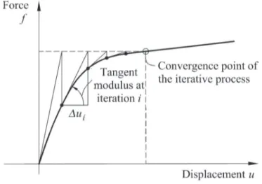
Figure 6 shows the solution for a nonlinear structural system of a single degree of freedom based on the Newton-Raphson process. The arc-length process is a variant of the Newton-Raphson method that controls the progress of the iterative process (Figure 7). The arc-length and load factor are denoted as l and λ, respectively. The incremental process is capable of passing through critical points.

The section analysis and reinforcement design methods are appli-cable, but not limited, to the Sargin stress-strain relationship.

5.1 Arc-length method

The arc-length method presented by Crisfield [14] is an alternative formulation of the method originally proposed by Riks [15]. The stress resultant vector is defined as , where is a load factor and is the stress resultant vector that is established as a reference.

The term ΔSi is defined as:

(36)

where S_i = [N_x,i M_y,i M_z,i] is the stress resultant vector associated with the generalized strain vector k_i = [k_x,i k_y,i k_z,i]T_{at iteration i.} Equation is rewritten as:

(37)

where E_i is a tangent matrix and Dk_i is the increment of the general-ized strain vector at iteration i. Equations (36) and (37) yield:

(38)

where

(39)

(40)

The arc-length l is expressed by:

(41)

The substitution of (38) into (41) yields:

(42)

Expression (42) defines the quadratic equation:

(43)

where

(44)

One of the roots of equation (43) corresponds to the factor λ of the next iteration. The appropriate root is discussed in the next item.

5.2 Section analysis

The parameters required for section analysis are the steel and concrete properties, the geometric characteristics of the cross-sec-tion, the position and area of the reinforcing steel bars, the refer-ence stress resultant vector , and the arc-length l. The maximum load factor found throughout the incremental process defines the cross-section strength.

A brief summary of the iterative process is presented next.

I. Generalized strains k_i at iteration i

Iteration i starts with vector k_i. The first iteration can start with k₁=0.

Figure 6

Newton-Raphson method

Figure 7

(6)

II. Generalized stresses S_i and tangent matrix E_i

The strains ε = pT_k

i, stresses σ(ε), and tangent moduli of elasticity E(ε) are determined for each area element of the steel and con-crete. Expressions (32) and (35) yield the generalized stresses S_i and tangent matrices E_i, respectively.

III. Load factors λ_A and λ_B

Equations (39) and (40) yield the auxiliary vectors and , re-spectively. Load factors λA and λB are the solutions of the quadratic equation established by (43) and (44).

IV. Load factor λ

The root of (43) that pushes forward the incremental process is selected. The first iteration elects λ1 = max (λA, λB). For iteration i>1, equation (38) yields:

(45)

(46)

where ΔkA and ΔkB are the strain vector increments of roots λA and λ_B, respectively.

The slopes θ_A and θ_B of roots λ_A and λ_B are respectively defined as:

(47)

(48)

The load factor λ associated with the maximum slope θ = max (θA, θB) is selected. The corresponding increment ΔkA or ΔkB is denoted as Δki. The generalized strain vector ki+1 of the next iteration is:

(49)

The procedure returns to step II to start a new iteration. The pro-cess terminates when steel or concrete strains reach their limit val-ues. Section strength is defined by , where is the maximum load factor found throughout the incremental process.

5.3 Reinforcement design

The parameters required for reinforcement design are the steel and concrete properties, the geometric characteristics of the cross-section, the position and relative area of each reinforcing steel bar, the minimum and maximum steel ratios, the reference stress resul-tant vector S̅, and the arc-length l. The design stress resultants are defined by λd S̅, where λd is the corresponding load factor. A brief summary of the iterative process is presented next.

I. Stress analysis for minimum reinforcement

The procedure in item 5.2 yields the maximum load factor for the minimum reinforcement A_{s min}. If , the required reinforcement is A_{s min} and the process is terminated. Otherwise,

and A_{s INF} = A_{s min}.

II. Stress analysis for maximum reinforcement

The procedure in item 5.2 yields the maximum load factor

λ

A maxs for the maximum reinforcement

A

s max. If

λ

d

>

λ

As max, the cross-section is not adequate and the process is terminated. Otherwise,

λ

SUP

=

λ

As max and s SUP

=

s max

A

_.

III. Iterative process

The required reinforcement is estimated by linear interpolation

(50)

The procedure in item 5.2 yields the maximum load factor for A_s. If , the new limit is defined by and A_{s SUP} = A_s. Otherwise, and A_{S INF} = A_s.

A new iteration restarts when A_{s SUP} - A_{s INF} >TOL_d, where TOL_d is the tolerance for the reinforcement design. The iterative process ends when A_{s SUP} - A_{s INF} ≤ TOL_d. The required reinforcement is conserva-tively assumed to be A_{s SUP}. This study considers TOL_d = 1 × 10-7_m².

6. Examples and numerical results

The reinforcement design procedure based on the arc-length method is implemented in two Fortran programs, which use parab-ola-rectangle and Sargin curves, respectively. Programs Fx4 and Fx5 are presented in Kabenjabu [16].

The typical rectangular cross-section is defined by by = 0.25 m and b_z= 0.80 m (Figure 8). The rebar edge distances in y and z direc-tions are d'_y = 0.05 m and d'_z = 0.05 m, respectively.

The concrete section is discretized in 25×80 area elements. The section is considered doubly reinforced in most examples, but it is also studied as singly reinforced for pure bending.

The characteristic yield strength of steel is f_yk = 500MPa.

Figure 8

(7)

The examples investigate concrete grades C15, C30, and C45. The corresponding compressive strengths are 15 MPa, 30 MPa and 45MPa, respectively. Although C15 concrete is no longer in use, it is included in the study because of its widespread use in the past.

The partial safety factors for concrete and steel are γ_c= 1.4 and γ_s= 1.15, respectively, as recommended in ABNT NBR 6118:2014 [10]. N_x, M_y, and M_z are the design values of the stress resultants. The examples are summarized in Tables 1 to 9, where A_{s tot} is the required total reinforcement, ε_{c min} is the minimum concrete strain,

and ε_{s max} is the maximum steel strain. The relative difference ΔAs tot ⁄ As tot is defined as:

(51)

where A_{s tot,PAR-RECT} and A_{s tot,SARGIN} are the required total reinforce-ment for parabola-rectangle and Sargin curves, respectively. The section is subjected to pure compression in Table 1. The Sargin curve yields lower reinforcement values than the parabola-rectan-gle diagram. The limit strain ε_cu2 = -0.002 of the parabola-rectangle

Table 1

Doubly-reinforced cross-section subjected to pure compression

Stress resultants Parabola-rectangle diagram Sargin curve Diff. Relative difference N_x

(kN)

M_y (kNm)

M_z (kNm)

A_{s tot}

(cm²) εc min εs max

A_{s tot}

DA_{s tot}

(cm²) DAstot/Astot

C15

-3000 0 0 28.0 -0.00200 -0.00200 27.2 -0.00207 -0.00207 -0.8 -2.9% -4000 0 0 51.8 -0.00200 -0.00200 50.2 -0.00207 -0.00207 -1.6 -3.1% -5000 0 0 75.6 -0.00200 -0.00200 73.2 -0.00207 -0.00207 -2.4 -3.2%

C30

-4000 0 0 8.5 -0.00200 -0.00200 8.2 -0.00216 -0.00216 -0.3 -3.4% -4500 0 0 20.4 -0.00200 -0.00200 19.7 -0.00216 -0.00216 -0.7 -3.4% -5000 0 0 32.3 -0.00200 -0.00200 31.2 -0.00216 -0.00216 -1.1 -3.4% -5500 0 0 44.2 -0.00200 -0.00200 42.7 -0.00216 -0.00216 -1.5 -3.4% -6000 0 0 56.1 -0.00200 -0.00200 54.2 -0.00216 -0.00216 -1.9 -3.4% -6500 0 0 68.0 -0.00200 -0.00200 65.7 -0.00216 -0.00216 -2.3 -3.4% -7000 0 0 79.9 -0.00200 -0.00200 77.2 -0.00216 -0.00216 -2.7 -3.4%

C45

-6000 0 0 12.7 -0.00200 -0.00200 12.3 -0.00240 -0.00240 -0.4 -3.3% -7000 0 0 36.5 -0.00200 -0.00200 35.3 -0.00240 -0.00240 -1.2 -3.3% -8000 0 0 60.3 -0.00200 -0.00200 58.3 -0.00240 -0.00240 -2.0 -3.3%

Table 2

Doubly-reinforced cross-section subjected to compression and uniaxial bending (e

_z

= b

_z

⁄ 4)

(kN)

M_y (kNm)

M_z (kNm)

A_{s tot}

DA_{s tot}

(cm²) DAstot/Astot

C15

-1250 0 250 8.3 -0.00350 0.00077 8.4 -0.00295 0.00085 0.1 1.3% -1750 0 350 24.4 -0.00350 0.00027 24.3 -0.00284 0.00034 0.0 0.0% -2250 0 450 41.7 -0.00350 0.00005 41.6 -0.00275 0.00012 -0.1 -0.2% -2750 0 550 59.4 -0.00345 -0.00008 59.2 -0.00270 -0.00001 -0.2 -0.3% -3250 0 650 77.3 -0.00339 -0.00016 77.1 -0.00266 -0.00009 -0.2 -0.3%

C30

-2250 0 450 9.7 -0.00350 0.00103 10.7 -0.00318 0.00100 1.0 10.1%

-2500 0 500 16.6 -0.00350 0.00077 17.7 -0.00318 0.00077 1.1 6.5%

-2750 0 550 24.2 -0.00350 0.00059 25.3 -0.00317 0.00059 1.1 4.6% -3000 0 600 32.1 -0.00350 0.00045 33.2 -0.00315 0.00046 1.1 3.6% -3250 0 650 40.3 -0.00350 0.00035 41.5 -0.00313 0.00036 1.2 2.9% -3500 0 700 48.7 -0.00350 0.00027 49.9 -0.00311 0.00028 1.2 2.4% -3750 0 750 57.2 -0.00350 0.00020 58.4 -0.00309 0.00021 1.2 2.0% -4000 0 800 65.9 -0.00351 0.00014 67.0 -0.00308 0.00015 1.2 1.8%

C45

-3250 0 650 11.4 -0.00350 0.00115 13.5 -0.00338 0.00105 2.1 18.2%

-3500 0 700 17.9 -0.00350 0.00093 20.2 -0.00339 0.00086 2.3 13.0%

-4000 0 800 32.4 -0.00350 0.00064 35.0 -0.00338 0.00059 2.7 8.2%

-4500 0 900 48.2 -0.00350 0.00045 51.0 -0.00336 0.00041 2.8 5.9%

(8)

diagram is smaller in modulus than the design value of the yield strain of the steel (ε_syd = 0.00207). Steel stresses are higher with the Sargin curve since they reach the yield point. The differences between the two models are small and less than 5% in required reinforcement. Tables 2 and 3 consider combined compression and uniaxial bend-ing with eccentricities of e_z = b_z ⁄ 4 and e_z = b_z ⁄ 2, respectively, where e_z = |M_z ⁄ N_x|. In Table 4, the section is subjected to

com-pression and biaxial bending with e_y = b_y ⁄ 4 and e_z = b_z ⁄ 4, where e_y = |M_y ⁄ N_x|. Table 5 discusses compression and biaxial bending with e_y = b_y ⁄ 2 and e_z = b_z ⁄ 2. Tables 6 and 7 consider compression and uniaxial bending with e_y = b_y ⁄ 4 and e_y = b_y ⁄ 2, respectively. Ta-ble 8 investigates pure bending with compression reinforcement. The relative differences are always less than 5% in Tables 3, 5, 7 and 8.

Table 3

Doubly-reinforced cross-section subjected to compression and uniaxial bending (e

_z

= b

_z

⁄ 2)

(kN)

M_y (kNm)

M_z (kNm)

A_{s tot}

DA_{s tot}

(cm²) DAstot/Astot

C15

-750 0 300 8.3 -0.00350 0.00301 8.4 -0.00259 0.00244 0.1 0.7% -1000 0 400 16.1 -0.00350 0.00170 15.9 -0.00350 0.00188 -0.3 -1.6% -1250 0 500 26.7 -0.00351 0.00126 26.5 -0.00350 0.00140 -0.3 -1.0% -1500 0 600 38.0 -0.00350 0.00101 37.8 -0.00344 0.00112 -0.3 -0.7% -1750 0 700 49.7 -0.00350 0.00085 49.5 -0.00336 0.00094 -0.2 -0.5% -2000 0 800 61.6 -0.00350 0.00075 61.3 -0.00329 0.00081 -0.2 -0.4%

C30

-1000 0 400 7.4 -0.00350 0.00634 7.6 -0.00287 0.00515 0.1 1.9% -1250 0 500 11.6 -0.00350 0.00434 11.8 -0.00290 0.00355 0.2 1.9% -1500 0 600 16.7 -0.00350 0.00301 17.0 -0.00291 0.00248 0.3 1.9% -1750 0 700 22.7 -0.00350 0.00207 23.3 -0.00337 0.00207 0.6 2.7% -2000 0 800 32.2 -0.00350 0.00170 32.8 -0.00350 0.00175 0.5 1.7% -2250 0 900 42.6 -0.00350 0.00144 43.2 -0.00350 0.00149 0.6 1.5% -2500 0 1000 53.4 -0.00351 0.00126 54.1 -0.00351 0.00130 0.7 1.3% -2750 0 1100 64.6 -0.00350 0.00112 65.4 -0.00350 0.00116 0.7 1.1%

C45

-1500 0 600 11.1 -0.00350 0.00634 11.4 -0.00312 0.00532 0.3 2.8% -2000 0 800 19.8 -0.00350 0.00384 20.3 -0.00312 0.00317 0.6 2.8% -2500 0 1000 30.9 -0.00350 0.00235 31.8 -0.00331 0.00207 0.9 2.9% -3000 0 1200 48.4 -0.00350 0.00170 50.3 -0.00350 0.00166 1.9 4.0% -3500 0 1400 69.2 -0.00350 0.00137 71.4 -0.00351 0.00135 2.2 3.2%

Table 4

Doubly-reinforced cross-section subjected to compression and biaxial bending (e

_y

= b

_y

⁄4 and e

_z

= b

_z

⁄4)

(kN)

M_y (kNm)

M_z (kNm)

A_{s tot}

DA_{s tot}

(cm²) DAstot/Astot

C15

-850 53.125 170 9.3 -0.00350 0.00185 8.4 -0.00332 0.00207 -0.8 -9.0%

-1000 62.500 200 15.2 -0.00350 0.00158 13.9 -0.00350 0.00186 -1.3 -8.6%

-1250 78.125 250 26.4 -0.00350 0.00131 25.0 -0.00350 0.00152 -1.4 -5.4%

-1500 93.750 300 38.3 -0.00350 0.00115 36.8 -0.00350 0.00131 -1.4 -3.7% -1750 109.375 350 50.5 -0.00350 0.00105 49.1 -0.00350 0.00118 -1.4 -2.7% -2000 125.000 400 62.8 -0.00350 0.00098 61.5 -0.00350 0.00109 -1.3 -2.1% -2250 140.625 450 75.3 -0.00350 0.00092 74.0 -0.00350 0.00102 -1.3 -1.7%

C30

-1500 93.750 300 11.8 -0.00350 0.00211 11.8 -0.00350 0.00229 0.0 0.2% -1750 109.375 350 20.4 -0.00350 0.00180 19.8 -0.00350 0.00193 -0.6 -3.0% -2000 125.000 400 30.5 -0.00350 0.00158 29.8 -0.00350 0.00170 -0.7 -2.4% -2250 140.625 450 41.4 -0.00350 0.00143 40.6 -0.00350 0.00152 -0.7 -1.8% -2500 156.250 500 52.8 -0.00350 0.00131 52.1 -0.00350 0.00140 -0.7 -1.4% -2750 171.875 550 64.5 -0.00350 0.00122 63.8 -0.00350 0.00130 -0.7 -1.1%

C45

-2000 125.000 400 11.1 -0.00350 0.00243 11.9 -0.00350 0.00242 0.8 7.3%

-2250 140.625 450 17.6 -0.00350 0.00211 18.6 -0.00350 0.00210 1.0 5.4%

(9)

Table 5

Doubly-reinforced cross-section subjected to compression and biaxial bending (e

_y

= b

_y

⁄2 and e

_z

= b

_z

⁄2)

Table 6

Doubly-reinforced cross-section subjected to compression and uniaxial bending (e

_y

= b

_y

⁄4)

(kN)

M_y (kNm)

M_z (kNm)

A_{s tot}

DA_{s tot}

(cm²) DAstot/Astot

C15

-400 50 160 10.3 -0.00350 0.00364 9.8 -0.00350 0.00407 -0.5 -4.8% -600 75 240 21.2 -0.00350 0.00268 20.6 -0.00350 0.00300 -0.6 -2.7% -800 100 320 33.2 -0.00350 0.00216 32.7 -0.00337 0.00232 -0.5 -1.5% -1000 125 400 47.6 -0.00350 0.00191 45.6 -0.00350 0.00205 -2.0 -4.3% -1200 150 480 63.1 -0.00350 0.00177 61.0 -0.00350 0.00189 -2.1 -3.3%

C30

-600 75 240 11.7 -0.00350 0.00456 11.4 -0.00350 0.00477 -0.2 -2.0% -800 100 320 20.7 -0.00350 0.00364 20.4 -0.00350 0.00381 -0.3 -1.4% -1000 125 400 31.0 -0.00350 0.00308 30.8 -0.00350 0.00323 -0.3 -0.9% -1200 150 480 42.3 -0.00350 0.00268 42.0 -0.00350 0.00281 -0.3 -0.6% -1400 175 560 54.1 -0.00350 0.00239 53.9 -0.00350 0.00251 -0.2 -0.4% -1600 200 640 66.3 -0.00350 0.00216 66.2 -0.00350 0.00226 -0.1 -0.2%

C45

-600 75 240 7.5 -0.00350 0.00634 7.6 -0.00350 0.00630 0.1 1.8% -800 100 320 13.6 -0.00350 0.00500 13.9 -0.00350 0.00498 0.3 1.9% -1000 125 400 21.7 -0.00350 0.00419 22.1 -0.00350 0.00417 0.4 1.8% -1200 150 480 31.0 -0.00350 0.00364 31.5 -0.00350 0.00363 0.5 1.6% -1400 175 560 41.2 -0.00350 0.00324 41.8 -0.00350 0.00323 0.6 1.4% -1600 200 640 52.1 -0.00350 0.00293 52.8 -0.00350 0.00292 0.7 1.3% -1800 225 720 63.5 -0.00350 0.00268 64.2 -0.00350 0.00267 0.8 1.2%

(kN)

M_y (kNm)

M_z (kNm)

A_{s tot}

DA_{s tot}

(cm²) DAstot/Astot

C15

-1250 78.125 0 12.2 -0.00350 0.00048 12.3 -0.00286 0.00056 0.1 1.2% -1500 93.750 0 22.0 -0.00350 0.00031 22.1 -0.00280 0.00037 0.1 0.3% -1750 109.375 0 32.2 -0.00350 0.00021 32.2 -0.00277 0.00027 0.0 0.0% -2000 125.000 0 42.5 -0.00350 0.00014 42.4 -0.00275 0.00020 -0.1 -0.1% -2250 140.625 0 52.8 -0.00350 0.00010 52.8 -0.00274 0.00015 -0.1 -0.1% -2500 156.250 0 63.3 -0.00350 0.00006 63.2 -0.00273 0.00011 -0.1 -0.2% -2750 171.875 0 73.7 -0.00350 0.00004 73.6 -0.00272 0.00008 -0.1 -0.2%

C30

-2100 131.250 0 9.7 -0.00350 0.00075 11.0 -0.00304 0.00071 1.3 13.9%

-2250 140.625 0 15.0 -0.00350 0.00063 16.4 -0.00307 0.00061 1.4 9.3%

-2500 156.250 0 24.3 -0.00350 0.00048 25.7 -0.00308 0.00048 1.4 5.9%

-2750 171.875 0 34.1 -0.00350 0.00038 35.5 -0.00308 0.00039 1.4 4.2% -3000 187.500 0 44.0 -0.00350 0.00031 45.5 -0.00307 0.00032 1.4 3.3% -3250 203.125 0 54.1 -0.00350 0.00025 55.5 -0.00307 0.00026 1.4 2.6% -3500 218.750 0 64.3 -0.00350 0.00021 65.8 -0.00306 0.00022 1.4 2.2% -3750 234.375 0 74.6 -0.00350 0.00017 76.0 -0.00306 0.00019 1.4 1.9%

C45

-3000 187.500 0 9.6 -0.00350 0.00086 12.4 -0.00323 0.00074 2.8 28.7%

-3250 203.125 0 18.0 -0.00350 0.00069 21.1 -0.00327 0.00061 3.1 17.0%

-3500 218.750 0 27.1 -0.00350 0.00057 30.3 -0.00328 0.00051 3.2 11.9%

-3750 234.375 0 36.5 -0.00350 0.00048 39.8 -0.00329 0.00044 3.4 9.2%

-4000 250.000 0 46.2 -0.00350 0.00041 49.6 -0.00329 0.00038 3.4 7.4%

-4250 265.625 0 56.0 -0.00350 0.00036 59.5 -0.00329 0.00032 3.5 6.2%

-4500 281.250 0 66.0 -0.00350 0.00031 69.6 -0.00329 0.00028 3.5 5.3%

(10)

Table 8

Doubly-reinforced cross-section subjected to pure bending

(kN)

M_y (kNm)

M_z (kNm)

A_{s tot}

DA_{s tot}

(cm²) DAstot/Astot

C15

0 0 150 9.7 -0.00147 0.01000 9.7 -0.00130 0.01001 0.0 -0.1% 0 0 300 19.7 -0.00189 0.01000 19.7 -0.00177 0.01000 0.0 0.2% 0 0 450 29.6 -0.00211 0.01001 29.7 -0.00202 0.01001 0.1 0.2% 0 0 600 39.5 -0.00225 0.01001 39.6 -0.00218 0.01000 0.1 0.2% 0 0 750 49.4 -0.00235 0.01000 49.5 -0.00229 0.01000 0.1 0.2% 0 0 900 59.3 -0.00242 0.01000 59.4 -0.00237 0.01001 0.1 0.2% 0 0 1050 69.2 -0.00247 0.01001 69.3 -0.00242 0.01001 0.1 0.2%

C30

0 0 150 9.6 -0.00109 0.01000 9.6 -0.00100 0.01000 0.0 -0.2% 0 0 300 19.5 -0.00147 0.01000 19.5 -0.00140 0.01000 0.0 0.0% 0 0 450 29.4 -0.00172 0.01000 29.4 -0.00166 0.01001 0.0 0.1% 0 0 600 39.3 -0.00189 0.01000 39.4 -0.00184 0.01001 0.0 0.1% 0 0 750 49.3 -0.00202 0.01000 49.3 -0.00197 0.01000 0.1 0.1% 0 0 900 59.2 -0.00211 0.01001 59.2 -0.00208 0.01000 0.1 0.1% 0 0 1050 69.1 -0.00219 0.01000 69.2 -0.00216 0.01001 0.1 0.1%

C45

0 0 150 9.5 -0.00090 0.01000 9.5 -0.00088 0.01000 0.0 0.0% 0 0 300 19.3 -0.00124 0.01001 19.3 -0.00123 0.01001 0.0 0.1% 0 0 450 29.2 -0.00147 0.01000 29.2 -0.00147 0.01001 0.0 0.1% 0 0 600 39.1 -0.00165 0.01000 39.2 -0.00165 0.01000 0.0 0.1% 0 0 750 49.1 -0.00178 0.01000 49.1 -0.00178 0.01000 0.0 0.1% 0 0 900 59.0 -0.00189 0.01000 59.0 -0.00189 0.01001 0.0 0.1% 0 0 1050 68.9 -0.00198 0.01000 69.0 -0.00198 0.01001 0.0 0.1%

Table 7

Doubly-reinforced cross-section subjected to compression and uniaxial bending (e

_y

= b

_y

⁄2)

(kN)

M_y (kNm)

M_z (kNm)

A_{s tot}

DA_{s tot}

(cm²) DAstot/Astot

C15

-750 93.75 0 12.1 -0.00350 0.00214 12.6 -0.00344 0.00248 0.4 3.4% -1000 125.00 0 24.9 -0.00350 0.00148 24.7 -0.00350 0.00161 -0.2 -0.9% -1250 156.25 0 39.1 -0.00350 0.00120 38.9 -0.00350 0.00129 -0.2 -0.6% -1500 187.50 0 53.8 -0.00350 0.00105 53.6 -0.00339 0.00111 -0.2 -0.5% -1750 218.75 0 68.7 -0.00350 0.00095 68.5 -0.00344 0.00101 -0.2 -0.3%

C30

-1000 125.00 0 11.2 -0.00350 0.00471 11.7 -0.00307 0.00399 0.5 4.4% -1250 156.25 0 17.1 -0.00350 0.00321 17.9 -0.00350 0.00327 0.8 4.5% -1500 187.50 0 24.3 -0.00350 0.00214 25.0 -0.00332 0.00207 0.7 3.1% -1750 218.75 0 36.4 -0.00350 0.00172 37.3 -0.00350 0.00175 0.9 2.4% -2000 250.00 0 49.8 -0.00350 0.00148 50.7 -0.00350 0.00151 0.9 1.8% -2250 281.25 0 63.9 -0.00350 0.00132 64.8 -0.00350 0.00135 1.0 1.5% -2500 312.50 0 78.2 -0.00350 0.00120 79.2 -0.00350 0.00123 1.0 1.3%

C45

(11)

The examples in Tables 2, 4, and 6, which consider combined compression and bending with smaller eccentricity, yield significant relative differences. A relative difference of -9.0% is found for C15 concrete (Table 4). The negative sign means that the

parabola-rectangle diagram is more conservative. C30 and C45 concretes yield relative differences of 13.9% and 28.7%, respectively (Table 6). The positive sign means that the Sargin curve requires more reinforcement. As the absolute differences for C15, C30 and C45 are limited to -1.4 cm2_{, 1.4 cm}2_{, and 3.6 cm}2_{, respectively, the} rela-tive differences are relevant for low reinforcement ratios.

Table 9 investigates reinforcement design in pure bending with-out compression reinforcement. The concrete class is C30. This analysis demonstrates the good convergence of the proposed method even without any contribution from steel to the stiffness of the compressive block. The relative differences are less than 1% in the first examples, when the tension reinforcement reaches the yield point (εsmax ≥ 0.00207). In the last example, the relative differ-ence is 5.7% and the reinforcement strain is below the yield point. ABNT NBR 6118:2014 [10] recommends compression reinforce-ment in beams to avoid a neutral axis in domain 4. The comparison between the same examples with and without compression rein-forcement (Tables 8 and 9) shows that this recommendation also improves the correspondence between the parabola-rectangle and Sargin results in pure bending.

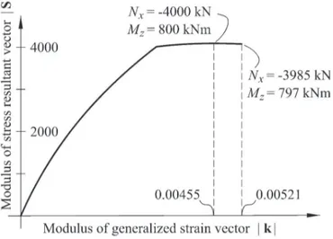
Figure 9 examines an example for the Sargin curve in Table 2 (e_z = b_z ⁄ 4, f_ck= 30MPa, and A_{s total} = 67.0 cm2_{). The modulus of the} stress resultant vector |S| is plotted as a function of the modulus of the generalized strain vector |k|. The maximum strength value is obtained for |k|=0.00455, which corresponds to ε_{c min} = -0.00308,

Table 9

Singly-reinforced cross-section subjected to pure bending

(kN)

M_y (kNm)

M_z (kNm)

A_{s tot}

DA_{s tot}

(cm²) DAstot/Astot

C30

0 0 150 4.8 -0.00126 0.01001 4.8 -0.00113 0.01000 0.0 -0.2% 0 0 300 9.9 -0.00212 0.01000 9.9 -0.00199 0.01000 0.0 0.0% 0 0 450 15.3 -0.00317 0.01000 15.4 -0.00286 0.00920 0.0 0.2% 0 0 600 21.4 -0.00350 0.00710 21.5 -0.00286 0.00568 0.1 0.4% 0 0 750 28.2 -0.00350 0.00449 28.4 -0.00291 0.00366 0.2 0.6% 0 0 900 36.1 -0.00350 0.00271 36.4 -0.00281 0.00207 0.3 0.8% 0 0 1050 70.5 -0.00350 0.00135 74.6 -0.00350 0.00131 4.0 5.7%

Figure 9

Section under compression and uniaxial bending

(e

_z

= b

_z

⁄4, f

_ck

= 30 MPa and A

_{s tot}

= 67.0 cm

2

₎

Figure 10

(12)

N_x = -4000 kN, and M_z = 800 kNm. However, ultimate concrete strain is reached for |k|=0.00521, which corresponds to εc min = -0.0035, N_x = -3985 kN, and M_z = 797 kNm.

Figure 10 investigates an example in pure flexion without com-pression reinforcement (Table 9, M_z = 1050 kNm). The resul-tants of the compressive stresses in concrete are obtained by numerically integrating the parabola-rectangle and Sargin curves. The required reinforcements are A_{s PAR-RECT} = 70.54 cm² and A_{s SARGIN} = 74.56 cm², respectively. The corresponding level arms are z_{s PAR-RECT} = 0.524 m and z_{s SARGIN} = 0.510 m, respectively. Reinforc-ing bars do not reach the yield point in either case. The parabola-rectangle diagram and the Sargin curve yield σc topo = σc min and |σc top| < |σc min|, respectively, where σc top is the stress at the top of the section and σc min is the minimum compressive stress in the concrete. The concrete and steel force resultants are R_c = R_s= 2003.73 kN and R_c = R_s = 2057.53 kN for the parabola-rectangle and Sargin curves, respectively.

7. Conclusion

The reinforcement design of concrete sections based on the parabo-la-rectangle diagram is a practical and well-established model. How-ever, the initial modulus of elasticity and plastic range of the parabola-rectangle diagram do not represent the actual behavior of concrete. Stress-strain relationships that better characterize concrete prop-erties are needed for global limit analyses of concrete structures that consider their physical and geometric non-linear behavior. The Sargin curve is selected because it is a function of the peak point and initial modulus of elasticity and represents the descending branch of the stress-strain relationship.

This research proposes a numerical procedure for the reinforce-ment design of concrete sections that uses an arc-length method and yields good convergence in the descending branch of the Sar-gin curve, without having to consider the distributions of strain lim-its around pivot C in domain 5. Strain limlim-its for concrete and steel are not required, but they are included in order to avoid exces-sive deformation. The parabola-rectangle and Sargin curves are considered by using the code provisions for cross-sections and global limit analyses, respectively. The reinforcement design using the parabola-rectangle diagram is based on the section model in ABNT NBR 6118: 2014 [10]. The Sargin curve is implemented ac-cording to the global nonlinear model in CEN Eurocode 2: 2004 [8]. The examples consider characteristic concrete strength values of 15, 30, and 45 MPa. The typical 0.25 m × 0.85 m rectangular cross-section is subjected to several loading cases which include pure compression and pure bending. Eccentricities in each direc-tion of 1/4 and 1/2 of the corresponding dimension are considered in uniaxial and biaxial bending.

The required reinforcement shows a good correspondence in pure compression, pure bending of doubly-reinforced cross-sections, and uniaxial and biaxial bending with the highest relative eccen-tricity. The results also show good correspondence in pure bending of singly-reinforced cross-sections when reinforcing steel reaches the yield point. The comparison of the results shows that the use of compression reinforcement in beams to avoid the neutral axis in domain 4 also improves the correspondence between the results of the parabola-rectangle and Sargin curves.

More significant differences are observed in uniaxial and biaxial bending with the lowest relative eccentricity. The parabola-rectan-gle diagram is more conservative for C15 concrete, which shows a relative difference of -9.0%. The Sargin curve yields more rein-forcement for C30 and C45, which present relative differences of 13.9% and 28.7%, respectively. The relative differences are higher for the lower reinforcement ratios, since the absolute differences are small and limited to -1.4 cm2_{, 1.4 cm}2_{, and 3.6 cm}2_{for C15,} C30, and C45, respectively.

Despite the good correspondence observed in most examples, the investigation shows that the results of the Sargin curve are not necessarily conservative when compared to the parabola-rect-angle diagram. For this reason, a global limit analysis using the Sargin curve still requires the analysis of all cross-sections with the parabola-rectangle diagram.

The proposed reinforcement design method is efficient, numerically robust, and capable of considering other stress-strain relationships with or without descending branches. The examples use local and global analysis parameters for the parabola-rectangle and Sargin curves, respectively. The validation of a single calculation model for section and global limit analyses could motivate future investigations.

8. Acknowledgements

The first author thanks the Coordination for the Improvement of Higher Education Personnel (CAPES) for financial support. The au-thors thank the valuable suggestions of Prof. Benjamin Ernani Diaz.

9. References

[1] MÖRSCH, E. Concrete-steel construction (Der Eisenbet-onbau), The Engineering News Publishing Company, New York, 1910, 368 p.

[2] HOGNESTAD, E. A study of combined bending and axial load in reinforced concrete members, Bulletin Series no. 399, Engineering Experiment Station, University of Illinois, Urbana, 1951, 128 p.

[3] WHITNEY, C. S. Design of reinforced concrete members un-der flexure or combined flexure and direct compression, ACI Journal, v. 33, n. 1, 1937, p. 483-498.

[4] BITTNER, E. Zur Klärung der n-Frage bei Eisenbetonbalken, Beton und Eisen, 1935, v. 34, n.14, p. 226-228.

[5] MATTOCK, A. H., KRIZ, L. B., AND HOGNESTAD, E. Rect-angular concrete stress distribution in ultimate strength de-sign, ACI Journal, 1961, v. 57, n. 2, p. 875-928.

[6] RÜSCH, H., GRASSER, E., AND RAO, P. S. Principes de calcul du béton armé sous états de contraintes monoaxiaux, Bulletin d’Information n. 36, CEB, Paris, 1962, p. 1-112. [7] AMERICAN CONCRETE INSTITUTE. Building code

re-quirements for structural concrete - ACI 318-14, Farmington Hills, 2015.

[8] COMITÉ EUROPÉEN DE NORMALISATION. Eurocode 2: Design of concrete structures – Part 1-1: General rules and rules for buildings - EN 1992-1-1, Brussels, 2004.

(13)

[10] ASSOCIAÇÃO BRASILEIRA DE NORMAS TÉCNICAS. Projeto de estruturas de concreto –Procedimento – ABNT NBR 6118, Rio de Janeiro, 2014.

[11] SARGIN, M. Stress-strain relationships for concrete and the analysis of structural concrete sections, SM Study n. 4, Solid Mechanics Division, University of Waterloo, Waterloo, Cana-da, 1971, 167 p.

[12] COMITÉ EURO-INTERNATIONAL DU BÉTON, FÉDÉRA-TION INTERNAFÉDÉRA-TIONALE DE LA PRÉCONTRAINTE. CEB-FIP Model Code 1990, Thomas Telford, London, 1993, 437 p. [13] RÜSCH, H. Researches toward a general flexural theory of

structural concrete. ACI Journal, v. 57, n. 7, 1960, p. 1-28. [14] CRISFIELD, M. A. A fast incremental/iterative solution

proce-dure that handles “snap-through”, Computers & Structures, 1981, v. 13, n. 1-3, p. 55-62.

[15] RIKS, E. An incremental approach to the solution of snap-ping and buckling problems, International Journal of Solids Structures, 1979, v. 15, n. 7, p. 529-551.